1. Introduction
Irrigation is increasingly becoming crucial in sustainable food production worldwide. While only 20% of the total cultivated area is irrigated, it accounts for 40% of the agricultural production [
1,
2]. Irrigation is not equally distributed either over the globe or within the most active agricultural areas. In fact, there are some regions where irrigation is more widely employed (e.g., India) than others (Sahel region) [
3]. The reason for its development and use in most cases is a combination between climate conditions and food demand [
1]. Considering environmental factors, a changing climate might pose a threat. In fact, most of the productive agricultural areas are situated in regions defined as vulnerable to negative impacts due to climate change [
4,
5,
6]. Climate change impacts on agriculture are commonly related to heat waves and drought conditions, which are projected to increase in both intensity and frequency for these areas [
6]. Therefore, those agricultural regions that rely on irrigation to sustain food production could be strongly affected.
However, irrigation is not only affected by the climate, irrigation modifies the climate as well. In fact, irrigation has a cooling effect on the surface temperature, e.g., [
7,
8,
9]. By moistening the ground, more of the incoming energy is partitioned into the latent heat, reducing the sensible heat, which is linked to the surface temperature [
10,
11,
12,
13,
14]. Such changes reflect the local conditions as both the moisture content and the vertical temperature profile are affected [
15,
16,
17]. Changes in the vertical profile might affect the air mass thermodynamical properties as well as the vertical structure within the boundary layer [
15,
18,
19]. As irrigation is not spatially uniform, a discontinuity in the horizontal surface fluxes causes local circulation changes [
7,
20,
21,
22]. In some regions, irrigation is found to affect the precipitation either locally or in the downwind area, due to atmospheric water vapor transport [
23,
24,
25]. However, the effect varies depending on the geographical location, the general climate conditions, the model scales, and the representation of irrigation.
Global studies have found that the magnitude of temperature cooling and other local responses differ depending on the geographical region [
9,
15,
26,
27], as the land-atmosphere coupling [
9,
28] as well as the synoptic conditions [
12,
14,
16,
29] might mask the soil moisture response to irrigation. These studies identified key regions, both for the importance held by irrigation within the social-economic structure, as well as its impact on the atmosphere and climate. The Asian continent, the United States, and the Mediterranean area show different impacts of irrigation. Several studies address the local impacts with higher resolution models, which are able to better capture the influence of the smaller scale perturbations, e.g., [
12,
14,
29,
30,
31]. The Mediterranean area has been studied intensively only in Thiery et al. [
9], with a global model, finding that the strong land-atmosphere coupling has irrigation that greatly impacts the local climate. In this region it was previously found that local conditions due to irrigation might trigger parameterized convection [
9,
26], having a primarily convective response. However, limited-area convection-permitting simulations must be performed to properly assess how convection interacts with surface changes.
As far as climate change is concerned, the irrigation context is that of water scarcity and the limiting of its availability under future projections [
32]. Even for past climate change, irrigation has contributed to the masking of the warming signal in highly irrigated regions, such as California [
33,
34]. Also, the irrigation parameterization itself has been found to be a major cause of uncertainties in past studies [
24,
26].
While it might be argued that these are different problems, we must remember that numerical models are created and validated on past climate conditions. Not representing a process within a numerical model causes an intrinsic bias, which in the cases of an operational forecast or reanalyses might be corrected with data assimilation, as the observations already include an irrigation signal [
24]. The only model that has an optional irrigation parameterization is the Community Land Model (CLM4, [
35]). This model is mostly used for global studies when coupled to the atmospheric component (CAM) in its Community Earth System Model (CESM), and it is more suitable for a global statistical approach. CLM4 can be coupled with the limited area Weather Research and Forecasting (WRF) model, to study more specific events and regions [
36], but the parameterization does not resemble the irrigation techniques widely applied across the globe. In fact, irrigation water is determined from the soil wilting point, and applied to the soil layers over a specific amount of time during the day. While this method ensures a closed water budget equation, it does not have irrigation interacting with the canopy or the atmosphere, as might happen for a sprinkler (center-pivot or rain-like) [
3,
37,
38,
39,
40]. Also, most of the used parameterizations do not account for the water applied explicitly [
11,
12,
41,
42], leading to an overestimation of the total amount [
16,
26]. The newly developed parameterization for WRF resembles several irrigation techniques with different evaporative components from the water applied, as well as an explicit treatment of both water used and timing [
43].
The study presented here aims to investigate the effect of irrigation on a highly irrigated area of the Mediterranean region, the Po Valley, with a convection-permitting simulation. The simulation focuses on two consecutive months with different synoptic backgrounds, which are discussed in the first part of
Section 2.1. The simulations are performed using the widely adopted WRF model, with the newly developed parameterizations (
Section 2.2).
3. Results
The results presented here start by discussing the role of the irrigation in the soil moisture balance, relating it to the synoptic conditions. Once two different synoptic periods are identified from the soil moisture time-series, the impact on the surface energy balance is considered for each state. The impact on the whole area is considered as monthly percentage changes with respect to the control, as well as the diurnal cycles. As changes in fluxes affect the near surface temperature, the spatial behavior of the 2-m temperature is discussed, as the irrigation has a nonuniform spatial field.
To provide a more comprehensive view of the irrigation role in modifying the atmospheric state, the correlations of changes of pairs of variables with respect to the control simulations are discussed.
3.1. Soil Moisture
As previously discussed, the synoptic conditions might modulate the irrigation signal as soil moisture is strongly affected by these conditions. In fact, soil moisture temporal changes are influenced by the incoming and outgoing water for each layer. The main input term in this balance equation is the rain, in the absence of irrigation. The water can leave the surface layer mainly through evapotranspiration, surface run-off and ground run-off [
28] (This balance is considered only as a starting point, not for representative of what actually might be observed/simulated). In accounting for soil moisture changes, both precipitation and irrigation play a key role, being external inputs driven mainly by separate components. It might be assumed that, also for this region, the synoptic state for the studied period and region might play a key role. To investigate this assumption, a time-series of the first layer soil moisture is shown in
Figure 2 below.
Given the previously described characteristics of the period chosen, June 2015 is a month with average precipitation, and July 2015 is an exceptional month with almost no precipitation events [
56,
57]. As seen from
Figure 2, May is the spin-up time for soil moisture, with irrigation starting on the 15th. At the start of June, the irrigated runs already have significantly higher values with respect to the control. June soil moisture reflects that the last part of the month is the onset of the July heat wave. Therefore, soil moisture starts to decrease after the last widespread precipitation event of 25 June. While in June, irrigation accounts for 10–30% change in soil moisture, the July values are up to 55%. The reason for dividing June and July is both due to the different magnitude of the irrigation impact and due to the small precipitation event registered in all irrigated runs at the end of June.
As soil moisture affects evaporation, the surface flux partition is studied next.
3.1.1. Surface Fluxes
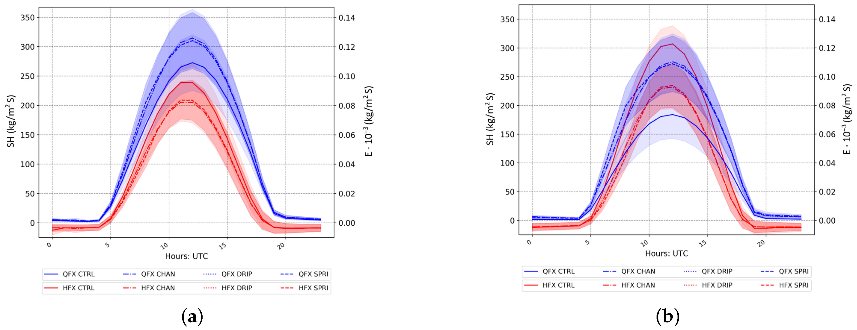
As soil moisture changes impact the surface energy balance partition, a difference between the two months is expected. As the diurnal cycle is strongly modulating the fluxes, for each month it is computed averaging the fields over the irrigated area highlighted in
Figure 1b. The result obtained for the three irrigated simulations as well as the control run are shown in
Figure 3. Firstly, the partition between sensible heat (HFX) and upward moisture flux (QFX) (also Bowen ratio, if the upward moisture flux is converted in latent heat) is very different between the two months. Matching the axes between
and
allows one to compare the two fields without converting the values (as it is scaled by the latent heat of evaporation). In June, the latent heat flux is higher than the sensible flux, which is not true for July. While, in general, the irrigated run behaves similarly, by increasing the upward moisture flux and decreasing the sensible heat flux, the magnitude changes drastically between the two months.
To better understand the magnitude of the changes,
Table 1 summarizes the integrated values and their percentage change with respect to the control for each month and parameterization. Irrigation causes the heat flux to decrease up to
for June and
in July. On the other hand, the moisture fluxes are increased up to
in June and to
in July. Such a drastic increase reflects the extreme conditions of July 2015 and the persistence of the heat wave conditions. In terms of integrated fluxes, irrigation allows to have similar values between the two months, which was not true in the control run. The integrated values do not change greatly, also depending on the parameterization used, the bigger difference is observed between the channel method and the other two. This agrees with the fact that the drop evaporation and drift processes that the sprinkler scheme assumes do not greatly affect the averaged fields. The bigger difference in soil moisture is related to canopy interception and evaporation [
43].
Such an impact on the diurnal cycle reflects on atmospheric quantities, such as the 2-m temperature and moisture content.
3.1.2. Surface Fields
As the irrigation mask does not have a constant spatial distribution, the atmospheric quantities discussed in this part are presented averaged in time, but not in space. This information is complementary to the previously shown time-series, as it helps to relate the spatial variation to the temporal one in assessing the impact of irrigation. To better quantify the differences between the two months, both the differences between the monthly averaged quantities and the absolute values obtained in the control run are shown.
Sensible heat and upward moisture fluxes are expected to strongly influence the near-surface temperature and moisture. As expected from previous studies, the fluxes are impacted more during the middle of the day rather than the nighttime period, e.g., [
7,
12,
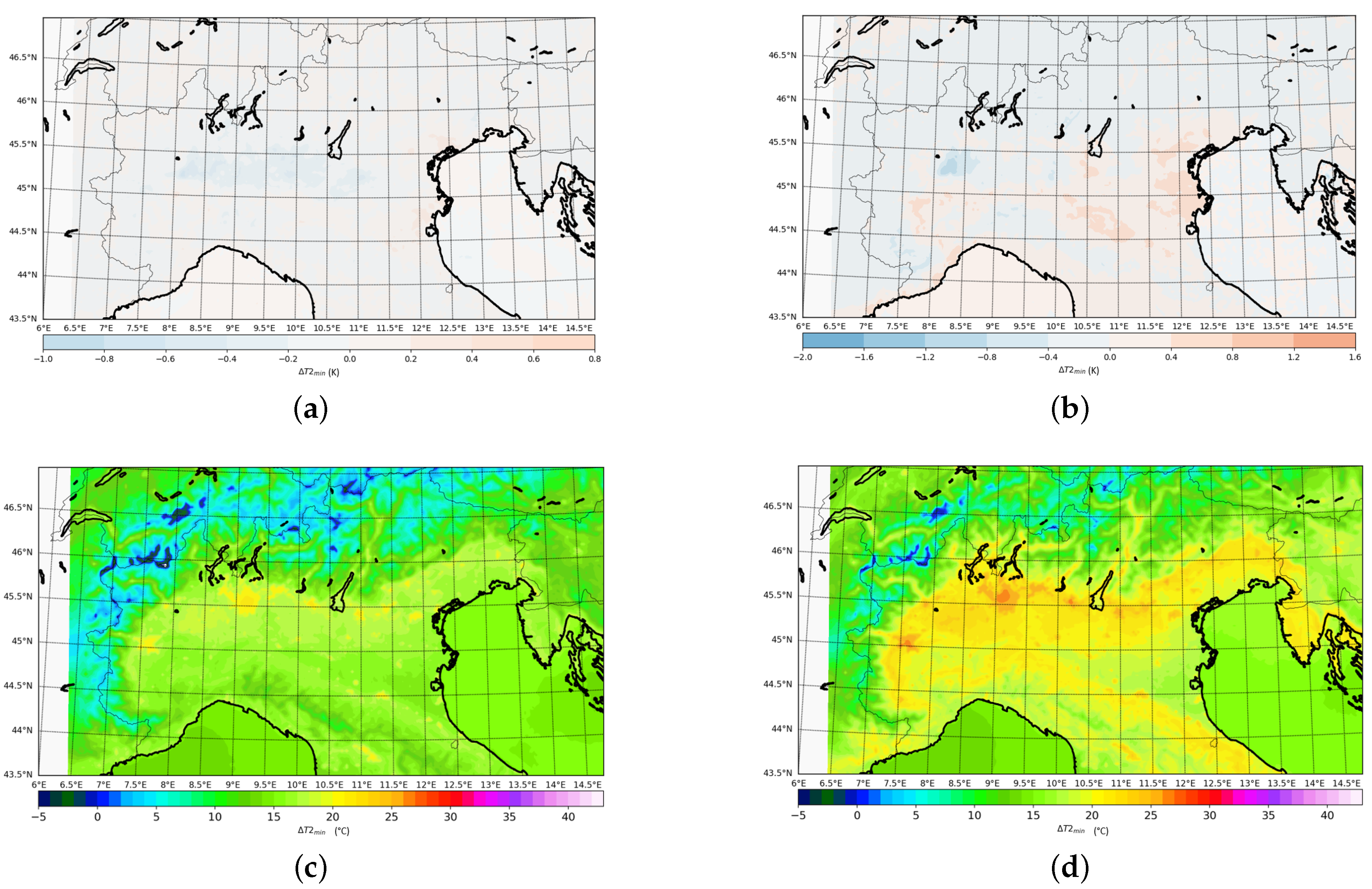
15], as irrigation affects the partition of the incoming energy. This leads to having the maximum T2 as the daily quantity that is more strongly affected. On the other hand, the daily minimum temperature should not be greatly impacted. As the differences in T2 between the irrigated run and the control one obtained for each parameterization are similar to each-other, only the drip case is shown for brevity. The maximum daily 2-m height temperature is investigated in
Figure 4. First, as previously mentioned when the simulation period was introduced, the two months present very different climate conditions. From the monthly average of the maximum T2 obtained in the control simulation, June has an average value of 30
C (
Figure 4c) but July is above 34
C (
Figure 4d). The irrigation impact on the daily T2 maximum is different between the two months, as it affects July more strongly than June. In fact, in July the differences are up to 2.5–3 K cooling, and up to 0.75–1 K for June. Also, the spatial pattern of the difference field seems to agrees with the irrigation map (
Figure 1b) both in location and magnitude, for both months.
The minimum temperature seems not to be affected by irrigation either in June nor in July (
Figure 5a,b), with maximum absolute values of
K. This is expected when considering only the fluxes and their changes, as
Figure 3 showed little-to-no impact in the nighttime. However, it is to be remembered that the effects of changes in the coupled atmosphere-soil components can extend beyond the specific event temporal and spatial scales. As observed before, soil moisture has a longer time scale impact showing a lower decrease in the values observed in all irrigated runs with respect to the control (
Figure 2). However, this reasoning is not limited only to such variables, as changes in the surface might affect the local atmospheric circulation, which can impact the minimum temperatures. In this specific case, no change in the minimum temperature can be related to the lack of irrigation impact on circulation or to a strong soil-atmosphere coupling that modulates all other variations. Some parts of the irrigated Po Valley show an increase in the July minimum temperatures of 0.4–0.8 K (
Figure 5b). However, no spatial correlation with the irrigation map can be found for a possible causality effect.
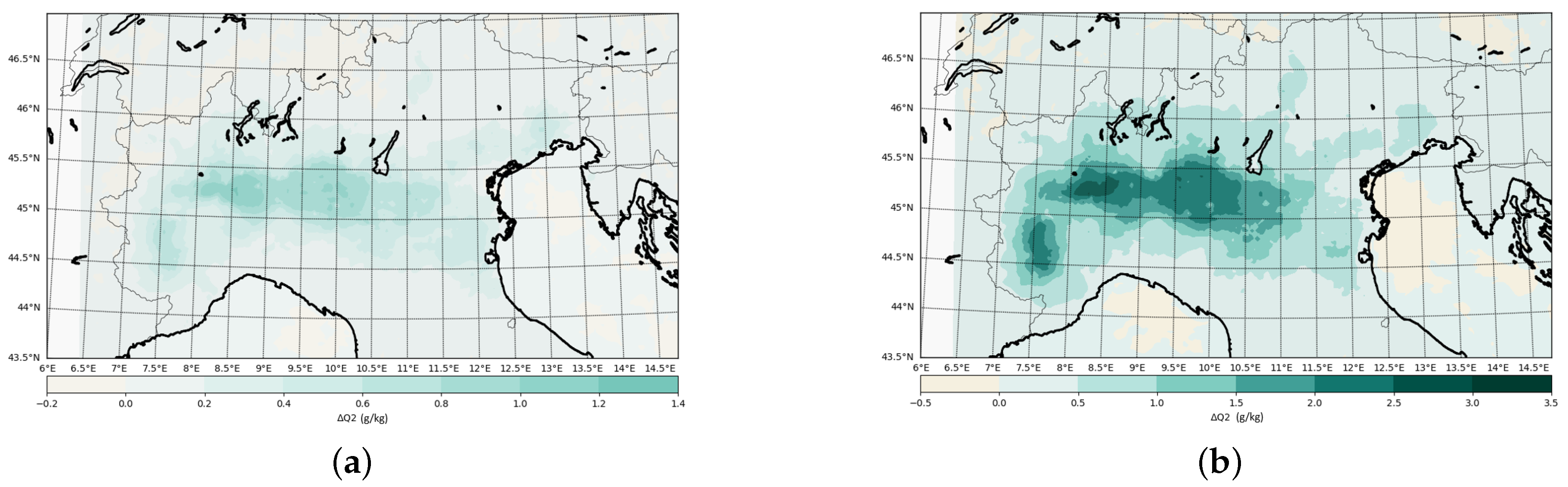
An increase in the upward moisture flux might affect the atmospheric moisture content. Therefore, the 2-m height moisture content (g/kg) is presented in
Figure 6 for the daily monthly average. The daily average is chosen as it is less affected by sub-daily local maxima due to precipitation or convergence events. On average the control mean Q2 does not change much between June and July for the Po Valley region, keeping it close to 7–9 g/kg. Irrigation seems to strongly affect the local values with the expected spatial pattern of the irrigation mask. The daily
T2 maximum, and also the
Q2 changes depending on the month are considered. In fact, in June (
Figure 6a), irrigation causes an increase up to 10%, and in July (
Figure 6b), between 25% and 50%.
Such changes in the lower atmosphere might affect the vertical structure. Therefore, the next part investigates the diurnal cycle of some of the atmospheric variables that might be impacted.
3.2. Diurnal Cycle
Both the potential temperature and the atmospheric moisture content (QV) are affected by the changes at the surface observed in the previous section. Also for this case, all three parameterizations behave similarly, so only one example is shown and discussed. To be consistent, the drip case is chosen, as in the previous sections.
When considering the diurnal cycle calculation of
Figure 7, we acknowledge that it is a result of an averaging process. Therefore, the differences in the fields are significant only if the standard deviation of the spatial differences are smaller compared to them. This is used to ensure that the obtained impact of the irrigation is not a result of the high variability of the boundary layer, but a physical signal. For June
has a standard deviation up to 0.3 K for the lower part of the boundary layer during the middle of the day, and up to 0.24 K for the nighttime. Similarly, the
QV standard deviation accounts for up to 50% of the signal. A lower ratio between the
-fields and their standard deviation is obtained for the month of July.
As expected from the previous results, the vertical structure is also impacted differently in the two months (
Figure 7). The potential temperature differences (
) have an increase up to 50% from June (
Figure 7a) to July (
Figure 7b). However, the changes in
are not uniform in the diurnal cycle nor across the vertical scale. As expected, the maximum impact of irrigation is observed during the middle of the day as the impact of irrigation on the fluxes behaves similarly. As for the impact of irrigation on the minimum temperatures (
Figure 5a,b), from the top panel of
Figure 7 we see that the potential temperature is not affected greatly during the nighttime in both months. The vertical propagation of the irrigation cooling effect depends on the time of the day, but the magnitude and final height is different between June and July. This affects the vertical structure of the boundary layer. In fact, it lowers significantly the height of the boundary layer, causing a later onset of the residual layer for July.
A change in the boundary layer structure affects the vertical profile of the water vapor, as can be observed in the lower panel of
Figure 7. In fact, the vertical distribution is strongly modulated by the changes in the boundary layer. This can be seen comparing
Figure 7b
with
Figure 7d
QV, especially in the central part of the day. While June shows a negligible QV gain due to irrigation, July has an increase up to 20%.
From the results obtained, it is clear that irrigation, whose impact can be quantified through soil moisture, has an impact beyond the surface. Therefore, in the next part of the study we consider how soil moisture changes impact some relevant atmospheric variables.
3.3. On the Role of Soil Moisture
This part of the work aims to present and discuss the impact of the irrigation-induced soil moisture modification on several atmospheric variables at a glance. As irrigation impacted the local climate differently depending on the month, here, only July is analysed as it has a clearer signal. This helps to avoid changes induced by precipitation and its non-linear local effects on both dynamic and thermodynamic state. From July 2015 output, all the irrigated grid points with low precipitation differences from the control (less than
) are considered. The threshold, 30 mm, is a value close to the upper limit of the July accumulated precipitation in the control run [
58]. The fields are then spatially averaged for the irrigated region to avoid auto-correlations. Since precipitation is the result of dynamic, thermodynamic, and local processes, it cannot be usually explained with only one aspect of the atmosphere. Therefore, from a methodological approach, precipitation might depend on several model variables and some that are not explicitly treated. However, when a single perturbation is introduced, the system might have a response that is almost linear. When differences in the variables are correlated with each other, the aim is to quantify how much of one variable’s temporal variation can be explained by another. To quantify the correlation between each variable pair, the Pearson coefficient (
r) is used with the associated p-value are calculated (
Figure 8, only two experiments are presented as they do not vary much). The process is applied to several of the variables that are relevant to local climate and circulation, from either a dynamical perspective (e.g., horizontal wind speed, water vapor transport) or a surface aspect (e.g., moisture fluxes) or a thermodynamic aspect (e.g., convective potential available energy). From the previous study on these simulations [
43], the 2-m height temperature was found to be reduced with respect to the control run, the water vapor content within the boundary layer (QVAPOR here) increased. The low correlation (not shown) values between soil moisture and the other variables (e.g., T2) is expected as it has a different diurnal cycle.
As expected from the previously presented results, the changes in sensible heat fluxes are explained almost perfectly by the ones in upward moisture flux (
Figure 8). Also, the decrease of sensible heat flux, as well as T2, correlates with the decrease in the boundary layer height. The changes in the surface fluxes and air mass properties affect the surface pressure, such variations do not directly impact the vertical structure (correlation with 850 or 500 hPa geopotential height). In fact, it is influenced through the changes in thermodynamic air mass properties. For example, the correlation between the lifting condensation level (LCL) and the boundary layer averaged atmospheric content (QVAPOR) is very high, and anti-correlated (
). Less affected by the increase in QVAPOR is the level of free convection (LFC), and both Convective Available Potential Energy (CAPE) and the convective inhibition (CIN). More on the relation of the irrigation with the precipitation is discussed in [
58].
4. Implications for the Region
As seen in the results, irrigation affects more than just the plants. First, it increases the soil moisture drastically, with a higher effect during droughts or heat wave periods. Such changes impact the flux partition, which causes a change in both temperature and air moisture content. The effects are observed also in the boundary layer structure and its evolution in the diurnal cycle. These changes are going to impact both physical processes as well as the living conditions in the area, which will be discussed in the next subsections.
4.1. Agriculture Impact
The primary reason for using irrigation is to supply water to the cultivars, and in particular to their roots. Within the model framework considered, the roots depth is in the third soil level, which extends from 40 cm below ground to 1 m.
Figure 9 shows the values obtained at the end of the simulation for this layer. The control simulation has very low soil moisture values in almost all the Po Valley. In some of the cultivated areas (south-western and central part of the Po Valley,
Figure 9a), the soil moisture values are equal to or close to the wilting point (0.105 for the soil type in the Po Valley). This condition causes a stop in water uptake by the vegetation, and consequent drying with an increase in plant deaths [
28]. Due to the longer temporal scales of the lower soil levels, it takes a longer period to restore average conditions and even longer periods for the vegetation to recover [
59]. Irrigation is found to prevent reaching the wilting point limit for the whole area, causing the values of the third level soil moisture to be doubled with respect to the control run (
Figure 9b). This prevents the plants from undergoing stress conditions, reducing the negative effect on food production.
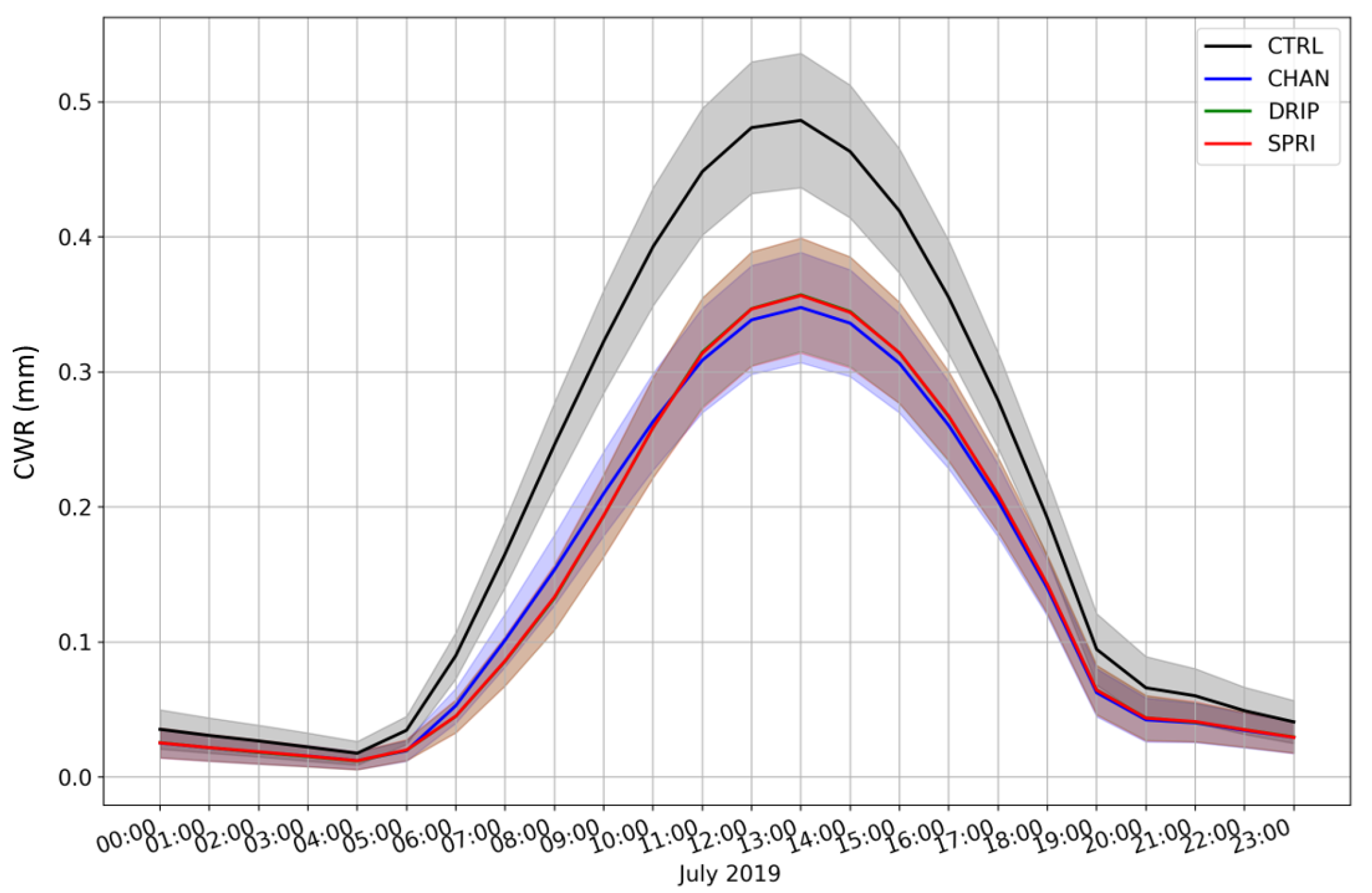
Due to the difficulty of measuring soil moisture at certain depths and with a spatio-temporal resolution suitable for agricultural application, the crop water requirement is a more common indicator of plant health. It represents the water needed to meet the consumption by the crop [
60], and is calculated as the difference between the potential evapotranspiration and the actual evapotranspiration. The result obtained for the diurnal cycle of July 2015 over the Po Valley irrigated area is shown in
Figure 10. As expected, irrigation reduces significantly the water deficit that is observed in the control simulation. All the irrigated runs shows similar behavior, and the small difference observed during the irrigation cycle (5–9 UTC) can be attributed to the irrigation method efficiency. The diurnal integrated crop water requirement is reduced from 4.821 mm/day of the control simulation to
mm/day for the irrigated ones. This value is comparable to the averaged input water applied by the model of 2.394 mm/day, after considering the irrigation mask weighting.
4.2. Potential Feedback to Heatwave
When soil moisture is considered, the feedback effects must be considered beyond the direct and most evident ones. In fact, soil moisture can play a crucial role in affecting the local atmospheric and climatic conditions. This feedback depends on the regional strength of the soil–atmosphere coupling. The studied region shows a very strong coupling, e.g., [
9,
28], which reflects on heat waves [
59]. As Miralles et al. [
59] discussed, prolonged periods of precipitation deficit favor heat wave formation. A decrease in evapotranspiration enhances a heat wave and can cause self-propagation and self-intensification. From the previously analysed results, both evapotranspiration and soil moisture were strongly affected by irrigation in this region. During the July 2015 heat wave, irrigation increased both variables up to 55% with respect to the simulation that did not consider the process. However, such an increase is not enough to disrupt the synoptic scale pattern and dissipate the heat wave conditions for the chosen case.
Irrigation assumes a more crucial role when the water applied is considered as separate from the hydrological cycle. In Miralles et al. [
59], soil moisture anomalies are strictly correlated to the precipitation, but such an assumption is not true in the case of irrigated land. In fact, soil moisture in that area is modulated by the irrigation water availability and application, which will depend on the source. While in extreme drought conditions the sources are affected by climatic conditions, this currently happens rarely. Only a few of the past years have been affected by a governmental irrigation reduction or halt for the whole area or parts of it [
48]. Therefore, the heat wave self-intensification and self-propagation processes, as described by Miralles et al. [
59], is less common in regions that are highly irrigated. In considering the coupling between atmosphere and soil, irrigation must be considered, as it might mitigate the actual strength.
4.3. Atmospheric Pollution
Analysing the results for the boundary layer, the diurnal cycle has been found to be affected in the irrigated run, more during the July heat wave. The height of the convective mixed layer is reduced by a third, from an averaged value of 1.5 km (in the control simulation) to less than 1 km (for case shown,
Figure 7b). Such a reduction impacts the atmospheric dynamics, as well as the convection, and this is analysed in depth in [
58]. However, these changes also affect the mixing height and the local dispersion. While in remote areas, such changes might not be relevant, the Po Valley region is highly inhabited and industrialized, and atmospheric pollution is a constant concern. Considering only the physical processes in boundary layer dispersion of air pollution, a reduction in the height causes an increase in the concentration. However, this conclusion can only be applied to passive hydrophobic atmospheric pollution components (e.g., some hydrophobic aerosols), as the chemistry processes must be considered as well. In the irrigated runs, the atmospheric moisture content is also affected, which affects chemical reactions as well as the interaction of hydrophilic aerosols.
The impact of such changes is not as simple as the previously described dynamical one. For the case of hydrophilic aerosols, the increase in water vapor might cause a higher activation rate as hygroscopic nuclei for cloud formation, or a radius increase that makes removal easier and reduces visibility. Such processes would lead to a decrease in their atmospheric content, which is the opposite effect of what is expected by the decrease in the mixing height. An other example could be for the tropospheric ozone, where both temperature and water vapor play an important role in regulating the reactions speed. Irrigation by decreasing the boundary layer height would increase the ozone content, and considering the chemistry, on one hand the cooler environment reduces the formation, but on the other hand, the increase in water vapor facilitates the formation.
Therefore, the overall impact of irrigation on air pollution might not be straightforward, but only considering basic processes it is expected to have some impacts. This study does not investigate the complex feedback effects on air pollution chemistry and dispersion, as WRF-ARW is not a suitable model. Also, the used resolution is too coarse to properly investigate the spatial and temporal scales of such processes. Therefore, this gives a possible starting point for further studies.
4.4. Heat Discomfort
Both temperature and humidity variables are generally used to assess heat discomfort [
61]. Changes in these quantities, especially during heat wave conditions, will affect the heat stress of both vegetation and humans, e.g., [
62,
63,
64,
65,
66,
67,
68]. Buzan et al. [
61] presents different indices that can be used to assess heat discomfort. Of the ones proposed, a physiological index is preferred to the others as it relates the impact of the meteorological variables on humans with the use of qualitative values. While these threshold values might not be representative of all the human population, they allow us to relate the complex biological response to the atmospheric environment. In particular, the Discomfort Index (DI, Equation (10), Buzan et al. [
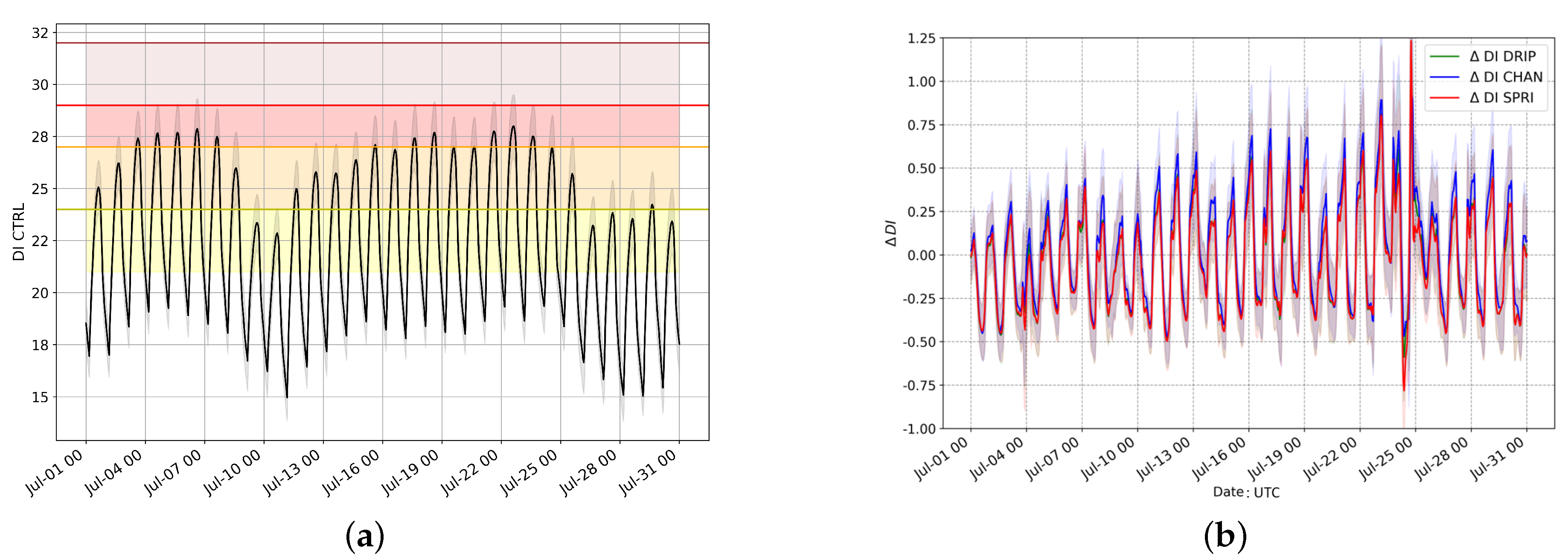
61]) combines, in a simple way, the atmospheric variables that are directly affected by irrigation, the 2-m temperature and the wet bulb temperature (which accounts for the relative humidity as well as the temperature). The threshold values are defined as follows: The control run obtains high values of DI for most of the period (
Figure 11a).
During the frontal passage of 9–10 July and 24–25 July, the average DI for the region is below 24 for the whole day. On the other hand, during the heat wave periods, the averaged values are always over 24 (so more than 50% of the population would be in discomfort). In the central part of both heat waves, the region has most of the population suffering (), and part of it in severe stress (the spatial standard deviation, ). In the nighttime, DI values decrease below the minimum threshold, even if for just few hours in the central part of the heat waves.
After subtracting the spatial fields of the control run from the irrigated case, the spatially averaged time-series is obtained as
Figure 11b. Firstly, the differences show a clear diurnal cycle similar to what obtained for the T2. In fact, midday values are decreased in the irrigated run, as might be expected. While a decrease of 0.5 in DI might not seem relevant if compared to the absolute value, it is to be remembered that each threshold contains 3 DI units. The same reasoning can be made for the increase in DI observed during the nighttime. In the first July heat wave, the nighttime increase is lower than the daytime decrease. The opposite behavior is observed for the second July heat wave (10 July to 24 July), with the nighttime increase over 0.5 for the whole period and peaks over 0.75 in the last part.
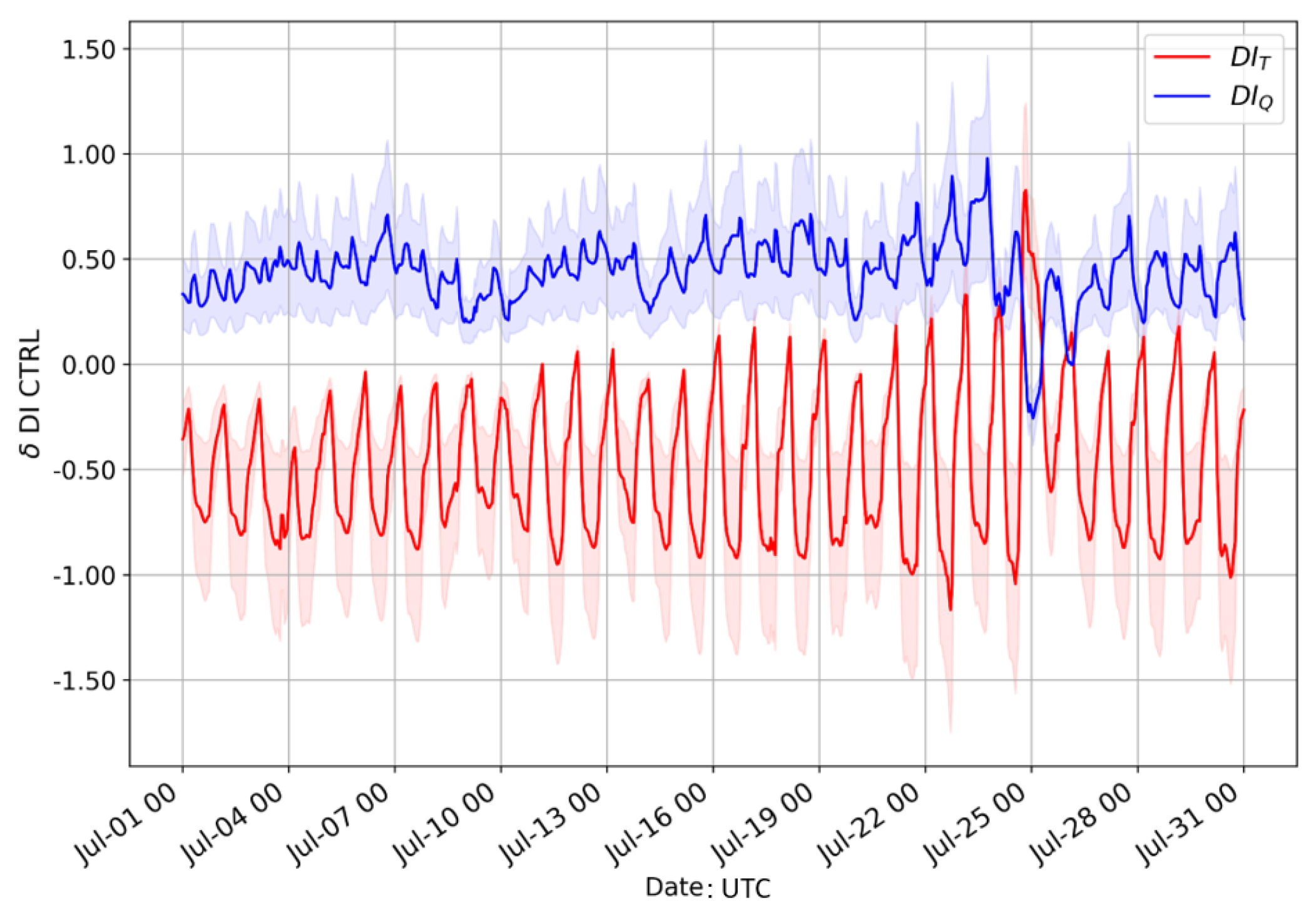
To differentiate the impact of decrease in temperature and increase in moisture, the contributions are separated. To do so, the irrigated temperature and the irrigated atmospheric moisture are used individually to compute the DI, called respectively
and
. To compare the obtained value, the time-series of the field-differences for the region are calculated. The results are shown separately in
Figure 12 below. As expected, the reduction of DI due to just the decrease in temperature would be higher than that obtained in
Figure 11b. This is because the increase in moisture contribution is non trivial, accounting for over 50% of the value. The increase of the nighttime discomfort index observed in the irrigated runs is caused mainly by the moisture part of the equation. In fact, while
has a strong diurnal cycle, with almost zero contribution during the nighttime, the atmospheric moisture has a lesser amplitude, with a more constant offset.
4.5. Remark on Results’ Interpretation
In interpreting the previously discussed results, it might be tempting to draw the conclusion that irrigation improves some aspects of the local environment, e.g., reduces the discomfort or affects the heat waves. In fact, some studies have presented irrigation as a geoengineering technique to mitigate some aspects [
59,
69,
70]. However, this is not the case for the simulations presented in this paper. In general, the irrigation parameterizations have been found to improve the simulations when compared against surface temperature stations, Moderate Resolution Imaging Spectroradiometer (MODIS) potential evapotranspiration and radar composite for some precipitation events [
43]. After the validation, the irrigated runs describe the reality and the control the potential reality in the situation of a non-irrigated Po Valley.
In a broader perspective, the control simulation might give insight for a heat wave situation in which the water resources are so depleted that irrigation cannot be sustained. For the chosen region, this situation has happened already in 2003 and 2012 [
48], where a winter drought caused low snow-pack in the Alpine region and lower summer river yields. Such situations are projected to become more common in future climate projections [
4], threatening irrigation by reducing the water amount available. This knowledge has to be combined with the increased projected water demand in most of the agricultural regions [
32]. Therefore, this effect also has to be added to the already modelled climate change signal for future projection, in highly irrigated regions. In fact, the lack of irrigation might further increase the temperature and enhance the heat waves helped by the soil-atmosphere feedback effect.
Further numerical studies must be performed for both current climate and sensitivity to future conditions in order to understand fully and quantify the irrigation signal and potential changes in it that may be affected by water resources. While this might not be crucial for the average summer conditions (as seen, June 2015 shows a small signal), it is important for extreme events. This must be considered only as a starting point for possible follow ups.
5. Conclusions
Previous studies investigated the effect of irrigation on the local climate, discussing its regional and climate condition dependence. Of particular interest is the impact of irrigation during heat wave conditions in areas where the soil–atmosphere coupling is strong, such as the Mediterranean region. Within the Mediterranean area, the northern Italy area was chosen due to its long historical use of irrigation (already widespread in the 15th century). In particular, the focus is on a summer season with an intense and prolonged heat wave period (July 2015) preceded by an average month (June 2015). To allow consideration of a potential irrigation-precipitation feedback [
9,
26], the WRF-ARW is run at a 3 km convection-permitting scale. In our previous studies, irrigation parameterizations have been developed and tested for the current period and region [
43]. With the current study, the impact of different synoptic states on the response of the local conditions is investigated. Later, the potential implications for the region were discussed.
To assess the impact of irrigation, a control run was used without the new parameterizations, which is the currently available WRF version 3.8.1. First, irrigation is found to drastically increase the soil moisture content of the first layer. The increase is up to 10–33% in June and up to 55% in July. This affected also the root zone (third level) soil moisture used by the plants, causing an increase of double the values obtained in the control simulation, where some areas reached the wilting point. This leads to a decrease in the crop water requirement in the irrigated runs of 50% in the diurnal integrated value with respect to the control simulation.
The increase in soil moisture might have an impact on the overall heat wave conditions and development, in the formulation of Miralles et al. [
59]. In fact, some irrigation has been found to decouple the soil moisture anomalies caused by the lack of precipitation and strong evapotranspiration in heat-stressed periods. Therefore, this might affect the self-propagation and self-intensification mechanism [
59], when highly irrigated regions are considered. However, for the case study, irrigation does not disrupt the heat wave conditions but just modulates the intensity. This can be related to the irrigation extent that is not enough to sustain this feedback.
Differences in soil moisture then impact the partition of the surface fluxes differently for each month, causing the upward moisture flux to increase more in July than June (respectively, 15% and 52%). The increase in the moisture flux causes the 2-m moisture content to rise differently in the two months, respectively up to 10% and 25–50%. However, the partition of the fluxes changes, and the sensible heat fluxes decrease 13% in June and 23% in July. This reflects differently on the 2-m temperature, as the variation depends on the time of the day, with a maximum change during the central hours. In fact, this study finds that the maximum daily temperature is the most affected quantity with a reduction up to 2.5–3 K with respect to the control (July). Due to the lesser changes in June, also the maximum daily temperature is less affected, with a decrease between 0.75–1 K.
As previously mentioned, the almost zero nighttime impact of irrigation on the sensible heat fluxes is seen from the lack of spatial changes in the daily minimum temperatures. Such changes in temperature and atmospheric moisture are found to affect the heat discomfort in the region, which is densely populated. Quantifying this impact on the population with the Discomfort Index (DI), the control simulation’s main core of July heat waves period register values that indicates that most of the population is in discomfort (), with peaks of severe stress. In the irrigated runs, DI is reduced during the daytime up to 0.5, which brings the index near to the threshold value. However, the nighttime shows an increase in DI, which is found to be related to the moistening of the air caused by irrigation, that does not have as strong a diurnal cycle as the decrease in temperature.
The changes in the surface values of temperature and moisture propagate vertically, and have a diurnal cycle as well. As expected, such changes are different in June and July, with higher magnitude in the latter. Considering the potential temperature, the irrigated runs show a decrease within the lower troposphere, with a clear diurnal cycle. Such changes affect the boundary layer height causing it to decrease, on average, from 1.5 km to 1 km. Such a decrease might have an impact on the atmospheric air pollution, that for the region is an on-going problem because a lower PBL height reduces the mixing length, which, in turn, might increase the concentration of atmospheric pollution components. This is simplified consideration that is true only for passive non-chemically reactive components. As a side note, the increase in water vapor mixing ratio, which has a vertical pattern similar to the changes in the boundary layer structure, might also affect the chemistry of the pollutant reactions.
All the changes observed comparing the irrigated runs to the control are caused by the irrigation, through the soil moisture differences. This was done by calculating the correlation between the differences in the time-series of a set of variables. It is easier to prove the relationships between soil moisture and the surface fluxes and 2-m temperature, as they have high correlation. Interestingly, the soil moisture is found to affect the thermodynamics of the air masses by changing the boundary layer averaged mixing ratio, that lowers both the lifting condensation level (LCL) and level of free convection (LFC).
In the interpretation of the results and from the validated simulations we can assess that in case irrigation is halted, the control simulation might be a probable local climatic state. For the considered region, this has happened already in drought winter years that caused very low snow-pack and consequent low yield (e.g., 2003). However, the implications go beyond the past cases, as such reductions are projected to be more frequent under future climate projections. Therefore, the irrigation impact must be assessed in the current climate to understand possible repercussions for the future. However, all conclusions here are based on theoretical considerations considering one summer condition, which included both a normal month and two heat waves. To quantify them statistically, more periods should be simulated to better sample the current climate impact, and several ensemble simulations of pseudo global warming cases should be performed. This was not in the scope of the present study but would be a valuable extension.


