Abstract
Due to the development of industrialization and urbanization, secondary pollution is becoming increasingly serious in the Yangtze River Delta. Volatile organic compounds (VOCs) are key precursors of the near-surface ozone, secondary organic aerosol (SOA), and other secondary pollutants. In this study, we chose a serious ozone pollution period (01 May–31 July 2017) in Jinshan, which is a petrochemical and industrial area in Shanghai. We explored the VOCs distribution characteristics and contribution to secondary pollutants via constructing a regional network based on wind patterns. We determined that dense pollutants were accumulated at adjacent sites under local circulation (LC), and pollution from petrochemical discharge was more serious than industry for all sites under southeast (SE) wind. We also found that cyclopentane, o-xylene, m/p-xylene, 1-3-butadiene, and 1-hexene were priority-controlled species as they were most vital to form secondary pollutants. This study proves that regional network analysis can be successfully applied to explore pollution characteristics and regional secondary pollutants formation.
1. Introduction
Volatile organic compounds (VOCs) are major participants in atmospheric photochemical processes and key precursors for the formation of near-surface ozone, secondary organic aerosol (SOA), and other secondary pollutants [1,2]. VOCs can be oxidized by OH radicals, ozone radicals, and nitrite radicals (NO3), initiating the HOx cycle in the ambient atmosphere, which affects the concentration of HOx, and consequently affects the lifetime of other substances [3]; therefore, VOCs have direct and indirect detrimental impacts on climate, photochemical smog, the ecosystem, and human health [4,5,6,7]. Owing to the rapid development of industrialization and urbanization, pollution levels exceeded the World Health Organization (WHO) air quality criteria on more than 250 days in China during 2011 [8]. The total amount of anthropogenic VOCs discharged in China was 25.03 million tons in 2015 [9], and air pollution has shifted from single to compound photochemical pollution. Industrial emissions, especially unorganized solvent, paint, and petrochemical emissions, account for the largest sources of anthropogenic VOCs [10,11,12].
As for regional emissions, the Yangtze River Delta (YRD) not only shows the highest emissions, but also has the highest contribution to ozone and SOA formation nationwide [9,13]. Huang et al. [10] found that high ozone formation potential (OFP) values are mainly gathered in industrial areas along the Yangtze River and around Hangzhou Bay. Jinshan District in Shanghai is located in a highly industrialized area, and these industrial production activities result in large VOCs emissions with high chemical reactivities and diverse components [14], which have a significant influence on air quality. It was found that the number of days that ozone concentrations exceed the national ambient air quality standards is highest in Jinshan District compared to other districts in Shanghai [15].
In addition to emissions, air quality is also reliant on meteorological conditions. Cheng et al. [16] found that land–sea breeze flow dominates the redistribution of locally produced ozone via simulations. Angevine et al. [17] believed that air pollution episodes in northern New England are often caused by the transport of pollutants driven by the wind. The interaction between emissions and wind fields can determine the overall air quality of a region [18].
Although ozone pollution is a regional pollution problem, previous studies only focused on individual sites, thereby lacking the concept of combining the analysis of regional sites [11,19,20]. Since Shanghai is a VOC-limited region, the control of VOCs is essential to prevent ozone formation [21,22]. In order to characterize the VOCs in Jinshan District and explore their effects on ozone pollution, this study chose the high ozone pollution months (from 01 May 1 to 31 July 2017) to conduct a combined analysis via densely distributed stations by constructing a regional network based on wind patterns. We investigated the VOCs profiles, characterized the pollution features with indicators, and calculated ozone formation and SOA formation for consumed VOCs during transportation. Through this analysis, we obtained a simple mechanism for regional analysis with high spatiotemporal resolution data, which could be used to reveal how major pollution emission sources affect the surrounding areas. It will be helpful to provide support for VOCs emission control in this region.
2. Experiments
2.1. Sampling Sites and Period
Jinshan District is in the center of an economic zone that is comprised of Shanghai, Hangzhou, Ningbo, and the Zhoushan Islands, and it is the southwest gateway to Shanghai. There are two main emission sources in this region, namely Sinopec Shanghai Petrochemical Co., Ltd., which is China’s largest petrochemical industrial complex (hereafter called the Complex), and the Jinshan Second Industrial Zone. The Complex produces aviation kerosene, gasoline diesel, aromatic olefins, etc., and emits VOCs via oil refineries, leakage of storage tanks, and water treatment processes [23]. The Jinshan Second Industrial Zone contains a large number of industries, such as electronic information engineering, machinery manufacturing, biomedicine, iron and steel plants, synthetic/new materials, cement, new energy, and research and development (R&D) technology.
As shown in Figure 1, there were six monitoring sites, namely Xinlian (XL), Guomao (GM), Zhangqiao (ZQ), Shihua Street (SHJD), Weiliu (WL), and Xincheng (XC), in Jinshan District that were governed by the Jinshan Environmental Monitoring Station. WL is in the zone of the Complex and represents the Complex source. XL is the northwest border station of the Second Industrial Zone and directly affected by the petrochemical industrial area. GM is the northeast border station of the Second Industrial Zone, XL and GM are both in the north of the Complex, and ZQ is a rural site in the northwest of the Complex and Second Industrial Zone. SHJD and XC are urban sites that are located in the residential area of Jinshan New Town and near Hangzhou Bay. The sampler inlets of these six sites are on the rooftops of buildings with heights of 15–20 m.
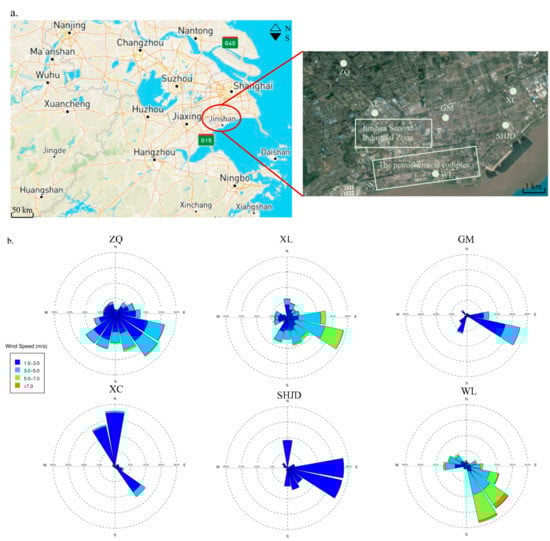
Figure 1.
(a) Location of six sites in Jinshan District; (b) wind rose of all sites during May and July. XL: Xinlian; GM: Guomao; ZQ: Zhangqiao; SHJD: Shihua Street; WL: Weiliu; XC: Xincheng.
Observations were conducted from 01 May 1 to 31 July 2017, which was a heavy ozone pollution period. Trace gases (such as ozone, sulfur dioxide, hydrogen sulfide, nitric oxide, nitrogen dioxide, ammonia, and carbon monoxide), VOCs (non-methane hydrocarbons (NMHCs)), and meteorological parameters (wind speed, wind direction, temperature, and relative humility) were obtained during the observation period (Table 1).

Table 1.
Instruments used in the observation.
2.2. Instrument Quality Control
VOCs were measured with a gas chromatograph equipped with two detectors, a photoionization detector (PID) and a flame ionization detector (FID). Samples were brought into the pre-concentration unit; with the help of an indirect piston system 35 mL sample gas was preconcentrated on a small packed column. The pre-concentration tube can be cooled to −10 °C by radiation to absorb VOCs with boiling points below 20 °C. It can also be purged with carrier gas (nitrogen) to remove oxygen and water. Concentrated samples were flushed through the column (length: 30 m; inner diameter: 0.53 mm) and due to the different boiling points, various VOCs were separated; compounds with lower boiling point eluted earlier from the column than compounds with a higher boiling point. After eluting from the column, the compounds were fed into the detector, whereby a digital signal was generated that was proportional to the concentration. The PID achieves a high resolution and allows for the measurement of very low concentrations (down to 150 ppt); it is traditionally favored for continuous benzene, toluene, ethylbenzene, and xylenes (BTEX) monitoring [24], whereas the FID’s sensitivity makes it suitable for the low ppb to ppm range, making it more popular in recent years [25,26]. Therefore, the combination of a PID and a FID gave the opportunity to monitor complex mixtures satisfactorily. When a chromatogram was recorded, individual VOCs were identified by their retention time and quantified by integrating their individual peak. A calibration was used to determine the conversion factor for automatic calculation of concentrations from area values. To conduct the calibration, measurements of calibration gas in the desired dilutions with three repetitions for each set of concentrations was needed; then the conversion factor was determined. To verify the accuracy of the GC955, a single-point calibration (10 ppbv) was conducted every 2 weeks and a multi-point calibration (at least five points) was conducted every quarter; the correlation coefficient R2 needed to be larger than 0.99. The detection limit of GC955 is 0.1 nmol/mol (benzene) and the reproducibility is below 3% for 1 ppb benzene. The detectors and sampling tubes were cleaned twice per year. The preconcentration tube, carrier gas filter, ten-way valve membrane, and drying tube were replaced once per year.
Auto Met Station WS500-UMB was used to obtain the meteorological data (wind speed and direction data, temperature, relative humidity). Wind speed and direction were measured by an ultrasonic sensor with resolution of 0.1 m/s and 0.1° separately.
All monitoring data were measured according to air quality standards (HJ644-2013). Briefly, the data capture rates for these instruments were over 95% with a data efficiency of over 85%.
2.3. Categorization of Surface Wind Patterns
To systematically analyze the VOCs characteristics in the Jinshan District with meteorology, we subdivided the wind into four typical patterns based on the meteorological data from the Jinshan Environmental Monitoring Station. The categorization was defined by diurnal variation in wind speed and direction based on Chen et al. [18]. Shanghai’s climate is subtropical monsoon, and wind conditions are highly seasonal; the dominant wind flow pattern is southeast monsoonal in summer, and local circulation (LC) is common in the coastal region. Two other wind patterns were identified to cover the wind coming from all directions.
Local circulation is regional circulation at meso and local scales, such as land–sea breeze and mountain–valley winds. The LC was characterized by wind direction that changed by more than 90° within 24 h; the wind speed was comparatively low (the daily average value was less than 3 m·s−1), but the wind speed was higher in the daytime compared to nighttime [27]. It played an important role in determining the distribution of air pollutants, as high pollution events usually occur under this wind flow [18,28].
For southeast wind (SE), southwest wind (SW), and north wind (N), the wind direction changed within 90° in 24 h with relatively high wind speed (the daily average exceeded 3 m·s−1) and mainly in the direction ranges of 60°–170°, 170°–270°, and 280°–60°, respectively. The range did not need to be exactly the same as the convention [18], as this was determined to make sure that one pollution source was in the scope of one wind pattern for most sites. Owing to the high wind speed, pollutants can affect downwind sites significantly.
All the days during the observation period could be accurately categorized into these four typical wind patterns.
3. Results
3.1. Wind Fields in Jinshan District
The statistical frequencies of wind directions at each site are shown in Table 2. LC was the dominant wind pattern during the observation period, followed by SE. SW and N wind accounted for about 10% of all wind directions at all sites, except for XC, where the frequency of north wind accounted for 22%. Except for WL, the contribution from the SE decreased from 43% at SHJD (coastal) to 22% at ZQ (inland), thereby suggesting that SE had more impact on the coast than inland.
Table 2.
Proportions for various wind flow patterns at each site during May and July. LC: local circulation; SE: southeast wind; SW: southwest wind; N: north wind.
To construct a regional network utilizing the advantage of densely distributed stations, the analysis of wind patterns for the whole Jinshan District area was necessary. The wind field of Jinshan was analyzed in a way that if the daily wind patterns of more than four of the six stations were the same, then the wind pattern of Jinshan District was determined to be the same. Otherwise, the wind in Jinshan District could not be classified into any typical pattern, then it was defined as ambiguous instead. The data showed that 81 of 92 days had unanimous district-wide wind patterns. Figure 2 displays the frequency distribution of monthly wind patterns in Jinshan District, which shows that the occurrences of LC and ambiguous patterns increased from May to July; in contrast, the percentage of the SE decreased from May to July, which meant that the wind direction changed more frequently and widely in July. Overall, LC (50%) and SE (28%) flows were the most frequently occurring wind patterns during the observation period in the Jinshan District area.
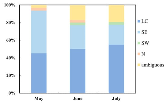
Figure 2.
Frequency distribution of wind patterns in Jinshan District during May and July. Ambiguous means wind cannot be sorted to four typical patterns.
3.2. Statistic Analysis for Wind and VOCs Concentrations
In this study, we represented total VOCs (TVOCs) using the hourly resolution data of 56 non-methane hydrocarbons (NMHCs) [29]. A Pearson correlation analysis of wind speed and total VOCs concentrations was carried out to illustrate their relationships based on three months’ hourly data (Table 3). The negative correlation showed that high pollution events usually occur under low wind speed; the relatively weak correlations were reasonable since the concentrations of pollutants were also affected by discharge, surface terrain, etc. The counts of occurrences within certain VOCs concentration ranges under each range of wind direction were shown in Figure 3, which revealed that the high pollution events occurred most under SE and SW for ZQ and XL; SW for GM; N for XC; SW for SHJD.
Table 3.
Pearson correlation coefficient of wind speed and total volatile organic compound (TVOCs) concentrations.
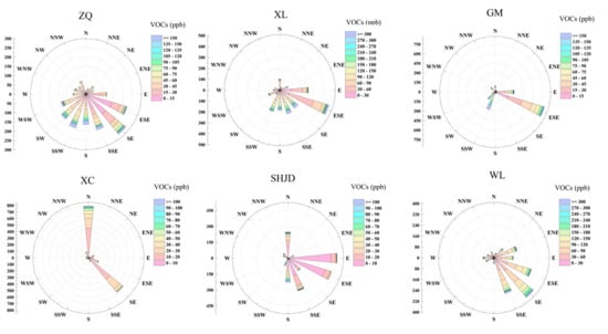
Figure 3.
General relationship between wind direction and total VOCs concentrations based on three months’ hourly data. Colors represent different VOCs concentrations; radius represents the counts of occurrences within certain VOCs concentration ranges under each range of wind direction.
Nevertheless, these simple statistical analyses may not demonstrate the influence on VOCs concentrations comprehensively, thus a detailed analysis was carried out as follows.
3.3. Influence of the Four Wind Patterns on VOCs
The diurnal variation in VOCs could be successfully explained via wind patterns in 62 out of 92 cases. Jia et al. [30] reported small inter-city VOCs concentration changes in urban, suburban, and industrial neighborhoods; unlike their research, the results from the six sites in this study showed clear differences. Here we selected one case under each wind pattern to demonstrate the effect of surface wind on the distribution of air pollutants from major sources as shown in Figure 4, which is in line with the statistical analysis.
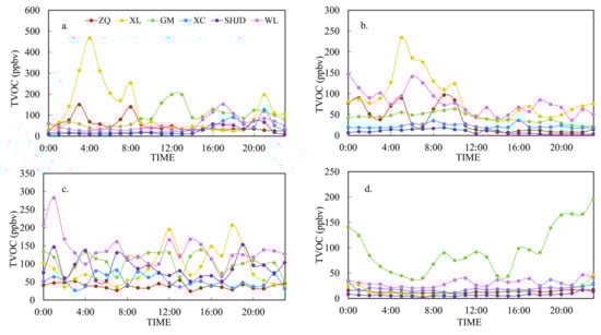
Figure 4.
Typical cases of VOCs diurnal variation under different wind patterns. (a) LC pattern on 9 June; (b) southeast wind flow on 1 May; (c) southwest wind flow on 25 June; (d) north flow on 24 May.
LC was the guiding wind pattern during the observation period, and we chose 09 June to illustrate this, during which the wind direction changed frequently and largely. The wind directions at SHJD and GM swung from SE to SW at 14:00 and 10:00, respectively, carrying petrochemical pollution plumes from the Complex and accompanying the elevation of the mixing ratios. Before 10:00, the wind directions at ZQ and XL were SE; owing to the influence of the petrochemical area, the VOCs concentrations were significantly higher than those later in the day. The variation trend at ZQ before 10:00 was analogous to that at XL, thereby indicating that plumes may be derived from XL when the wind direction was SE. Such representative cases took place in 32 out of 47 days, thereby showing that the pollution conditions were sensitive to wind direction.
We chose 01 May to represent SE, and both wind speed and direction were less variable on that day. The plume from the Complex and XL hit ZQ, so it was directly affected by compound pollution of the Complex and the industrial area under SE, resulting in high VOCs concentrations among SE, SW, and N. The decrease in VOCs concentrations was related to the wind turning to 100° at 14:00. GM was only partially contaminated by petrochemicals, which led to its moderate VOCs concentration level. Located upwind of the Complex and industrial area, SHJD and XC had extremely low VOCs concentrations and smooth diurnal variation; the disparity was that the wind directions at SHJD and XC were 100° and 145°, respectively, so XC might have been slightly influenced by the residential area of Jinshan New Town. Such representative cases took place in 18 out of 31 days.
It was determined that 25 June was the only typical and explainable case under SW. SHJD and GM showed relatively higher VOCs concentrations compared to those under other wind patterns, especially for SHJD, which had a variation trend that was mostly in accordance with that of WL. The VOCs mixing ratio at ZQ was maintained at the lowest level, thereby revealing less impact from the petrochemical areas. Such representative cases took place in 1 out of 2 days.
The north wind carried less contaminated air from the main city of Shanghai, and all sites except for GM showed low VOCs concentration levels (<50 ppbv). Such representative cases took place in 2 out of 2 days. To demonstrate the high mixing ratio at GM, we calculated the ratios of xylene/benzene (X/B) and benzene/toluene (B/T) to determine the aging of the air mass. Benzene, toluene, ethylbenzene, and xylenes (BTEX) are emitted from similar sources, but they have different photochemical reactivities. The photochemical lifetimes of BTEX in the presence of OH radicals are 12.5 d, 2 d, 23 h, and 7.8 h, respectively [31]. According to Liu et al. [32], when X/B > 1.1 and B/T < 0.4, the air mass is considered fresh. The ratios of X/B and B/T at GM were 5.8 and 0.2, respectively. Additionally, on 24 May, the most abundant VOCs at GM were iso-butane, n-butane, and propane, which mainly originated from liquefied petroleum gas (LPG) usage, diesel exhaust, and natural gas usage [6,33,34], thereby implying that the high level of VOCs resulted from local emissions from residents’ usage of household fuel and motorcycles around the site.
3.4. VOCs Fingerprint Profiles Analysis
VOCs fingerprint profiles offered a more sophisticated assessment tool to interpret the source–receptor relationship. Situated inside the Complex and surrounded by highly dense facilities, WL represented the petrochemical emission source. As the northwestern boundary of the Second Industrial Zone, XL was most directly and severely affected, and represented the source of industrial emissions. Other sites were receptor sites of the Complex and the industrial area under different wind patterns. This is also shown in Figure 4, where the VOCs concentrations at the sources were obviously higher than those at the receptor sites. In addition, other local emissions and background levels were negligible compared to these two major sources [35], so the concentration level and chemical composition at WL and XL could represent the petrochemical and industrial emissions.
The averaged profiles of the most abundant VOCs species revealed the overall level during the observation period, as shown in Figure 5a. At WL, ethylene accounted for the largest proportion (18.4%) of VOCs concentrations, followed by propylene (17.9%), ethane (9.3%), cyclopentane (8.8%), propane (4.9%), and isopentane (4.2%). Benzene and toluene also played a non-negligible part with proportions of 1.8% and 2.1%, respectively. These species were products from petrochemical processes [5,36]. Among these species, C4–C5 alkanes were mainly emitted from gasoline manufacturing processes, and C6–C7 alkenes were emitted from diesel fuel production processes [37]. This result was similar to that in Taiwan [29], except for cyclopentane, which mainly originated from ethylene cracking, reforming naphtha, and oilfield condensation [38]. Both the petrochemical and industrial areas emitted large amounts of m/p-xylene, benzene, and toluene, which were in line with the high concentrations at XL (m/p-xylene: 11.7 ppbv, benzene: 5.5 ppbv, toluene: 6.1 ppbv) [11,36,39].
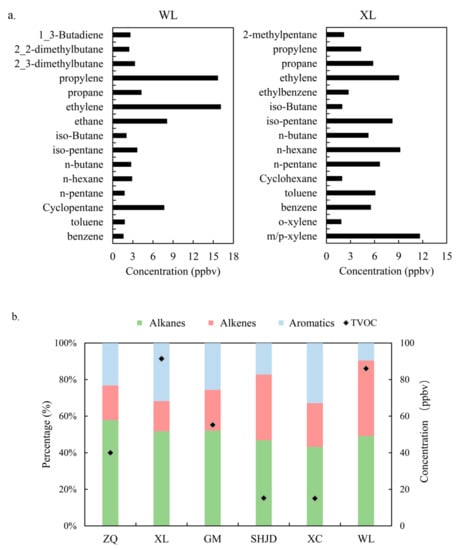
Figure 5.
(a) The mean concentrations of the 15 most abundant VOCs of WL and XL; (b) the proportion of alkanes, alkenes, and aromatics at monitoring sites from May to July.
Given the particularities of the area studied, namely, the prominent sources were the petrochemical and industrial areas, vehicular emissions had less impact (Section 3.6), alkanes and alkenes were mainly produced from the petrochemical processes, and aromatics derived from industries using solvents and paint [11,40,41,42,43]. Alkanes are relatively stable [44] and have smaller photochemical reactivities compared to those of alkenes and aromatics; thus, they could be transported over long distances. Thus, the proportions of alkanes were largest and varied little among all sites, as presented in Figure 5b. The transport of alkenes was accompanied with consumption; therefore, the alkene fractions were inversely proportional to the distances from the petrochemical emission source [43]. The fractions of aromatics were relatively higher at XL (32%) and XC (33%) and were extremely low at WL (10%). As for the VOCs concentrations, those at XL and WL were obviously higher than those at other sites with the values of 91 ppbv and 86 ppbv, respectively. SHJD and XC, lying in Jinshan New Town, had the lightest pollution and the lowest VOCs concentrations among all monitoring sites.
The above description shows the VOCs compositions over the long-term at two source sites and four receptor sites, which provided a baseline level to illustrate the changes in VOCs constitutions under a particular wind pattern. Since the receptor sites were severely contaminated under LC, SE, and SW, and there were significant discrepancies of pollution characteristics at downwind sites under SE and SW, the VOCs compositions under SE and SW were emphasized. It is inferred from Figure 5a that the major contained VOCs species were consistent, even though the proportions changed significantly under SE and SW. WL, which was a petrochemical emission source site, showed large amounts of propane, propylene, n/iso-butane, ethylene, and ethane. The increase in 1-3-butadiene, an important raw material in the petrochemical and manufacturing industries [45], was caused by different processes of oil refineries and the products concerned. WL, XL, and ZQ showed large amounts of ethylene under the SE pattern, thereby reflecting the impact of wind on pollutants transportation and distribution. The profiles at SHJD showed a significant contrast under SE and SW. Compared with the low VOCs concentrations under SE, the concentrations of ethylene, ethane, propylene, and propane increased significantly under the SW pattern. Oppositely, the proportions of individual VOCs species were even under SW at both GM and XC. The VOCs fingerprint profiles in Figure 6a manifest an evident source–receptor relationship, suggesting that under the SW flow, GM and XC encountered plumes carrying both petrochemical and industrial pollutants, whereas SHJD was only affected by the petrochemical area, which largely missed the plumes from industrial area.
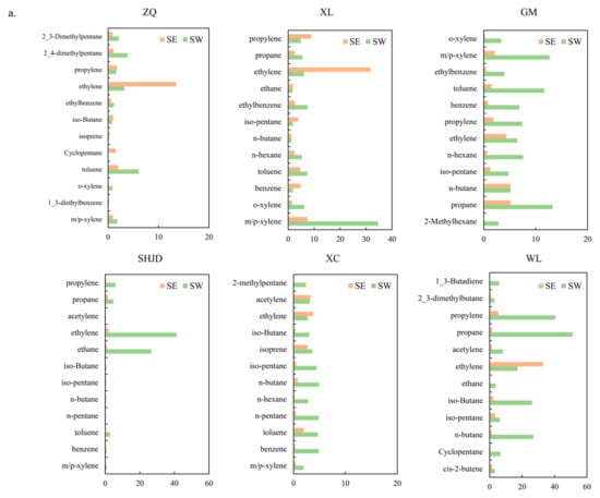
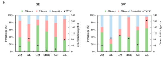
Figure 6.
(a) The 12 most abundant 12 VOCs; (b) the fraction of alkanes, alkenes, and aromatics under SE (1 May) and SW flow (25 June).
The contradistinction of fractions of alkanes, alkenes, and aromatics at the six sites under SE and SW is presented in Figure 6b to certify that the pollutant species were divergent under SE and SW. The proportions of aromatics at ZQ, XL, GM, and XC increased within the range of 10% to 42% under SW compared to SE because of the effect of industries using solvents. The percentage of alkenes at SHJD increased from 6% under SE to 15% under SW because the Complex emitted large amounts of alkenes. The change at WL might have been because different parts of the petrochemical plant were actuated. Concentrations of TVOCs did not vary much under SE and SW at ZQ or XL, yet they had an apparent increase within the range of 28–127 ppbv at GM, SHJD, and XC under SW flow.
3.5. VOCs Ozone Formation Potentials
During the observations, the 8 h daily maximum ozone reached up to 365 μg·m−3, which was the highest over the whole year. The average summer temperature with high humidity reached 30 °C and showed typical summer characteristics that facilitated photochemical reactions. This region was severely polluted under LC, SE, and SW, but this study focused on analyzing the relationship between pollution sources and downwind sites. SE and SW occupied nearly half of the observation period, and the ozone formation was analyzed under these conditions. The specific top VOCs ranked by their contribution to ozone formation are shown in Figure 7, which were evaluated by ozone formation potential (OFP) calculated by Equation (1). The maximum incremental reactivity (MIR) values were obtained from Carter [46].
where i refers to individual VOC.
OFP (i) = concentration (i) × MIR coefficient (i)
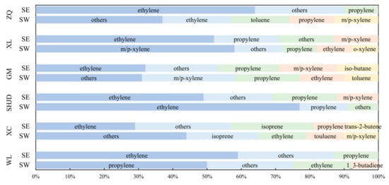
Figure 7.
The most important VOCs of ozone formation potential (OFP) contribution under SE and SW.
Alkanes had minimal contribution to ozone generation because of weak photochemical reactivities; alkenes and aromatic hydrocarbons with strong reactivities contributed more to the production of ozone [47,48]. The OFP values of ethylene and propylene occupied a significant proportion under all wind patterns and at all sites because of their high emission levels and high MIR values. This was obviously different from the urban atmosphere with aromatics as the main active component [43,49,50]. When plumes from the industrial area influenced the sites, namely at ZQ, XL under SE and GM under SW, m/p-xylene, o-xylene, and toluene contributed more to ozone formation. The dominant species with the highest OFP values were identical to those determined by An et al. [51] in an industrial area in the YRD. Owing to the abundant forest resources and strong solar radiation, plants emitted large quantities of isoprene, whose OFP ranked high at XC. Due to isoprene’s short lifetime of 1.4 h, it cannot be transported to other sites especially under SE and SW, making it not a vital ozone precursor at other sites. Isobutane emitted by both the Complex and household fuel at GM was also responsible for ozone formation.
3.6. VOCs Indicators Analysis
To further explain what type of pollution had a greater impact and the concrete pollution extent at each station under each wind flow, we selected indicators to distinguish petrochemical, industrial, and vehicular emissions based on the analysis of VOCs fingerprint profiles. Ethylene and propylene are two commonly used indexes for petroleum manufacturing processes [5,29]. Moreover, as shown in Figure 8, in cases affected and unaffected by the Complex, there was a clear boundary of the concentration of ethylene (ethylene = 3). The average values of ethylene were 5.9, 9.4, 7.3, 4.8, 2.1, and 20 at ZQ, XL, GM, SHJD, XC, and WL, respectively, which were correlated with the distances to WL under SE and SW flows. Among the most abundant VOCs at XL, ethylene, isopentane, n-pentane, propane, and propylene mainly originated from petroleum refinery processes; n-hexane, ethylbenzene, and o-xylene were mostly sourced from industry [52,53], whereas ethylbenzene was the only VOC that was not emitted by the Complex with a comparatively long chemical lifetime of 23 h. A critical line that separated the affected and unaffected cases could also be drawn, so the value was set at 1 for ethylbenzene. As for vehicular emissions, T/B is widely used to determine the vehicular exhaust contribution [29,32,34,54], and it is generally considered that a T/B of less than 2 implies significant emissions from motor vehicles. Given that ethylene > 3, ethylbenzene > 1, and T/B < 2 meant being affected by the Complex, industry, and vehicles separately, the influence on each site could be quantified as the time fraction for the hourly data at the given site under each wind pattern satisfying the inequality conditions, hereafter called the percent time of influence (TI%) [29]. Table 4 shows such percentage under the four typical wind patterns.
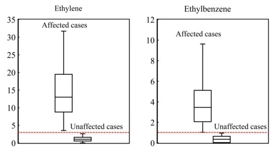
Figure 8.
The range of ethylene and ethylbenzene under affected and unaffected cases.
Table 4.
The percentage influenced by the Complex, industrial area, and vehicle emissions under different wind patterns.
Note that the reason why we did not choose a ratio (such as ethylene/acetylene) to reduce the effects of vehicular emissions was that the vehicular exhaust in the studied area was too weak. Chang et al. [55] showed that trans-2-pentene, cis-2-pentene, and acetylene are mainly derived from vehicular exhaust due to incomplete combustion, and they are widely used as the denominators [56]. However, these VOCs concentrations were too low to be used as denominators in our study. Taking trans-2-pentene as an example, the average concentrations at each station were 0.40 (XL), 0.07 (ZQ), 0.36 (GM), 0.01 (SHJD), 0.04 (XC), and 0.38 (WL). The ratio would be abnormally large if these VOCs were chosen as denominators. The ratio could not represent the real pollution condition, especially when the numerator (ethylene or ethylbenzene) was also small, yet the ratio was large. Thus, we could not use ratios as indicators.
Due to the low wind speed and diversification of wind directions under LC, dense pollutants were not transported far, and were accumulated at adjacent sites. Therefore, XL and GM were severely polluted by the Complex and industrial area with the highest TI% of 86%. The high industrial TI% of 60% at ZQ might have been related to the SuiLun Industrial Zone located 3 km southwest. The comparatively low TI% values at SHJD and XC were due to the longer distances from the sources, and the wind direction was irrelevant in excessive cases.
Under SE flow, pollution from petrochemical discharge was more serious than that from industrial zones for all sites, which coincided with the VOCs profile analysis. When ethylene at XC exceeded 3, the wind was more southerly compared to that at other times, namely it could incur part of the plume from the Complex. GM was slightly influenced by the industries when the wind direction was approximately 190° hours before SE flow; yet SHJD and XC were free from industrial pollution.
Under SW flow, SHJD was only affected by the Complex, which completely let plumes slip from the industrial zone, suggesting that SHJD was not aligned with the wind flow. GM and XC suffered from more pollution from industries compared to that from the Complex. The extremely high contamination from industries at XL (TI% = 100%) was not only because the site was positioned inside the Second Industrial Zone, but also because of the SuiLun Industrial Zone. Moreover, the southeast wind of the previous night (July 8) transported the pollutants to the northwest, and the southwesterly wind on July 9 transported the pollutants back, resulting in heavy contamination from the Complex and industry.
Under north flow, only XL and GM showed high TI%. They were both boundaries of the Second Industrial Zone, so it made sense that they were influenced by industrial pollution. In addition, the wind direction turned to 260° for several hours at XL on 07 June and elevated the mixing ratio of ethylene. As for GM, the concentration of ethylene surpassed 3 the entire day on 24 May, as mentioned in Section 3.3, and local emissions caused the high pollution level. With regard to other sites, their moments over the critical line were the same under winds at 270°, which was when SHJD and XC could be affected by the industrial zone but not by the Complex.
Vehicular exhaust is considered the major contributor to ambient VOCs in urban areas [37]. In contrast, Jinshan District was only slightly influenced by traffic emissions. Under north wind, the plumes from Shanghai main city resulted in slightly higher TI% of vehicles at ZQ, XL, and GM of 8% to 17%. Meanwhile, SHJD and XC were inside Jinshan New Town, and the ratio did not vary much under different wind patterns. High wind speed caused the low TI% at SHJD (0%) and XC (2%) under SE flow. The pollutants produced inside the town were transferred downwind, which was why the high values of ozone often appeared on the edge of the city or even in the suburbs [57].
4. Discussion
OH is the most important oxidant in the atmosphere, and trace gases are mainly converted or removed by reactions with OH [58]. Discharged VOCs have photochemical oxidation reactions with OH radicals, ozone, and NO3 radicals [2,59], but reactions with OH radicals are the leading photochemical loss for alkanes and aromatics [60], which form ozone and SOA. Most studies only calculated the OFP on the basis of the VOCs concentrations at the sampling sites and showed no consideration of the concentrations of ozone and SOA produced by VOCs during transportation and the quantitative influence of consumed VOCs on ozone and SOA formation. Thus, this study calculated OH exposure and VOCs consumption while being transported. Although OH radicals were not measured in this study, the OH exposure could be estimated from the decline in concentration of VOCs by Equation (2) derived from ct=co e−ki[OH]t [61,62], after correcting for physical dilution:
where ci(s) refers to the original concentration at the source site (ppbv), which is the highest value during the nighttime at WL when photochemical reactions are considered to be the weakest, and consequently are most reflective of the initial emissions [63]. To eliminate the effects of upwind concentration, we only discussed the cases where WL was the upwind site, namely under SE and SW. The background VOCs level was 29.97 ppbv in Shanghai [35]; thus, it could be ignored compared to the high emission at WL. ci(r) refers to the concentration at receptor sites (ppbv); D(t) refers to the dilution factors; OH·∆t·ki denotes OH exposure; and ki denotes the reaction rate constant with OH radicals (10−12 cm3·molecule−1·s−1) [64]. Taking ki as the abscissa and ln[(ci(r)⁄ci(s)] as the ordinate, OH·∆t and D(t) could be obtained for each hour during 9:00–18:00 from the slope and intercept of the regression. We chose VOCs that could satisfy the following parameters to obtain the regression: (1) the concentration in the atmosphere is relatively high, and the measurement is accurate; (2) a larger reactive activity range is covered; and (3) the background concentration is low. These selected VOCs’ KOH ranged from 1.22 10−12 cm3·molecule−1·s−1 (benzene) to 30 (propylene) 10−12 cm3 ·molecule−1·s−1.
ln[(ci(r) ⁄ ci(s)] = ln D(t) + OH·∆t·ki
Once the above parameters were obtained, the consumed VOCs during transportation could be calculated using Equation (3):
VOCs i,consume=∑ci(r) − ci(s)= ∑ci(s)·[1 − D(t)·exp(-OH·∆t·ki)]
To better determine the source–receptor relationship, we further calculated the ozone and SOA formation during transportation. According to Jacob [65], one HOx chain (R1–R4) cycle produces two O3 molecules (one from reaction (R2) and one from reaction (R4)), this chain propagation is efficient in highly polluted areas, so the reaction rates of R1, R2, R3, and R4 are equal.
which means ozone formation = k2·[RO2]·[NO] + k4·[HO2]·[NO] = 2·k4·[HO2]·[NO], when OH is in the steady state, [OH] = k4 [HO2]·[NO]/k1·[RH], k1, k2, and k4 represent the reaction rate constants of R1, R2, and R4, respectively, which means ozone formation = 2·k1·[RH]·[OH]. To calculate the ozone formation during transportation, VOCs concentration ([RH]) was replaced with the consumed VOCs during transportation ([VOCs i,consume]) and k1·[OH] was replaced by OH exposure caused by VOCs consumed.
RH + OH → RO2 +H2O
RO2 + NO → RO + NO2
RO + O2 → RCHO + HO2
HO2 + NO → OH + NO2
Thus, the ozone and SOA formation during transportation are based on Equations (4) and (5):
where Yi denotes the national average SOA yields [13] as shown in Table 5. In the process of calculating SOA, the unit of VOCsi,consume was converted from ppbv to μg·m−3. In terms of uncertainties, the measurement error of VOCs concentrations was 10%, the estimate of OH exposure caused an uncertainty of 25–30% [62], thus, the uncertainty for ozone formation calculation (Equation (4)) was 27–32%. Nevertheless, the uncertainty of SOA yield used in Equation (5) was not provided [13] due to the discrepancies of literature data caused by different methods of measurement and experimental conditions. Therefore, the uncertainty for SOA formation need further studies.
Ozone formation=∑2·VOCs i,consume·OH·∆t·ki
SOA formation=∑VOCs i,consume·Yi
Table 5.
The national average secondary organic aerosol (SOA) yields of VOCs used in this study [13].
Table 6 presents the daily averaged values under SE and SW at corresponding receptor sites. The plume from WL was affected by the Second Industrial Zone for ZQ under SE; thus, the calculations were the minimum ozone and SOA formation during transportation at ZQ. Air masses tended to be more aged as the distance from WL increased in the sequence of GM, XL, and ZQ under SE flow, SHJD and XC under SW flow. It can be seen that the sites with the higher VOCs consumption and SOA formation were highly consistent but not applicable for ozone formation. The difference was attributed to the discrepancies in photochemical reactivities of different VOCs. Under SW flow, the source site discharged significantly more VOCs (909 ppbv) than under SE (288 ppbv), thereby resulting in a larger consumption of VOCs. In addition, the significant OH exposure at XC led to the extremely high ozone formation. Propylene ranked first in the contribution to ozone formation at all sites, which was not the same as the OFP calculation under the corresponding wind flow because the KOH of ethylene is much smaller than propylene with analogous VOCs consumption. Even though the VOCs with high SOA yields are mainly large molecular compounds [13] and studies have shown that aromatics are the dominant contributors to SOA formation [60], cyclopentane and 1-3-butadiene were the most important SOA precursors for all sites in Jinshan District because of the high emissions from the Complex.
Table 6.
OH exposure, VOCs consumed, and ozone and SOA formation during transportation.
Generated by VOCs photochemical reactions, ozone and SOA were both primary control targets; for the purpose of air pollution control efficiency, VOCs species that have significant contributions to both ozone and SOA formation during regional transportation should be first confined. Since ZQ, XL, and GM suffered from severe pollution under SE, SHJD and XC were significantly influenced under SW; the VOCs that contributed greatly to both ozone and SOA formation were of interest. The daily averaged values under SE and SW at corresponding sites were calculated as above. We took the average values of ozone and SOA formation as the axis origin, and 56 NMHCs were scattered in the four quadrants as displayed in Figure 9. The VOCs in the first quadrant were species whose contributions to not only ozone, but also SOA formation, exceeded normal levels. Namely, they were priority-controlled species. Cyclopentane, o-xylene, m/p-xylene, 1-3-butadiene, and 1-hexene were most vital to form secondary pollutants. Studies have shown that the manufacture and use of various solvents are the major processes of SOA formation in industries [66], which is in agreement with our results. As for 1-hexene, it was almost entirely consumed (99%) during transport to XC, and the significantly high OH exposure resulted in its high secondary formation.
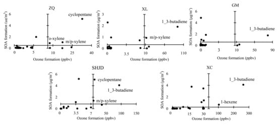
Figure 9.
The distribution of VOCs characterized by ozone and SOA formation.
5. Conclusions
The coupling of regional network observations was exploited to determine the effect of primary sources, namely the Complex and Second Industrial Zone, on the surrounding area. Four typical wind patterns were categorized for methodical VOCs pollution phenomena cognition, and LC and SE were the most common flows. Approximately 70% of the cases could be reasonably interpreted by wind flows, and high pollution events mostly arose under LC patterns. Ethylene and propylene emitted from petrochemical processes were precursors with the highest OFP values. Based on fingerprint profile investigations, ethylene (>3), ethylbenzene (>1), and T/B (<2) were chosen as indicators to distinguish contamination from the Complex, industrial area, and vehicular emissions. The TI% allowed evaluations of pollution extent at each site under the given wind pattern. It was found that the SW flow was related to the most serious pollution for GM, SHJD, and XC; and LC flow was related to that for ZQ and XL; GM suffered the most severe influence by the Complex, and XL was most affected by industrial processes. The good agreements with the profile analysis suggested the precision of the selection of indicators. The estimates of OH exposure, VOCs consumption, and ozone and SOA formation showed the magnitude of the photochemical reactions during transportation. XC under SW formed the most ozone, and GM under SE generated the least; SHJD produced the maximum amount of SOA, and XL produced the minimum. Emissions of cyclopentane, o-xylene, m/p-xylene, 1-3-butadiene, and 1-hexene should be reduced from the secondary formation point of view. This whole mechanism provided a qualitative and quantitative way to determine the influence of a governing source on a neighboring area, which can be widely applied with densely distributed stations.
Author Contributions
Conceptualization, K.L. and Y.L.; Methodology, Y.L. and W.Q.; Formal analysis, W.Q. and S.L.; Investigation, Y.L. and W.Q.; Resources, K.L.; Writing—original draft preparation, W.Q.; Writing—review and editing, K.L. and Y.L.; Project administration, K.L.; Funding acquisition, K.L.
Funding
This research was funded by the National Key Research and Development Plan (2017YFC0210004), and the National Natural Science Foundation of China (Grant No. 91544225).
Acknowledgments
This work was supported by the National Key Research and Development Plan (2017YFC0210004), the National Natural Science Foundation of China (Grant No. 91544225), and the study on the causes of ozone pollution in Shanghai (2016-12). The authors gratefully thank the science team of Peking University, as well as the team from Jinshan Environmental Monitor Station for their general support.
Conflicts of Interest
The authors declare no conflict of interest.
References
- Seinfeld, J.H.; Pandis, S.N. Atmospheric Chemistry and Physics; Wiley: Hoboken, NJ, USA, 2006. [Google Scholar]
- Pachauri, T.; Satsangi, A.; Singla, V.; Lakhani, A.; Kumari, K.M. Characteristics and Sources of Carbonaceous Aerosols in Pm2. 5 During Wintertime in Agra, India. Aerosol Air Qual. Res. 2013, 13, 977–991. [Google Scholar] [CrossRef]
- Poisson, N.; Kanakidou, M.; Crutzen, P.J. Impact of Non-Methane Hydrocarbons on Tropospheric Chemistry and the Oxidizing Power of the Global Troposphere: 3-Dimensional Modelling Results. J. Atmos. Chem. 2000, 36, 157–230. [Google Scholar] [CrossRef]
- Jobson, B.T.; Berkowitz, C.M.; Kuster, W.C.; Goldan, P.D.; Williams, E.J.; Fesenfeld, F.C.; Apel, E.C.; Karl, T.; Lonneman, W.A.; Riemer, D. Hydrocarbon Source Signatures in Houston, Texas: Influence of the Petrochemical Industry. J. Geophys. Res. Atmos. 2004, 109, D24. [Google Scholar] [CrossRef]
- Leuchner, M.; Rappenglück, B. Voc Source–Receptor Relationships in Houston During Texaqs-Ii. Atmos. Environ. 2010, 44, 4056–4067. [Google Scholar] [CrossRef]
- Ling, Z.H.; Guo, H. Contribution of Voc Sources to Photochemical Ozone Formation and Its Control Policy Implication in Hong Kong. Environ. Sci. Policy 2014, 38, 180–191. [Google Scholar] [CrossRef]
- Hou, X.; Strickland, M.J.; Liao, K.J. Contributions of Regional Air Pollutant Emissions to Ozone and Fine Particulate Matter-Related Mortalities in Eastern U.S. Urban Areas. Environ. Res. 2015, 137, 475–484. [Google Scholar] [CrossRef]
- Jiang, H.Y.; Li, H.R.; Yang, L.S.; Li, Y.H.; Wang, W.Y.; Yan, Y.C. Spatial and Seasonal Variations of the Air Pollution Index and a Driving Factors Analysis in China. J. Environ. Qual. 2014, 43, 1853–1863. [Google Scholar] [CrossRef]
- Zhang, X.; Zhao, W.; Meng, F. Study on Classification Control of Atmospheric Volatile Organic Compounds Emission Pollution Sources Based on Ofp. Environ. Prot. (Chinese version) 2017, 13, 23–26. [Google Scholar]
- Huang, C.; Chen, C.H.; Li, L.; Cheng, Z. Emission Inventory of Anthropogenic Air Pollutants and Voc Species in the Yangtze River Delta Region, China. Atmos. Chem. Phys. 2011, 11, 4105–4120. [Google Scholar] [CrossRef]
- Wang, H. Characterization of Volatile Organic Compounds (Vocs) and the Impact on Ozone Formation During the Photochemical Smog Episode in Shanghai, China. Acta Sci. Circumstantiae 2015, 35, 1603–1611. [Google Scholar]
- Wang, H.; Nie, L.; Li, J.; Wang, Y.; Wang, G.; Wang, J.; Hao, Z. Characterization and Assessment of Volatile Organic Compounds (Vocs) Emissions from Typical Industries. Chin. Sci. Bull. 2013, 58, 724–730. [Google Scholar] [CrossRef]
- Wu, W.; Zhao, B.; Wang, S.; Hao, J. Ozone and Secondary Organic Aerosol Formation Potential from Anthropogenic Volatile Organic Compounds Emissions in China. J. Environ. Sci. 2017, 53, 224–237. [Google Scholar] [CrossRef]
- Dumanoglu, Y.; Kara, M.; Altiok, H.; Odabasi, M.; Elbir, T.; Bayram, A. Spatial and Seasonal Variation and Source Apportionment of Volatile Organic Compounds (Vocs) in a Heavily Industrialized Region. Atmos. Environ. 2014, 98, 168–178. [Google Scholar] [CrossRef]
- Zhao, C.H.; Geng, F.H.; Ma, C.Y.; Chen, Y.H.; Mao, X.Q. Aerosol Characteristics During Photochemical Pollution in Shanghai Area. China Environ. Sci. 2015, 35, 356–363. [Google Scholar]
- Cheng, F.Y.; Chin, S.C.; Liu, T.H. The Role of Boundary Layer Schemes in Meteorological and Air Quality Simulations of the Taiwan Area. Atmos. Environ. 2012, 54, 714–727. [Google Scholar] [CrossRef]
- Angevine, W.M.; Senff, C.J.; White, A.B.; Williams, E.J.; Koermer, J.; Miller, S.T.; Talbot, R.; Johnston, P.E.; McKeen, S.A.; Downs, T. Coastal Boundary Layer Influence on Pollutant Transport in New England. J. Appl. Meteorol. 2004, 43, 1425–1437. [Google Scholar] [CrossRef]
- Chen, S.P.; Wang, C.H.; Lin, W.D.; Tong, Y.H.; Chen, Y.C.; Chiu, C.J.; Chiang, H.C.; Fan, C.L.; Wang, J.L.; Chang, J.S. Air Quality Impacted by Local Pollution Sources and Beyond - Using a Prominent Petro-Industrial Complex as a Study Case. Environ. Pollut. 2018, 236, 699–705. [Google Scholar] [CrossRef]
- Duan, J.; Tan, J.; Yang, L.; Wu, S.; Hao, J. Concentration, Sources and Ozone Formation Potential of Volatile Organic Compounds (Vocs) During Ozone Episode in Beijing. Atmos. Res. 2008, 88, 25–35. [Google Scholar] [CrossRef]
- Liu, Y.; Yuan, B.; Li, X.; Shao, M.; Lu, S.; Li, Y.; Chang, C.C.; Wang, Z.; Hu, W.; Huang, X.; et al. Impact of Pollution Controls in Beijing on Atmospheric Oxygenated Volatile Organic Compounds (Ovocs) During the 2008 Olympic Games: Observation and Modeling Implications. Atmos. Chem. Phys. 2015, 15, 3045–3062. [Google Scholar] [CrossRef]
- Cheng, H.; Guo, H.; Wang, X.; Saunders, S.M.; Lam, S.H.M.; Jiang, F.; Wang, T.; Ding, A.; Lee, S.; Ho, K.F. On the Relationship between Ozone and Its Precursors in the Pearl River Delta: Application of an Observation-Based Model (Obm). Environ. Sci. Pollut. Res. 2010, 17, 547–560. [Google Scholar] [CrossRef]
- Jin, X.; Holloway, T. Spatial and Temporal Variability of Ozone Sensitivity over China Observed from the Ozone Monitoring Instrument: Ozone Sensitivity over China. J. Geophys. Res. Atmos. 2015, 120, 7229–7246. [Google Scholar] [CrossRef]
- Kalabokas, P.D.; Hatzianestis, J.; Bartzis, J.G.; Papagiannakopoulos, P. Atmospheric Concentrations of Saturated and Aromatic Hydrocarbons around a Greek Oil Refinery. Atmos. Environ. 2001, 35, 2545–2555. [Google Scholar] [CrossRef]
- Brown, S.G.; Frankel, A.; Hafner, H.R. Source Apportionment of Vocs in the Los Angeles Area Using Positive Matrix Factorization. Atmos. Environ. 2007, 41, 227–237. [Google Scholar] [CrossRef]
- Liaud, C.; Nguyen, N.T.; Nasreddine, R.; le Calvé, S. Experimental Performances Study of a Transportable Gc-Pid and Two Thermo-Desorption Based Methods Coupled to Fid and Ms Detection to Assess Btex Exposure at Sub-Ppb Level in Air. Talanta 2014, 127, 33–42. [Google Scholar] [CrossRef]
- Nasreddine, R.; Person, V.; Serra, C.A.; le Calvé, S. Development of a Novel Portable Miniaturized Gc for near Real-Time Low Level Detection of Btex. Sens. Actuators B Chem. 2016, 224, 159–169. [Google Scholar] [CrossRef]
- Cai, X.M.; Steyn, D.G. Modelling Study of Sea Breezes in a Complex Coastal Environment. Atmos. Environ. 2000, 34, 2873–2885. [Google Scholar] [CrossRef]
- Levy, I.; Mahrer, Y.; Dayan, U. Coastal and Synoptic Recirculation Affecting Air Pollutants Dispersion: A Numerical Study. Atmos. Environ. 2009, 43, 1991–1999. [Google Scholar] [CrossRef]
- Su, Y.C.; Chen, S.P.; Tong, Y.H.; Fan, C.L.; Chen, W.H.; Wang, J.L.; Chang, J.S. Assessment of Regional Influence from a Petrochemical Complex by Modeling and Fingerprint Analysis of Volatile Organic Compounds (Vocs). Atmos. Environ. 2016, 141, 394–407. [Google Scholar] [CrossRef]
- Jia, C.; Batterman, S.; Godwin, C. Vocs in Industrial, Urban and Suburban Neighborhoods, Part 1: Indoor and Outdoor Concentrations, Variation, and Risk Drivers. Atmos. Environ. 2008, 42, 2083–2100. [Google Scholar] [CrossRef]
- Prinn, R.; Cunnold, D.; Rasmussen, R.; Simmonds, P.; Alyea, F.; Crawford, A.; Fraser, P.; Rosen, R. Atmospheric Trends in Methylchloroform and the Global Average for the Hydroxyl Radical. Science 1987, 238, 945–950. [Google Scholar] [CrossRef]
- Liu, P.W.G.; Yao, Y.C.; Tsai, J.H.; Hsu, Y.C.; Chang, L.P.; Chang, K.H. Source Impacts by Volatile Organic Compounds in an Industrial City of Southern Taiwan. Sci. Total Environ. 2008, 398, 154–163. [Google Scholar] [CrossRef]
- Cai, C.; Geng, F.; Tie, X.; Yu, Q.; An, J. Characteristics and Source Apportionment of Vocs Measured in Shanghai, China. Atmos. Environ. 2010, 44, 5005–5014. [Google Scholar] [CrossRef]
- Wang, G.; Cheng, S.; Wei, W.; Zhou, Y.; Yao, S.; Zhang, H. Characteristics and Source Apportionment of Vocs in the Suburban Area of Beijing, China. Atmos. Pollut. Res. 2016, 7, 711–724. [Google Scholar] [CrossRef]
- Gong, Y.; Wei, Y.; Cheng, J.; Jiang, T.; Chen, L.; Xu, B. Health Risk Assessment and Personal Exposure to Volatile Organic Compounds (Vocs) in Metro Carriages—a Case Study in Shanghai, China. Sci. Total Environ. 2017, 574, 1432–1438. [Google Scholar] [CrossRef]
- Scheff, P.A.; Wadden, R.A.; Bates, B.A.; Aronian, P.F. Source Fingerprints for Receptor Modeling of Volatile Organics. Japca 1989, 39, 469–478. [Google Scholar] [CrossRef]
- Liu, Y.; Shao, M.; Fu, L.; Lu, S.; Zeng, L.; Tang, D. Source Profiles of Volatile Organic Compounds (Vocs) Measured in China: Part I. Atmos. Environ. 2008, 42, 6247–6260. [Google Scholar] [CrossRef]
- Osadetz, K.G.; Brooks, P.W.; Snowdon, L.R. Oil Families and Their Sources in Canadian Williston Basin, (Southeastern Saskatchewan and Southwestern Manitoba). Bull. Can. Pet. Geol. 1992, 40, 254–273. [Google Scholar]
- Wang, H.; Qiao, Y.; Chen, C.; Lu, J.; Dai, H.X.; Qiao, L.P.; Lou, S.; Huang, C.; Jing, S.; Wu, J.P. Source Profiles and Chemical Reactivity of Volatile Organic Compounds from Solvent Use in Shanghai, China. Aerosol Air Qual. Res. 2014, 14, 301–310. [Google Scholar] [CrossRef]
- Sexton, K.; Westberg, H. Photochemical Ozone Formation from Petroleum Refinery Emissions. Atmos. Environ. (1967) 1983, 17, 467–475. [Google Scholar] [CrossRef]
- Na, K.; Moon, K.C.; Kim, Y.P. Source Contribution to Aromatic Voc Concentration and Ozone Formation Potential in the Atmosphere of Seoul. Atmos. Environ. 2005, 39, 5517–5524. [Google Scholar] [CrossRef]
- Zhu, S.; Huang, X.; He, L.; Lu, S.; Feng, N. Variation Characteristics and Chemical Reactivity of Ambient Vocs in Shenzhen. China Environ. Sci. 2012, 32, 2140–2148. [Google Scholar]
- Gao, Z.; Gao, S.; Cui, H.; Fu, Q.; Jin, D.; Liang, G.; Fang, F. Characteristics and Chemical Reactivity of Vocs During a Typical Photochemical Episode in Summer at a Chemical Industrial Area. Acta Sci. Circumstantiae 2017, 4, 5. [Google Scholar]
- Atkinson, R.; Arey, J. Atmospheric Degradation of Volatile Organic Compounds. Chem. Rev. 2003, 103, 4605–4638. [Google Scholar] [CrossRef]
- Laowagul, W.; Yoshizumi, K. Behavior of Benzene and 1,3-Butadiene Concentrations in the Urban Atmosphere of Tokyo, Japan. Atmos. Environ. 2009, 43, 2052–2059. [Google Scholar] [CrossRef]
- Carter, W.P.L. Saprc Atmospheric Chemical Mechanisms and Voc Reactivity Scales. Available online: www.cert.ucr.edu/~carter/SAPRC (accessed on 18 October 2019).
- Fenske, J.D.; Hasson, A.S.; Ho, A.W.; Paulson, S.E. Measurement of Absolute Unimolecular and Bimolecular Rate Constants for Ch 3 Choo Generated by the Trans -2butene Reaction with Ozone in the Gas Phase. J. Phys. Chem. A 2000, 104, 9921–9932. [Google Scholar] [CrossRef]
- Cui, H.X.; Wu, Y.M.; Gao, S.; Duan, Y.S.; Wang, D.F.; Zhang, Y.H.; Fu, Q.Y. Characteristics of Ambient Vocs and Their Role in O3 Formation: A Typical Air Pollution Episode in Shanghai Urban Area. Huan Jing Ke Xue 2011, 32, 3537–3542. [Google Scholar]
- Geng, F.; Zhao, C.; Tang, X.; Lu, G.; Tie, X. Analysis of Ozone and Vocs Measured in Shanghai: A Case Study. Atmos. Environ. 2007, 41, 989–1001. [Google Scholar] [CrossRef]
- Geng, F.; Zhang, Q.; Tie, X.; Huang, M.; Ma, X.; Deng, Z.; Yu, Q.; Quan, J.; Zhao, C. Aircraft Measurements of O3, Nox, Co, Vocs, and So2 in the Yangtze River Delta Region. Atmos. Environ. 2009, 43, 584–593. [Google Scholar] [CrossRef]
- An, J.; Zhu, B.; Wang, H.; Li, Y.; Lin, X.; Yang, H. Characteristics and Source Apportionment of Vocs Measured in an Industrial Area of Nanjing, Yangtze River Delta, China. Atmos. Environ. 2014, 97, 206–214. [Google Scholar] [CrossRef]
- Guo, H.; Wang, T.; Simpson, I.J.; Blake, D.R.; Yu, X.M.; Kwok, Y.H.; Li, Y.S. Source Contributions to Ambient Vocs and Co at a Rural Site in Eastern China. Atmos. Environ. 2004, 38, 4551–4560. [Google Scholar] [CrossRef]
- Tang, J.H.; Chan, L.Y.; Chan, C.Y.; Li, Y.S.; Chang, C.C.; Liu, S.C.; Wu, D.; Li, Y.D. Characteristics and Diurnal Variations of Nmhcs at Urban, Suburban, and Rural Sites in the Pearl River Delta and a Remote Site in South China. Atmos. Environ. 2007, 41, 8620–8632. [Google Scholar] [CrossRef]
- Chen, C.H.; Su, L.Y.; Wang, H.L.; Huang, C.; Li, L.; Zhou, M.; Qiao, Y.; Chen, Y.; Chen, M.; Huang, H.; et al. Variation and Key Reactive Species of Ambient Vocs in the Urban Area of Shanghai, China. Acta Sci. Circumst. 2012, 32, 367–376. [Google Scholar]
- Chang, C.C.; Wang, J.L.; Lung, S.C.C.; Liu, S.C.; Shiu, C.J. Source Characterization of Ozone Precursors by Complementary Approaches of Vehicular Indicator and Principal Component Analysis. Atmos. Environ. 2009, 43, 1771–1778. [Google Scholar] [CrossRef]
- Zhang, Y.; Wang, X.; Barletta, B.; Simpson, I.J.; Blake, D.R.; Fu, X.; Zhang, Z.; He, Q.; Liu, T.; Zhao, X.; et al. Source Attributions of Hazardous Aromatic Hydrocarbons in Urban, Suburban and Rural Areas in the Pearl River Delta (Prd) Region. J. Hazard. Mater. 2013, 250, 403–411. [Google Scholar] [CrossRef] [PubMed]
- Zhang, L.; Zhu, B.; Gao, J.H.; Kang, H.Q.; Yang, P.; Wang, H.L.; Ye, L.; Shao, P. Modeling Study of a Typical Summer Ozone Pollution Event over Yangtze River Delta. Huan Jing Ke Xue 2015, 36, 3981–3988. [Google Scholar] [PubMed]
- Atkinson, R.; Carter, W.P.L.; Winer, A.M.; Pitts, J.N., Jr. An Experimental Protocol for the Determination of Oh Radical Rate Constants with Organics Using Methyl Nitrite Photolysis as an Oh Radical. J. Air Pollut. Control Assoc. 1981, 31, 1090–1092. [Google Scholar] [CrossRef][Green Version]
- Shilling, J.E.; Chen, Q.; King, S.M.; Rosenoern, T.; Kroll, J.H.; Worsnop, D.R.; McKinney, K.A.; Martin, S.T. Particle Mass Yield in Secondary Organic Aerosol Formed by the Dark Ozonolysis of A-Pinene. Atmos. Chem. Phys. 2008, 8, 2073–2088. [Google Scholar] [CrossRef]
- Yuan, B.; Hu, W.W.; Shao, M.; Wang, M.; Chen, W.T.; Lu, S.H.; Zeng, L.M.; Hu, M. Voc Emissions, Evolutions and Contributions to Soa Formation at a Receptor Site in Eastern China. Atmos. Chem. Phys. 2013, 13, 8815–8832. [Google Scholar] [CrossRef]
- Blake, N.J.; Penkett, S.A.; Clemitshaw, K.C.; Anwyl, P.; Lightman, P.; Marsh, A.R.W.; Butcher, G. Estimates of Atmospheric Hydroxyl Radical Concentrations from the Observed Decay of Many Reactive Hydrocarbons in Well-Defined Urban Plumes. J. Geophys. Res.-Atmos. 1993, 98, 2851–2864. [Google Scholar] [CrossRef]
- Kleinman, L.I.; Daum, P.H.; Lee, Y.N.; Nunnermacker, L.J.; Springston, S.R.; Weinstein-Lloyd, J.; Hyde, P.; Doskey, P.; Rudolph, J.; Fast, J.; et al. Photochemical Age Determinations in the Phoenix Metropolitan Area. J. Geophys. Res.-Atmos. 2003, 108, D3. [Google Scholar] [CrossRef]
- Sun, J.; Wu, F.; Hu, B.; Tang, G.; Zhang, J.; Wang, Y. Voc Characteristics, Emissions and Contributions to Soa Formation During Hazy Episodes. Atmos. Environ. 2016, 141, 560–570. [Google Scholar] [CrossRef]
- Atkinson, R.; Baulch, D.L.; Cox, R.A.; Crowley, J.N.; Hampson, R.F.; Hynes, R.G.; Jenkin, M.E.; Rossi, M.J.; Troe, J.; Subcommittee, I.U.P.A.C. Evaluated Kinetic and Photochemical Data for Atmospheric Chemistry: Volume Ii–Gas Phase Reactions of Organic Species. Atmos. Chem. Phys. 2006, 6, 3625–4055. [Google Scholar] [CrossRef]
- Jacob, D.J. Introduction to Atmospheric Chemistry; Princeton, N.J., Ed.; Princeton University Press: Princeton, NJ, USA, 1999. [Google Scholar]
- Derwent, R.G.; Jenkin, M.E.; Utembe, S.R.; Shallcross, D.E.; Murrells, T.P.; Passant, N.R. Secondary Organic Aerosol Formation from a Large Number of Reactive Man-Made Organic Compounds. Sci. Total Environ. 2010, 408, 3374–3381. [Google Scholar] [CrossRef] [PubMed]
© 2019 by the authors. Licensee MDPI, Basel, Switzerland. This article is an open access article distributed under the terms and conditions of the Creative Commons Attribution (CC BY) license (http://creativecommons.org/licenses/by/4.0/).