Response of Near-Surface Meteorological Conditions to Advection under Impact of the Green Roof


Abstract
1. Introduction
2. Methodology
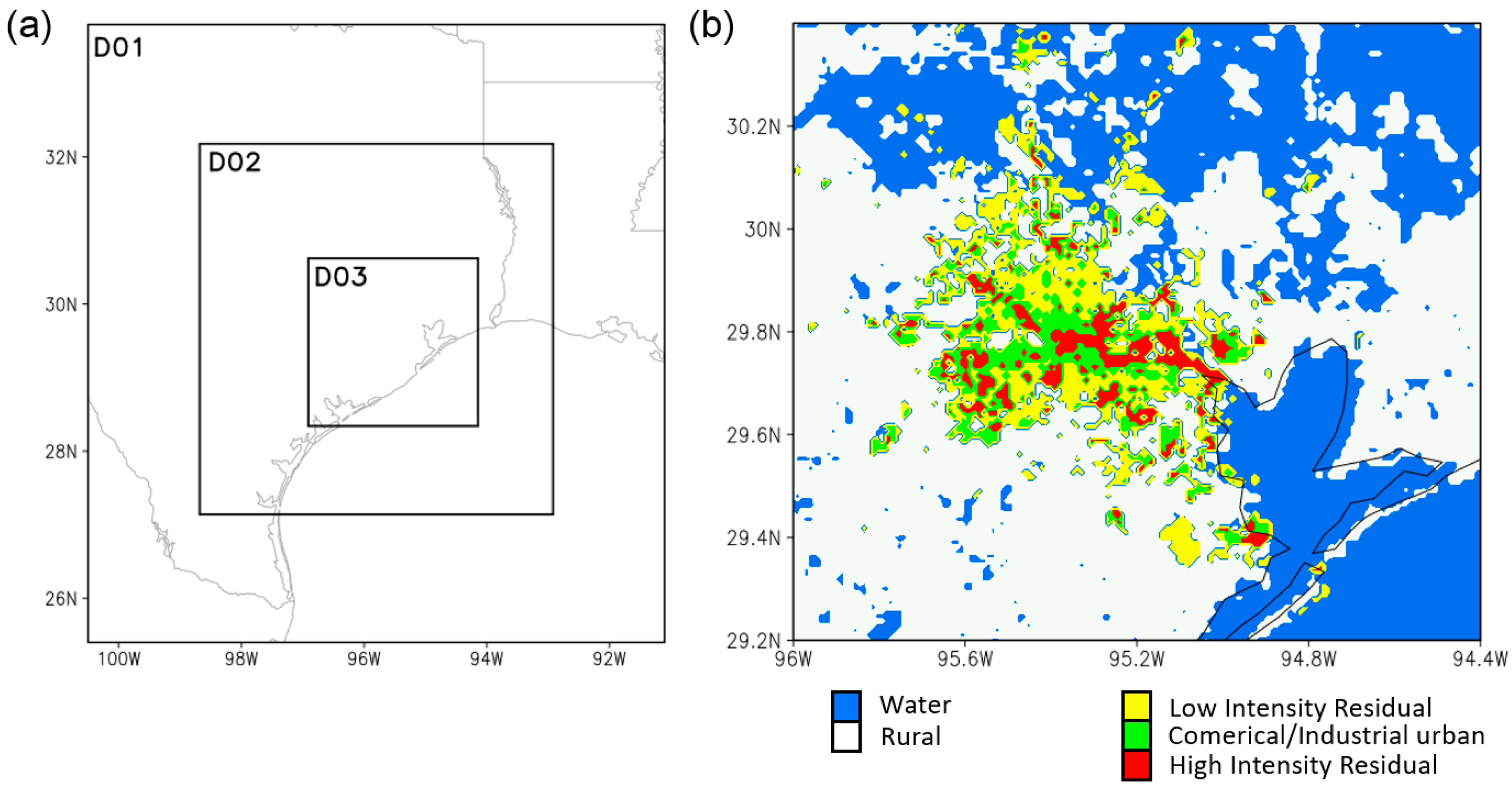
2.1. Model
2.2. Simulations
2.3. Data and Method
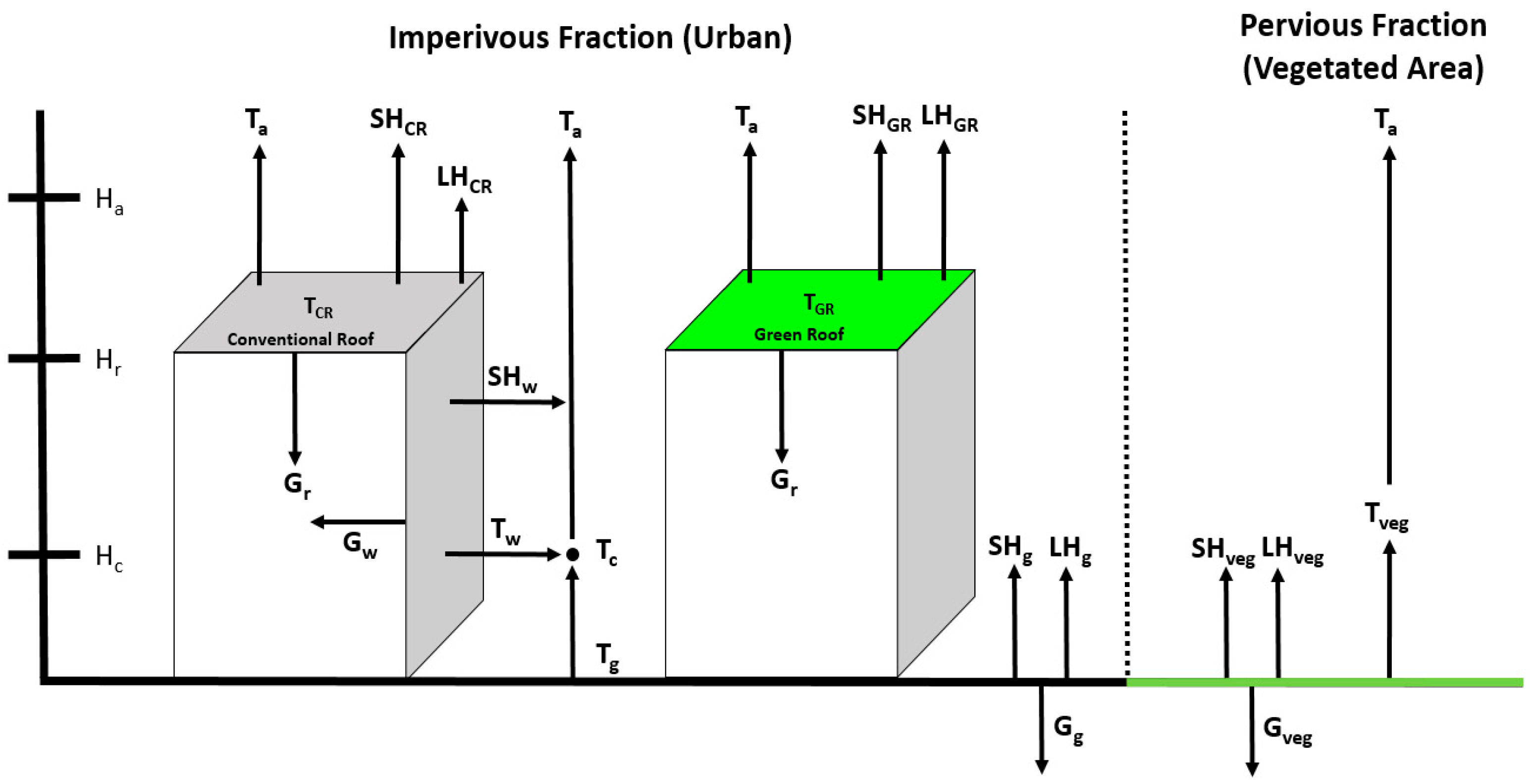
2.4. Green Roof Modeling
3. Results
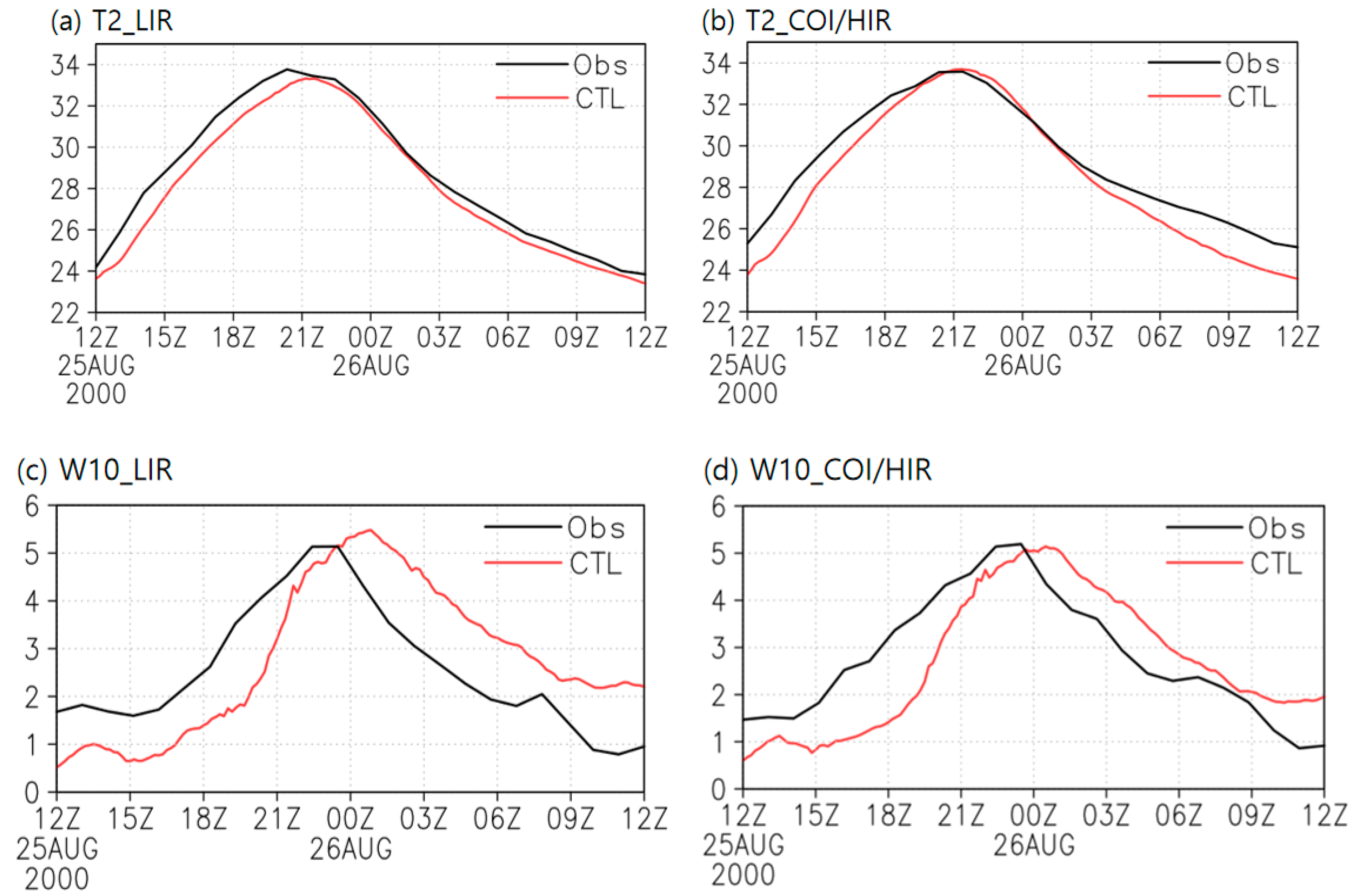
3.1. Near-Surface Temperature and Winds
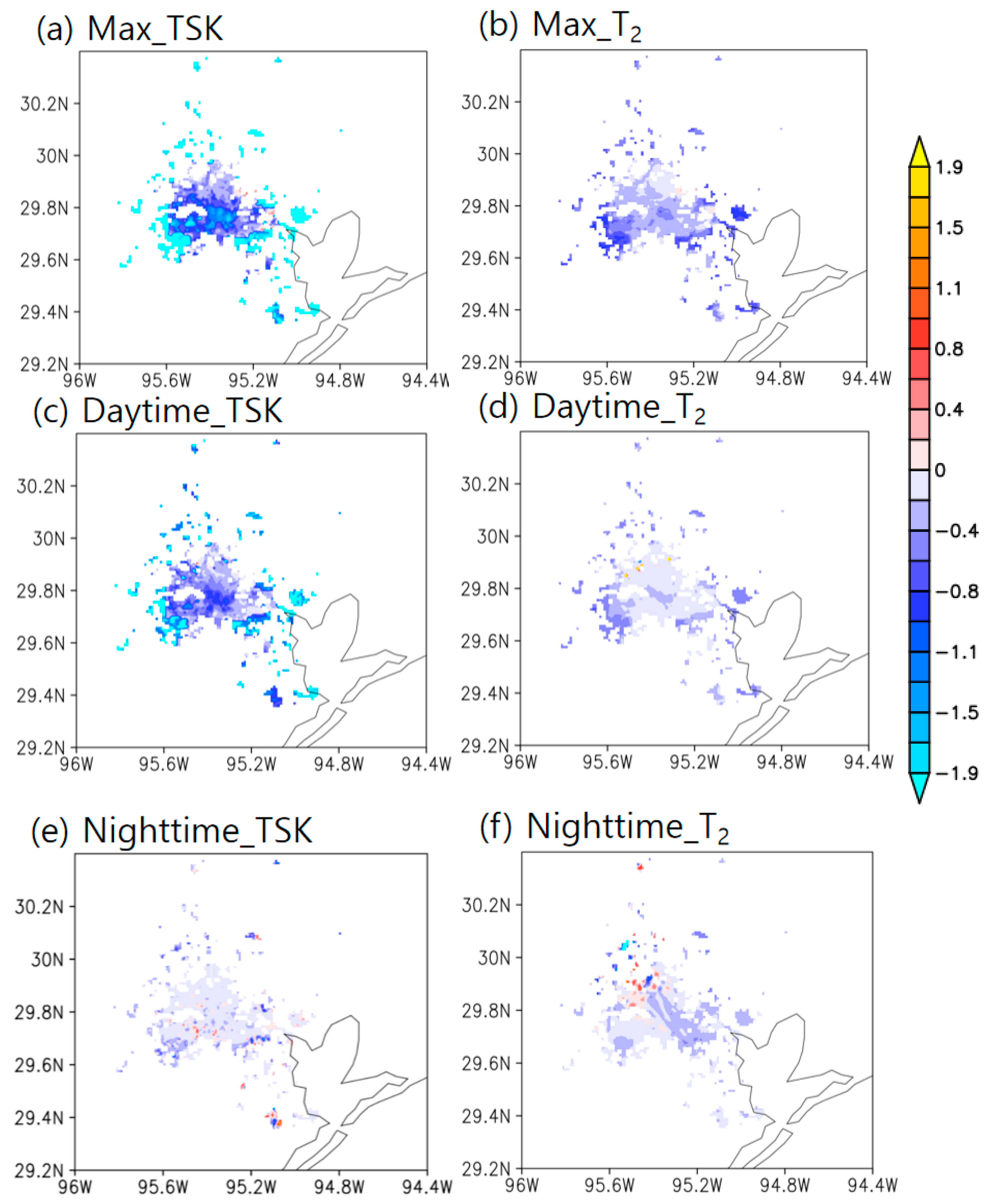
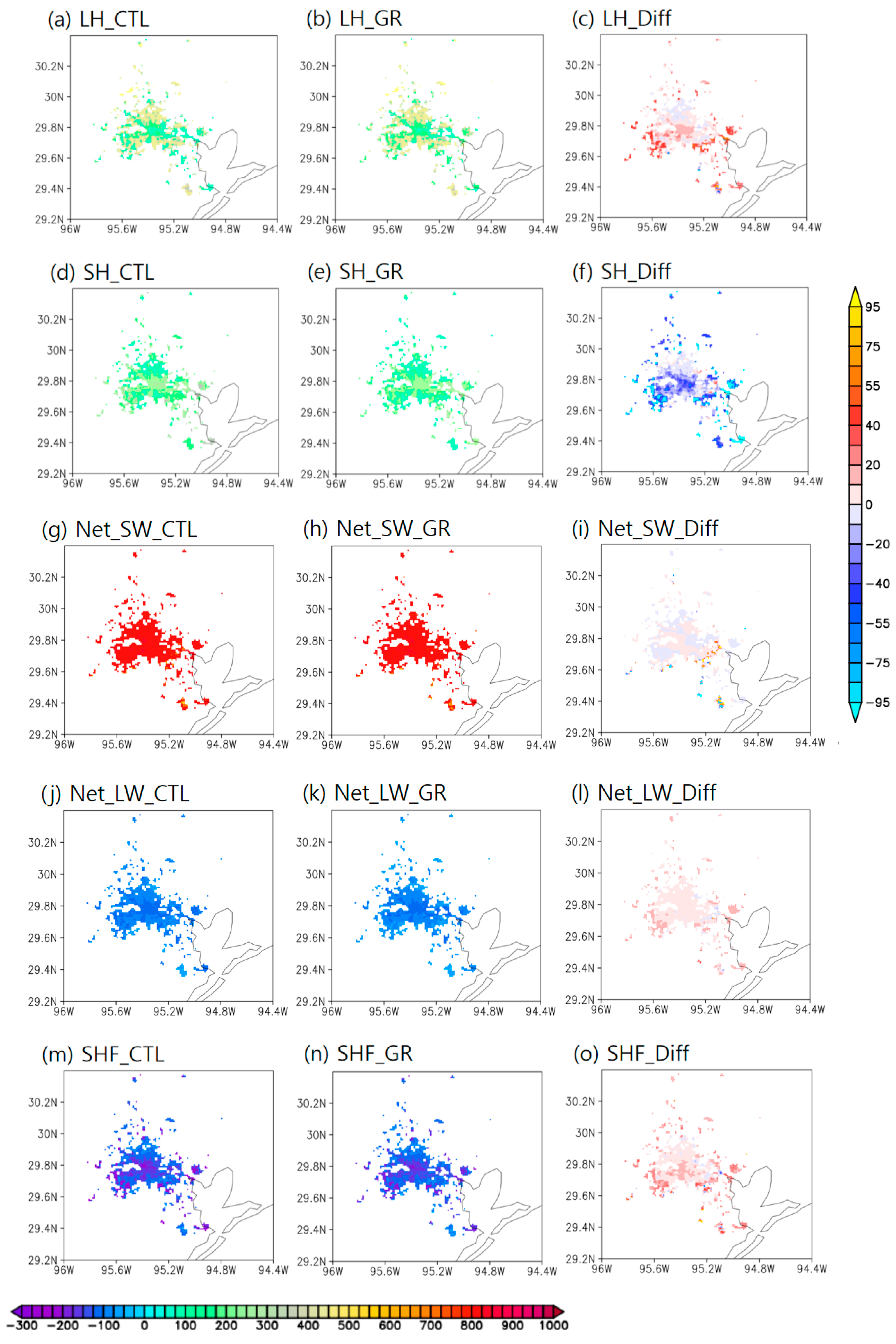
3.2. Surface Heat Flux
3.3. Role of Advection
3.3.1. Temperature Advection
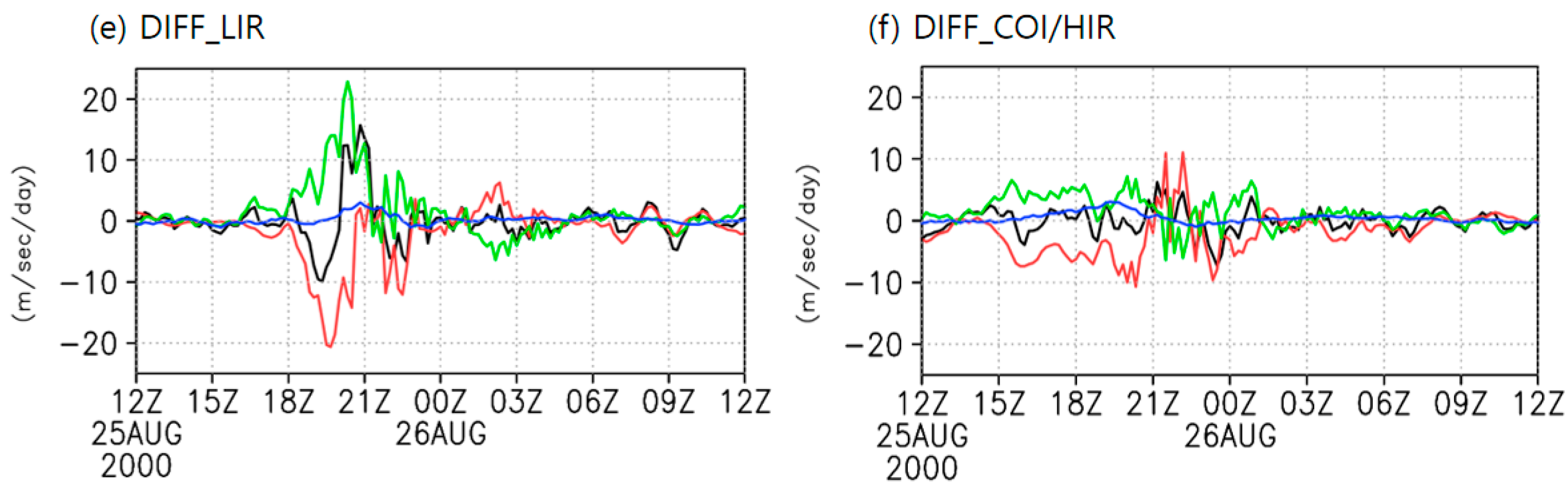
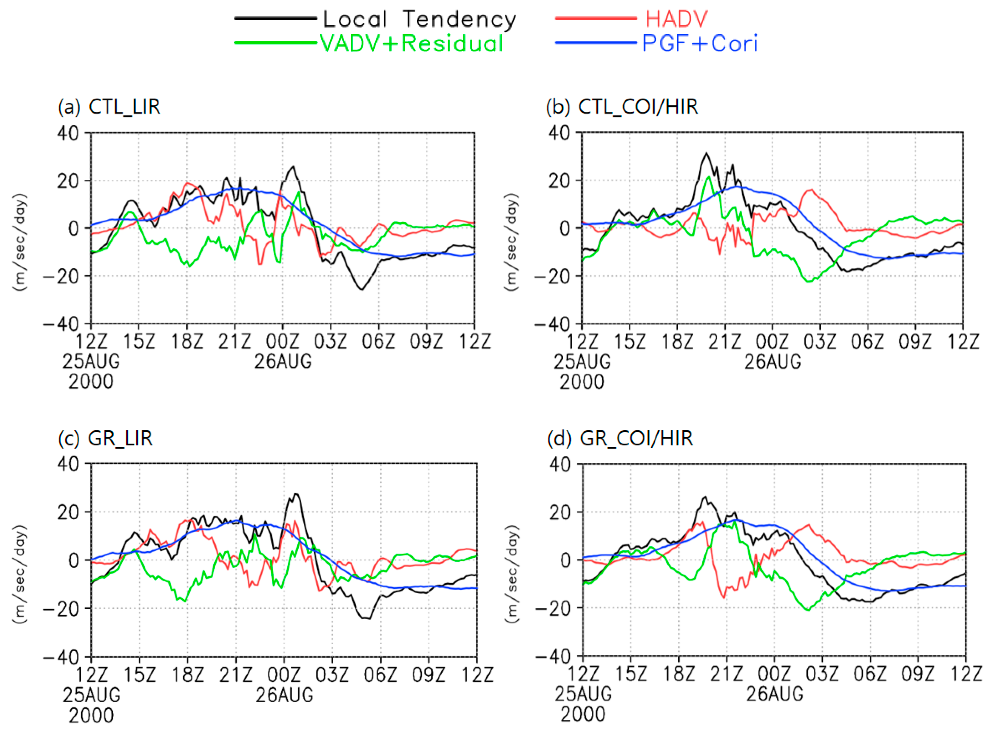
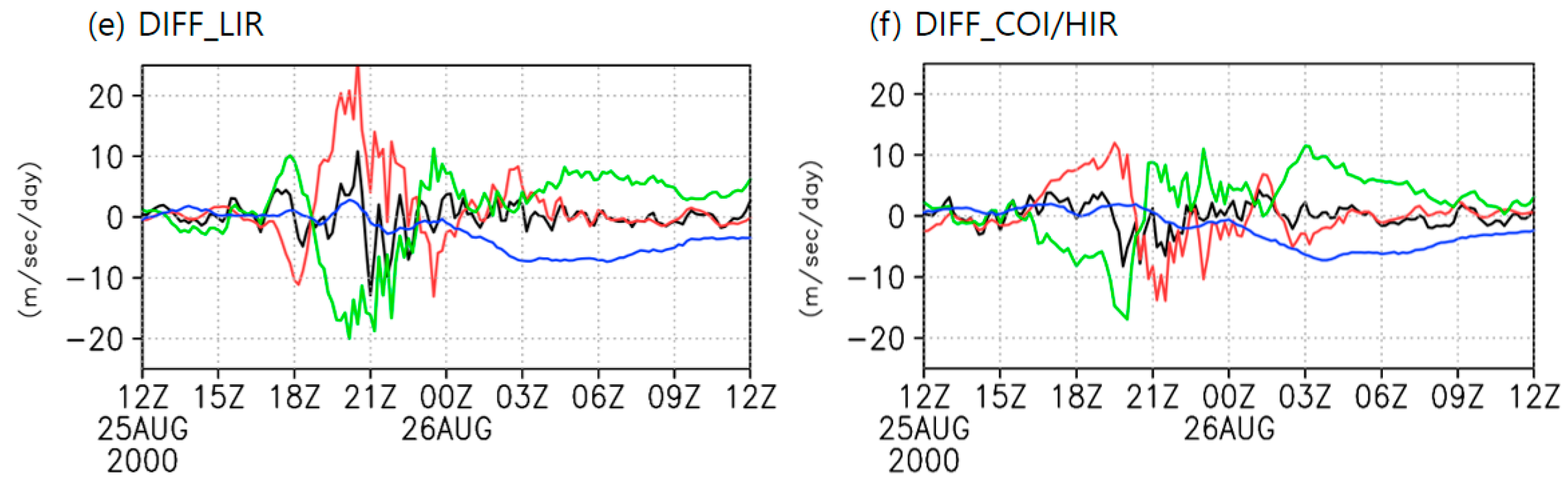
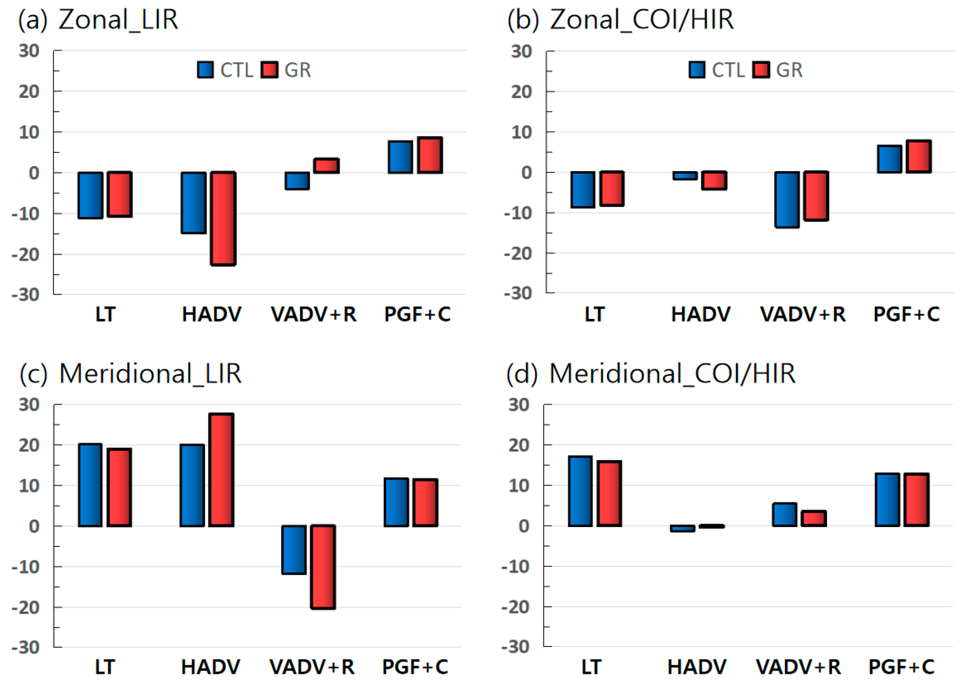
3.3.2. Momentum Advection
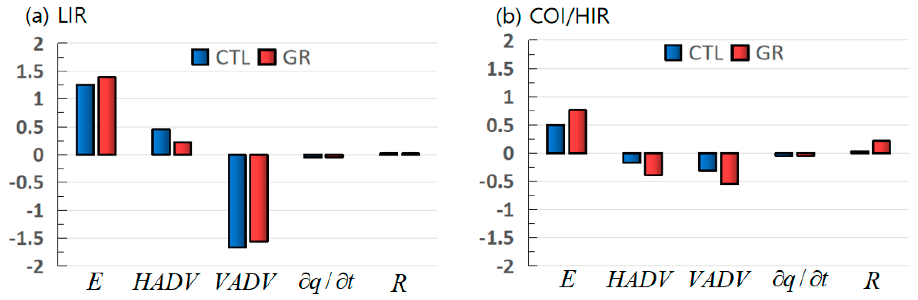
3.3.3. Moisture Advection
4. Discussion
5. Conclusions
Author Contributions
Funding
Acknowledgments
Conflicts of Interest
References
- Seto, K.C.; Fragkias, M.; Guneralp, B.; Reilly, M.K. A meta-analysis of global urban land expansion. PLoS ONE 2011, 6, e23777. [Google Scholar] [CrossRef] [PubMed]
- Arnfield, A.J. Two decades of urban climate research: A review of turbulence, exchanges of energy and water, and the urban heat island. Int. J. Climatol. 2003, 23, 1–26. [Google Scholar] [CrossRef]
- Yang, J.; Wang, Z.H.; Chen, F.; Miao, S.; Tewari, M.; Voogt, J.; Myint, S. Enhancing hydrologic modelling in the coupled Weather Research and Forecasting-urban modelling system. Bound. Layer Meteorol. 2015, 155, 87–109. [Google Scholar] [CrossRef]
- Burian, S.J.; Shepherd, J.M. Effect of urbanization on the diurnal rainfall pattern in Houston. Hydrol. Process. 2005, 19, 1089–1103. [Google Scholar] [CrossRef]
- Oleson, K.W.; Bonan, G.B.; Feddema, J.; Jackson, T. An examination of urban heat island characteristics in a global climate model. Int. J. Climatol. 2011, 31, 1848–1865. [Google Scholar] [CrossRef]
- Unkasevic, M.; Jovanovic, O.; Popovic, T. Urban-suburban/rural vapour pressure and relative humidity differences at fixed hours over the area of Belgrade city. Theor. Appl. Climatol. 2001, 68, 67–73. [Google Scholar] [CrossRef]
- Georgescu, M.; Mahalov, A.; Moustaoui, M. Seasonal hydroclimatic impacts of Sun Corridor expansion. Environ. Res. Lett. 2012, 7, 034026. [Google Scholar] [CrossRef]
- Bornstein, R.D.; Johnson, D.S. Urban-rural wind velocity differences. Atmos. Environ. 1977, 11, 597–604. [Google Scholar] [CrossRef]
- Fernando, H.J.S. Fluid dynamics of urban atmospheres in complex terrain. Annu. Rev. Fluid Mech. 2010, 42, 365–389. [Google Scholar] [CrossRef]
- Landsberg, H.E. The Urban Climate; Academic Press: New York, NY, USA, 1981; 275p. [Google Scholar]
- Oke, T.R. The energetic basis of the urban heat island. Q. J. R. Meteorol. Soc. 1982, 108, 1–24. [Google Scholar] [CrossRef]
- Hassid, S.; Santamouris, M.; Papanikolaou, N.; Linardi, A.; Klitsikas, N.; Georgakis, C.; Assimakopoulos, D.N. The effect of the Athens heat island on air conditioning load. Energy Build. 2000, 32, 131–141. [Google Scholar] [CrossRef]
- Cartalis, C.; Synodinou, A.; Proedrou, M.; Tsangrasoulis, A.; Santamouris, M. Modification in energy demand in urban areas as a result of climate changes: An assessment for the Southeast Mediterranean region. Energy Convers. Manag. 2001, 42, 1647–1656. [Google Scholar] [CrossRef]
- Santamouris, M.; Papanikolaou, N.; Livada, I.; Koronakis, I.; Georgakis, C.; Argiriou, A.; Assimakopoulos, D.N. On the impact of urban climate to the energy consumption of buildings. Sol. Energy 2001, 70, 201–216. [Google Scholar] [CrossRef]
- Grimmond, S. Urbanization and global environmental change: Local effects of urban warming. Cities Glob. Environ. Chang. 2007, 173, 83–88. [Google Scholar] [CrossRef]
- Rosenfeld, A.H.; Akbari, H.; Bretz, S.; Fishman, B.L.; Kurn, D.M.; Sailor, D.; Taha, H. Mitigation of urban heat islands: Material, utility programs, updates. Energy Build. 1995, 22, 255–265. [Google Scholar] [CrossRef]
- Akbari, H.; Pomerantz, M.; Taha, H. Cool surfaces and shade trees to reduce energy use and improve air quality in urban areas. Sol. Energy 2001, 70, 295–310. [Google Scholar] [CrossRef]
- Akbari, H.; Levinson, R. Evolution of cool-roof standards in the U.S. Adv. Build. Energy Res. 2008, 2, 1–32. [Google Scholar] [CrossRef]
- Theodosiou, T. Green roofs in buildings: Thermal and environmental behavior. Adv. Build. Energy Res. 2009, 3, 271–288. [Google Scholar] [CrossRef]
- Sfakianaki, A.; Pagalou, E.; Pavlou, K.; Santamouris, M.; Assimakopoulos, M. Theoretical and experimental analysis of the thermal behavior of a green roof system installed in two residential buildings in Athens, Greece. Int. J. Energy Res. 2009, 33, 1059–1069. [Google Scholar] [CrossRef]
- Zinzi, M. Cool materials and cool roofs: Potentialities in Mediterranean buildings. Adv. Build. Energy Res. 2010, 4, 201–266. [Google Scholar] [CrossRef]
- Gaitani, N.; Spanou, A.; Saliari, M.; Synnefa, A.; Vassilakopoulou, K.; Papadopoulou, K.; Pavlou, K.; Santamouris, M.; Papaioannou, M.; Lagoudaki, A. Improving the microclimate in urban areas: A case study in the centre of Athens. J. Build. Serv. Eng. 2011, 32, 53–71. [Google Scholar] [CrossRef]
- Chow, W.T.L.; Chuang, W.C.; Gober, P. Vulnerability to extreme heat in metropolitan Phoenix: Spatial, temporal, and demographic dimensions. Prof. Geogr. 2012, 64, 286–302. [Google Scholar] [CrossRef]
- Takebayashi, H.; Moriyama, M. Study of a simple evaluation method of urban heat island mitigation technology using upper-air data. J. Heat Isl. Inst. Int. 2012, 7, 102–110. [Google Scholar]
- Santamouris, M. On the energy impact of urban heat island and global warming on buildings. Energy Build. 2014, 82, 100–113. [Google Scholar] [CrossRef]
- Akbari, H.; Rose, L.S. Urban surfaces and heat island mitigation potential. J. Hum. Environ. Syst. 2007, 11, 85–101. [Google Scholar] [CrossRef]
- Georgescu, M. Challenges associated with adaptation to future urban expansion. J. Clim. 2015, 28, 2544–2563. [Google Scholar] [CrossRef]
- Yang, J.; Yu, Q.; Gong, P. Quantifying air pollution removal by green roofs in Chicago. Atmos. Environ. 2008, 42, 7266–7273. [Google Scholar] [CrossRef]
- Skamarock, W.C.; Klemp, J.B.; Dudhia, J.; Gill, D.O.; Barker, D.M.; Duda, M.G.; Huang, X.-Y.; Wang, W.; Powers, J.G. A Description of the Advanced Research WRF Version 3. NCAR Technical Note NCAR/TN-475+STR. NCAR Tech. Notes 2008. [Google Scholar] [CrossRef]
- Kusaka, H.; Kondo, H.; Kikegawa, Y.; Kimura, F. A simple single-layer urban canopy model for atmospheric models: Comparison with multilayer and slab models. Bound. Layer Meteorol. 2001, 101, 329–358. [Google Scholar] [CrossRef]
- Wang, Z.H.; Bou-Zeid, E.; Au, S.K.; Smith, J.A. Analyzing the sensitivity of WRF’s single-layer urban canopy model to parameter uncertainty using advanced Monte Carlo simulation. J. Appl. Meteorol. Climatol. 2011, 50, 1795–1814. [Google Scholar] [CrossRef]
- Wang, Z.H.; Smith, J.A. A spatially-analytical scheme for surface temperatures and conductive heat fluxes in urban canopy models. Bound. Layer Meteorol. 2011, 138, 171–193. [Google Scholar] [CrossRef]
- Grimmond, C.S.B.; Blacketta, M.; Bestb, M.J.; Barlowc, J.; Baikd, J.-J.; Belcherc, S.E.; Bohnenstengelc, S.I.; Calmete, I.; Chenf, F.; Dandoug, A.; et al. The International Urban Energy Balance Models Comparison Project: First results from phase 1. J. Appl. Meteorol. Climatol. 2010, 49, 1268–1292. [Google Scholar] [CrossRef]
- Lee, S.H.; Kim, S.W.; Angevine, W.M.; Bianco, L.; McKeen, S.A.; Senff, C.J.; Trainer, M.; Tucker, S.C.; Zamora, R.J. Evaluation of urban surface parameterization in WRF model using measurements during the Texas Air Quality Study 2006 field campaign. Atmos. Chem. Phys. 2011, 11, 2127–2143. [Google Scholar] [CrossRef]
- Wang, Z.H.; Bou-Zeid, E.; Smith, J.A. A coupled energy transport and hydrological model for urban canopies evaluated using a wireless sensor network. Q. J. Meteorol. Soc. 2013, 139, 1643–1657. [Google Scholar] [CrossRef]
- Miao, S.; Chen, F. Formation of horizontal convective rolls in urban areas. Atmos. Res. 2008, 89, 298–304. [Google Scholar] [CrossRef]
- Brownlee, J.; Ray, P.; Tewari, M.; Tan, H. Relative role of turbulent and radiative flux on the near-surface temperature in a single-layer urban canopy model over Houston. J. Appl. Meteorol. Climatol. 2017, 56, 2173–2187. [Google Scholar] [CrossRef]
- Li, D.; Bou-Zeid, E. Synergistic interactions between urban heat islands and heat waves: The impact in cities is larger than the sum of its parts. J. Appl. Meteorol. Climatol. 2013, 52, 2051–2064. [Google Scholar] [CrossRef]
- Streutker, D.R. Satellite-measured growth of the urban heat island of Houston, Texas. Remote Sens. Environ. 2003, 85, 282–289. [Google Scholar] [CrossRef]
- Salamanca, F.; Martilli, A.; Tewari, M.; Chen, F. A study of the urban boundary layer using different urban parameterizations and high-resolution urban canopy parameters with WRF. J. Appl. Meteorol. Climatol. 2011, 50, 1107–1128. [Google Scholar] [CrossRef]
- Smith, K.R.; Roebber, P. Green roof mitigation potential for a proxy future climate scenario in Chicago, Illinois. J. Appl. Meteorol. Climatol. 2011, 50, 507–522. [Google Scholar] [CrossRef]
- Sun, T.; Grimmond, C.S.B.; Ni, G.H. How do green roofs mitigate urban thermal stress under heat waves? J. Geophy. Res. Atmos. 2016, 121, 5320–5335. [Google Scholar] [CrossRef]
- Yang, J.; Wang, Z.H.; Georgescu, M.; Chen, F.; Tewari, M. Assessing the impact of enhanced hydrological processes on urban hydrometeorology with application to two cities in contrasting climates. J. Hydrometeorol. 2016, 17, 1031–1047. [Google Scholar] [CrossRef]
- Sharma, A.; Conry, P.; Fernando, H.J.S.; Hamlet, A.F.; Hellmann, J.J.; Chen, F. Green and cool roofs to mitigate urban heat island effects in the Chicago metropolitan area: Evaluation with a regional climate model. Environ. Res. Lett. 2016, 11, 064004. [Google Scholar] [CrossRef]
- Tewari, M.; Yang, J.; Kusaka, H.; Salamanca, F.; Watson, C.; Treinish, L. Interaction of urban heat islands and heat waves under current and future climate conditions and their mitigation using green and cool roofs in New York City and Phoenix, Arizona. Environ. Res. Lett. 2019, 14, 034002. [Google Scholar] [CrossRef]
- De Munck, C.; Lemonsu, A.; Bouzouidja, R.; Masson, V.; Claverie, R. The GREENROOF module (v7.3) for modelling green roof hydrological and performances within TED. Geosci. Model Dev. 2013, 6, 1941–1960. [Google Scholar] [CrossRef]
- Xie, X.M.; Nielsen-Gammon, J.W.; Zhang, F. Evaluation of three planetary boundary layer schemes in the WRF model. J. Appl. Meteorol. Climatol. 2010, 49, 1831–1844. [Google Scholar]
- Xie, B.; Fung, J.C.H.; Chan, A.; Lau, A. Evaluation of nonlocal and local planetary boundary layer schemes in the WRF model. J. Geophys. Res. 2012, 117, D12103. [Google Scholar] [CrossRef]
- Cohen, A.E.; Cavallo, S.M.; Coniglio, M.C.; Brooks, H.E. A review of planetary boundary layer parameterization schemes and their sensitivity in simulating southeastern U.S. cold season severe weather environments. Weather Forecast. 2015, 30, 591–612. [Google Scholar] [CrossRef]
- Miao, S.; Chen, F. Enhanced modeling of latent heat flux from urbansurfaces in the Noah/single-layer urban canopy coupled model. Sci. China Earth Sci. 2014, 57, 2408–2416. [Google Scholar] [CrossRef]
- Nielsen-Gammon, J.W. Evaluation and Comparison of Preliminary Meteorological Modeling for the August 2000 Houston–Galveston Ozone Episode. TNRCC Report. 2002. Available online: https://www.tceq.texas.gov/assets/public/implementation/air/am/contracts/reports/mm/EvalComp_Preliminary_MM5_Modeling_2000Aug.pdf (accessed on 5 February 2002).
- Cheng, F.Y.; Byun, D.W. Application of high resolution land use and land cover data for atmospheric modeling in the Houston–Galveston metropolitan area, part I: Meteorological simulation results. Atmos. Environ. 2008, 42, 7795–7811. [Google Scholar] [CrossRef]
- Hong, S.-Y.; Noh, Y.; Dudhia, J. A new vertical diffusion package with an explicit treatment of entrainment processes. Mon. Weather Rev. 2006, 134, 2318–2341. [Google Scholar] [CrossRef]
- Janjic, Z.I. The step-mountain eta coordinate model: Further developments of the convection, viscous sub layer, and turbulence closure schemes. Mon. Weather Rev. 1994, 122, 927–945. [Google Scholar] [CrossRef]
- Nakanishi, M.; Niino, H. An improved Mellor–Yamada level 3 model: Its numerical stability and application to a regional prediction of advecting fog. Bound. Layer Meteorol. 2006, 119, 397–407. [Google Scholar] [CrossRef]
- Bougeault, P.; Lacarrere, P. Parameterization of Orography–Induced Turbulence in a Mesobeta––Scale Model. Mon. Weather Rev. 1989, 117, 1872–1890. [Google Scholar] [CrossRef]
- Hong, S.Y.; Dudhia, J.; Chen, S.H. A revised approach to ice microphysical processes for the bulk parameterization of clouds and precipitation. Mon. Weather Rev. 2004, 132, 103–120. [Google Scholar] [CrossRef]
- Chen, F.; Dudhia, J. Coupling an advanced land surface—Hydrology model with the Penn State–NCAR MM5 modeling system. Part I: Model implementation and sensitivity. Mon. Weather Rev. 2001, 129, 569–585. [Google Scholar] [CrossRef]
- Mlawer, E.J.; Taubman, S.J.; Brown, P.D.; Iacono, M.J.; Clough, S.A. Radiative transfer for inhomogeneous atmospheres: RRTM, a validated correlated-k model for the longwave. J. Geophy. Res. 1992, 102, 16663–16682. [Google Scholar] [CrossRef]
- Dudhia, J. Numerical study of convection observed during the Winter Monsoon Experiment using a mesoscale two—Dimensional model. J. Atmos. Sci. 1989, 46, 3077–3107. [Google Scholar] [CrossRef]
- Kain, J.S. The Kain—Fritsch convective parameterization: An update. J. Appl. Meteorol. 2004, 43, 170–181. [Google Scholar] [CrossRef]
- Berg, L.K.; Zhong, S. Sensitivity of MM5-simulated boundary layer characteristics to turbulence parameterizations. J. Appl. Meteorol. 2005, 44, 1467–1483. [Google Scholar] [CrossRef]
- Banks, R.F.; Baldasano, J.M. Impact of WRF model PBL schemes on air quality simulations over Catalonia, Spain. Sci. Total Environ. 2016, 572, 98–113. [Google Scholar] [CrossRef]
- Li, D.; Bou-Zeid, E. Quality and sensitivity of high-resolution numerical simulation of urban heat islands. Environ. Res. Lett. 2014, 9, 055001. [Google Scholar] [CrossRef]
- Shimada, S.; Ohsawa, T.; Chikaoka, S.; Kozai, K. Accuracy of the wind speed profile in the lower PBL as simulated by the WRF model. SOLA 2011, 7, 109–112. [Google Scholar] [CrossRef]
- Niachou, A.; Papakonstantinou, K.; Santamouris, M.; Tsangrassoulis, A.; Mihalakakou, G. Analysis of the green roof thermal properties and investigation of its energy performance. Energy Build. 2001, 33, 719–729. [Google Scholar] [CrossRef]
- Moriwaki, R.; Kanda, M. Seasonal and diurnal fluxes of radiation, heat, water vapor, and carbon dioxide over a suburban area. J. Appl. Meteorol. 2004, 43, 1700–1710. [Google Scholar] [CrossRef]
- Oke, T.R.; Maxwell, G.B. Urban heat island dybamics in Montreal and Vancouver. Atmos. Environ. 1975, 9, 191–200. [Google Scholar] [CrossRef]
- Large, W.G.; Pond, S. Open Ocean Momentum Flux Measurements in Moderate to Strong Winds. J. Phys. Oceanogr. 1981, 11, 324–336. [Google Scholar] [CrossRef]
- Gregory, D.; Kershaw, R.; Inness, P.M. Parametrization of momentum transport by convection. II: Tests in single-column and general circulation models. Q. J. R. Meteorol. Soc. 1997, 123, 1153–1183. [Google Scholar] [CrossRef]
- Carr, M.T.; Bretherton, C.S. Convective momentum transport over the tropical Pacific: Budget estimates. J. Atmos. Sci. 2001, 58, 1673–1693. [Google Scholar] [CrossRef]
- Richter, J.H.; Rasch, P.J. Effects of Convective Momentum Transport on the Atmospheric Circulation in the Community Atmosphere Model, Version 3. J. Clim. 2008, 21, 1487–1499. [Google Scholar] [CrossRef]
- Ray, P.; Zhang, C. A case study of the mechanics of extratropical influence on the initiation of the Madden-Julian oscillation. J. Atmos. Sci. 2010, 67, 515–528. [Google Scholar] [CrossRef]
- Ray, P.; Li, T. Relative roles of the circumnavigating waves and the extratropics on the MJO and its relationship with the mean state. J. Atmos. Sci. 2013, 70, 876–893. [Google Scholar] [CrossRef]
- Tan, H.; Ray, P.; Barrett, B.S.; Tewari, M.; Moncrieff, M.W. Role of topography on the MJO in the Maritime Continent: A numerical case study. Clim. Dyn. 2018. [Google Scholar] [CrossRef]
- Ray, P.; Zhang, C.; Dudhia, J.; Li, T.; Moncrieff, M.W. Tropical Channel Model. In Climate Models; Druyan, L.M., Ed.; InTech Open Access Publisher: Rijeka, Croatia, 2012; pp. 3–18. ISBN 978-953-308-181-6. [Google Scholar]
- McNeely, S.; Tessendorf, A.S.; Lazrus, H.; Heikkila, T.; Ferguson, M.I.; Arrigo, S.J.; Attari, A.Z.; Cianfrani, C.M.; Dilling, L.; Gurdak, J.J.; et al. Catalyzing frontiers in water-climate-society research: A view from early career scientists and junior faculty. Bull. Am. Meterol. Soc. 2012, 93, 477–484. [Google Scholar] [CrossRef]


| COI | HIR | LIR | Unit | |
|---|---|---|---|---|
| Mean building height (h) | 10 | 7.5 | 5 | m |
| Roof width (R) | 10 | 9.4 | 8.3 | m |
| Road width (Rd) | 10 | 9.4 | 8.3 | m |
| Impervious surface fraction (fimpervious) | 95 | 90 | 50 | % |
| Roof fraction of the impervious part (froof = R/(R + Rd)) | 50 | 50 | 50 | % |
| Canyon fraction of the impervious part (fcanuon = 1 − froof) | 50 | 50 | 50 | % |
| Roof fraction in the whole urban grid (froof × fimpervious) | 47.5 | 45 | 25 | % |
| Experiment | Urban Parameterization & Hydrological Options | Purpose | Planetary Boundary Layer Schemes |
|---|---|---|---|
| Control (CTL) | Single-layer urban canopy model (SLUCM) with the following hydrological options: anthropogenic heat, urban oasis, urban irrigation, and evaporation. | Use as a benchmark for SLUCM with urban hydrological processes | Yonsei University (YSU) scheme Mellor–Yamada–Janjia (MYJ) scheme Mellor–Yamada–Nakanishi–Niino (MYNN2.5) scheme Boujeault–Lacarrere (BouLac) scheme |
| Green Roof (GR) | Same as control (CTL), but with multi-layer green roof systems | To explore the extent to which the multi-layer green roof can influence the advective processes |
| CTL | PBL Scheme | T2 Mean Bias | T2 RMSE | W10 Mean Bias | W10 RMSE |
|---|---|---|---|---|---|
| LIR | YSU | −0.62 | 0.72 | 0.38 | 0.65 |
| MYJ | −0.55 | 0.66 | 0.00 | 0.49 | |
| MYNN2.5 | −0.76 | 0.96 | 0.06 | 0.7 | |
| BouLac | −0.32 | 0.48 | 0.02 | 0.6 | |
| Ensemble | −0.56 | 0.59 | 0.12 | 0.53 | |
| COI/HIR | YSU | −1.01 | 1.33 | 0.21 | 1.33 |
| MYJ | −0.83 | 1.01 | −0.18 | 1.01 | |
| MYNN2.5 | −0.99 | 1.2 | −0.17 | 1.2 | |
| BouLac | −0.57 | 0.87 | −0.21 | 0.87 | |
| Ensemble | −0.85 | 1.01 | −0.09 | 0.88 |
| Station ID | Latitude (°) | Longitude (°) | Land Category |
|---|---|---|---|
| CAMS 1 | 29.7681 | −95.2206 | LIR |
| CAMS 15 | 29.8025 | −95.1256 | LIR |
| CAMS 81 | 29.7335 | −95.3156 | HIR |
| CAMS 100 | 29.3900 | −94.9194 | COI |
| CAMS 108 | 29.9010 | −95.3261 | LIR |
| CAMS 146 | 29.6957 | −95.4992 | HIR |
| CAMS 167 | 29.7342 | −95.2383 | COI |
| CAMS 169 | 29.7062 | −95.2611 | LIR |
| CAMS 403 | 29.7336 | −95.2575 | COI |
| CAMS 404 | 29.8069 | −95.2847 | COI |
| CAMS 409 | 29.6239 | −95.4742 | LIR |
| CAMS 603 | 29.7633 | −95.1811 | COI |
| LIR | Daytime | Nighttime | Day+Night |
|---|---|---|---|
| Latent heat flux (W m−2) | 266–273 (CTL) 273–278 (GR) | 5–7 (CTL) 6–8 (GR) | 137–140 (CTL) 141–143 (GR) |
| Sensible heat flux (W m−2) | 60–70 (CTL) 44–53 (GR) | −3– −1 (CTL) –2– −3 (GR) | 29–34 (CTL) 21–25 (GR) |
| Surface skin temperature (°C) | 32–34 (CTL) 31–33 (GR) | 26–27 (CTL) 26–27 (GR) | 29–30 (CTL) 29–30 (GR) |
| COIHIR | |||
| Latent heat flux (W m−2) | 54–56 (CTL) 72–77 (GR) | 16–16 (CTL) 17–19 (GR) | 35–36 (CTL) 44–47 (GR) |
| Sensible heat flux (W m−2) | 172–179 (CTL) 135–139 (GR) | 18–19 (CTL) 16–16 (GR) | 95–98 (CTL) 76–78 (GR) |
| Surface skin temperature (°C) | 35–39 (CTL) 31–33 (GR) | 27–28 (CTL) 26–27 (GR) | 31–33 (CTL) 29–30 (GR) |
© 2019 by the authors. Licensee MDPI, Basel, Switzerland. This article is an open access article distributed under the terms and conditions of the Creative Commons Attribution (CC BY) license (http://creativecommons.org/licenses/by/4.0/).
Share and Cite
Tan, H.; Ray, P.; Tewari, M.; Brownlee, J.; Ravindran, A. Response of Near-Surface Meteorological Conditions to Advection under Impact of the Green Roof. Atmosphere 2019, 10, 759. https://doi.org/10.3390/atmos10120759
Tan H, Ray P, Tewari M, Brownlee J, Ravindran A. Response of Near-Surface Meteorological Conditions to Advection under Impact of the Green Roof. Atmosphere. 2019; 10(12):759. https://doi.org/10.3390/atmos10120759
Chicago/Turabian StyleTan, Haochen, Pallav Ray, Mukul Tewari, James Brownlee, and Ajaya Ravindran. 2019. "Response of Near-Surface Meteorological Conditions to Advection under Impact of the Green Roof" Atmosphere 10, no. 12: 759. https://doi.org/10.3390/atmos10120759
APA StyleTan, H., Ray, P., Tewari, M., Brownlee, J., & Ravindran, A. (2019). Response of Near-Surface Meteorological Conditions to Advection under Impact of the Green Roof. Atmosphere, 10(12), 759. https://doi.org/10.3390/atmos10120759