


Airspace Diameter Map—A Quantitative Measurement of All Pulmonary Airspaces to Characterize Structural Lung Diseases
 , , , ,
Abstract
:1. Introduction
2. Materials and Methods
2.1. Mice
2.2. Imaging and Reconstruction of the Lung Samples
2.2.1. Imaging by High-Resolution Synchrotron Radiation-Based X-ray Tomographic Microscopy (SRXTM) at the TOMCAT Beamline
2.2.2. μCT Scans
2.3. Image Stitching and Analysis
2.3.1. Stitching of Individual SRXTM Scans
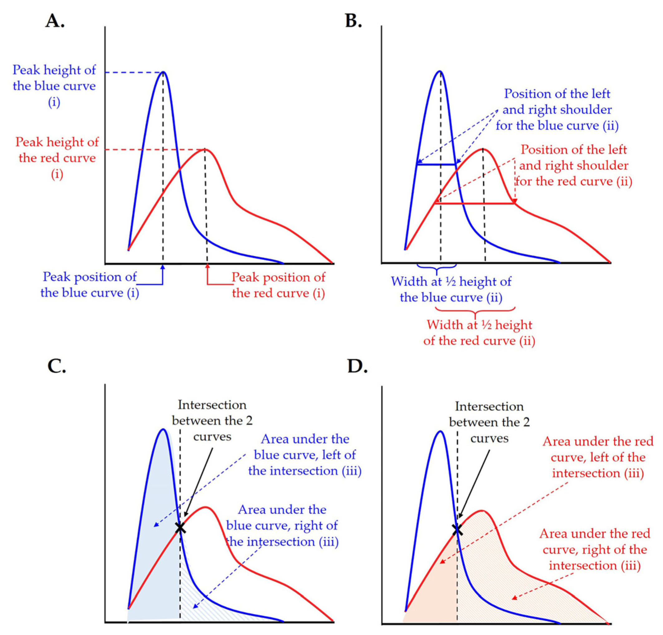
2.3.2. Statistical Analysis of the Results
2.3.3. Plotting and Visualization of the Distribution of Enlarged Airspaces
3. Results
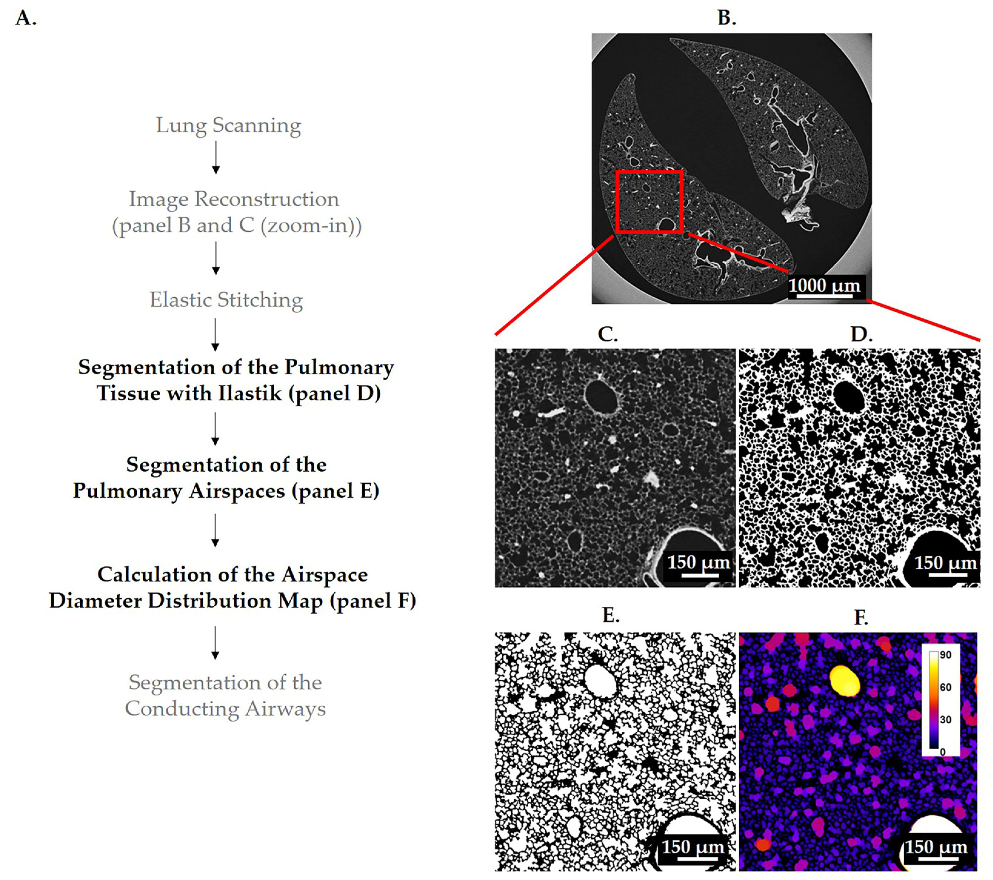
3.1. Segmentations
3.1.1. Segmentation of Pulmonary Tissue
3.1.2. Segmentation of Pulmonary Airspaces
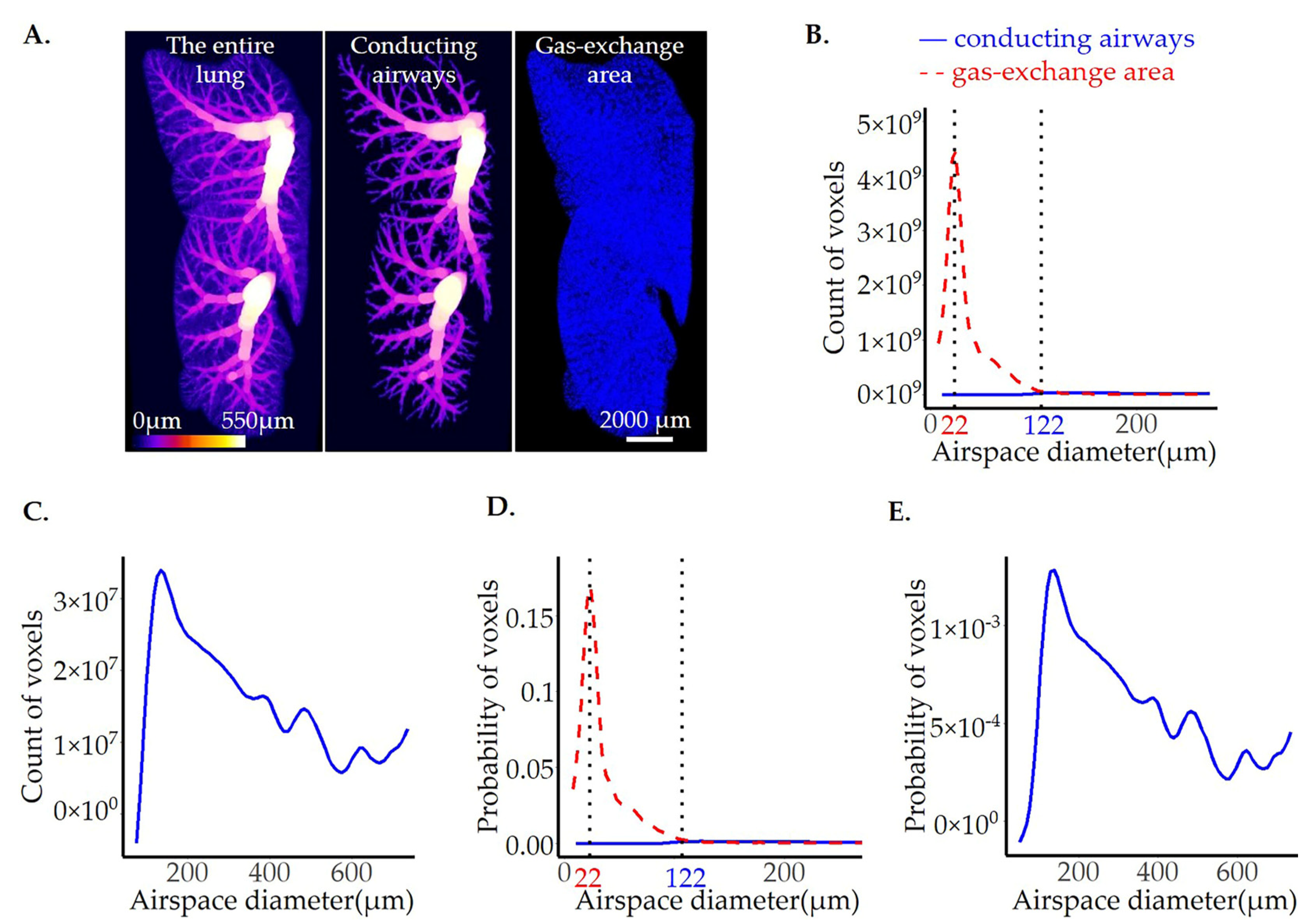
3.2. Calculation of Airspace Diameter Distribution Using the Thickness Map Algorithm
3.3. Extraction of the Conducting Airways
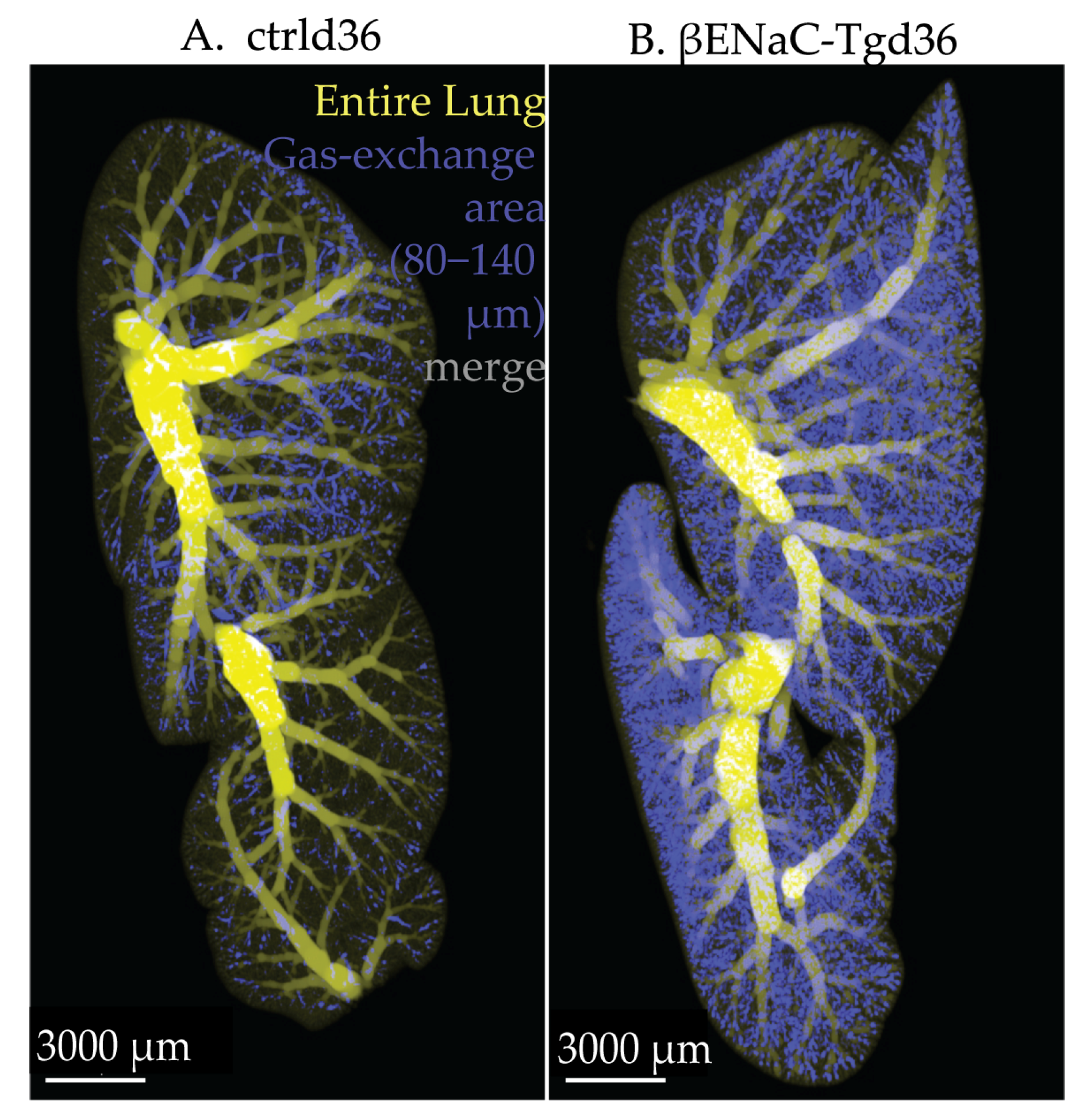
3.4. Airspace Diameter Map of the βENaC-Tg Lungs Scanned by SRXTM
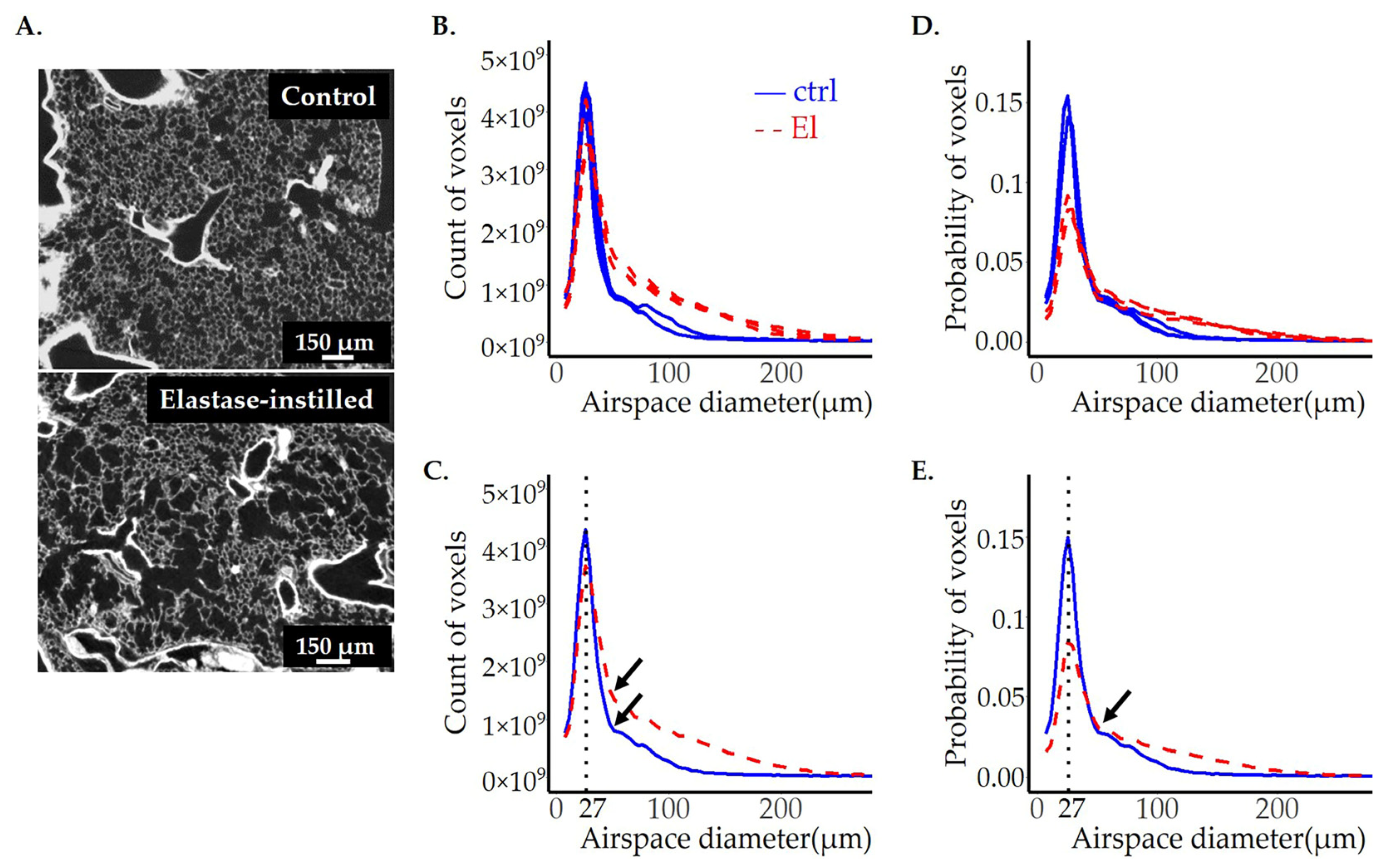
3.5. Airspace Diameter Map of Emphysematous Lungs Scanned by SRXTM
3.6. Comparison of Image Analysis Results of Emphysematous Lungs Scanned by SRXTM and CT—The Impact of Data Quality on Image Analysis Output
4. Discussion
5. Conclusions
Supplementary Materials
Author Contributions
Funding
Institutional Review Board Statement
Informed Consent Statement
Data Availability Statement
Acknowledgments
Conflicts of Interest
References
- Dempsey, T.M.; Scanlon, P.D. Pulmonary Function Tests for the Generalist: A Brief Review. Mayo Clin. Proc. 2018, 93, 763–771. [Google Scholar] [CrossRef]
- Gefter, W.B.; Lee, K.S.; Schiebler, M.L.; Parraga, G.; Seo, J.B.; Ohno, Y.; Hatabu, H. Pulmonary Functional Imaging: Part 2-State-of-the-Art Clinical Applications and Opportunities for Improved Patient Care. Radiology 2021, 299, 524–538. [Google Scholar] [CrossRef]
- Liu, H.; Chen, R.; Tong, C.; Liang, X.W. MRI versus CT for the detection of pulmonary nodules: A meta-analysis. Medicine 2021, 100, e27270. [Google Scholar] [CrossRef]
- Pfeiffer, F.; Bech, M.; Bunk, O.; Kraft, P.; Eikenberry, E.F.; Bronnimann, C.; Grunzweig, C.; David, C. Hard-X-ray dark-field imaging using a grating interferometer. Nat. Mater. 2008, 7, 134–137. [Google Scholar] [CrossRef]
- Hellbach, K.; Yaroshenko, A.; Meinel, F.G.; Yildirim, A.O.; Conlon, T.M.; Bech, M.; Mueller, M.; Velroyen, A.; Notohamiprodjo, M.; Bamberg, F.; et al. In Vivo Dark-Field Radiography for Early Diagnosis and Staging of Pulmonary Emphysema. Investig. Radiol. 2015, 50, 430–435. [Google Scholar] [CrossRef]
- Willer, K.; Fingerle, A.A.; Noichl, W.; De Marco, F.; Frank, M.; Urban, T.; Schick, R.; Gustschin, A.; Gleich, B.; Herzen, J.; et al. X-ray dark-field chest imaging for detection and quantification of emphysema in patients with chronic obstructive pulmonary disease: A diagnostic accuracy study. Lancet Digit. Health 2021, 3, e733–e744. [Google Scholar] [CrossRef]
- Hellbach, K.; Yaroshenko, A.; Willer, K.; Conlon, T.M.; Braunagel, M.B.; Auweter, S.; Yildirim, A.O.; Eickelberg, O.; Pfeiffer, F.; Reiser, M.F.; et al. X-ray dark-field radiography facilitates the diagnosis of pulmonary fibrosis in a mouse model. Sci. Rep. 2017, 7, 340. [Google Scholar] [CrossRef]
- Dubsky, S.; Hooper, S.B.; Siu, K.K.; Fouras, A. Synchrotron-based dynamic computed tomography of tissue motion for regional lung function measurement. J. R. Soc. Interface 2012, 9, 2213–2224. [Google Scholar] [CrossRef]
- Fouras, A.; Allison, B.J.; Kitchen, M.J.; Dubsky, S.; Nguyen, J.; Hourigan, K.; Siu, K.K.; Lewis, R.A.; Wallace, M.J.; Hooper, S.B. Altered lung motion is a sensitive indicator of regional lung disease. Ann. Biomed. Eng. 2012, 40, 1160–1169. [Google Scholar] [CrossRef]
- Kirkness, J.P.; Dusting, J.; Eikelis, N.; Pirakalathanan, P.; DeMarco, J.; Shiao, S.L.; Fouras, A. Association of x-ray velocimetry (XV) ventilation analysis compared to spirometry. Front. Med. Technol. 2023, 5, 1148310. [Google Scholar] [CrossRef]
- Rosenow, T.; Oudraad, M.C.; Murray, C.P.; Turkovic, L.; Kuo, W.; de Bruijne, M.; Ranganathan, S.C.; Tiddens, H.A.; Stick, S.M. Australian Respiratory Early Surveillance Team for Cystic Fibrosis. PRAGMA-CF. A Quantitative Structural Lung Disease Computed Tomography Outcome in Young Children with Cystic Fibrosis. Am. J. Respir. Crit. Care Med. 2015, 191, 1158–1165. [Google Scholar] [CrossRef]
- Loeve, M.; van Hal, P.T.; Robinson, P.; de Jong, P.A.; Lequin, M.H.; Hop, W.C.; Williams, T.J.; Nossent, G.D.; Tiddens, H.A. The spectrum of structural abnormalities on CT scans from patients with CF with severe advanced lung disease. Thorax 2009, 64, 876–882. [Google Scholar] [CrossRef]
- Makita, H.; Nasuhara, Y.; Nagai, K.; Ito, Y.; Hasegawa, M.; Betsuyaku, T.; Onodera, Y.; Hizawa, N.; Nishimura, M.; Hokkaido, C.C.S.G. Characterisation of phenotypes based on severity of emphysema in chronic obstructive pulmonary disease. Thorax 2007, 62, 932–937. [Google Scholar] [CrossRef]
- Ford, N.L.; Martin, E.L.; Lewis, J.F.; Veldhuizen, R.A.; Drangova, M.; Holdsworth, D.W. In vivo characterization of lung morphology and function in anesthetized free-breathing mice using micro-computed tomography. J. Appl. Physiol. (1985) 2007, 102, 2046–2055. [Google Scholar] [CrossRef]
- Namati, E.; Chon, D.; Thiesse, J.; Hoffman, E.A.; de Ryk, J.; Ross, A.; McLennan, G. In vivo micro-CT lung imaging via a computer-controlled intermittent iso-pressure breath hold (IIBH) technique. Phys. Med. Biol. 2006, 51, 6061–6075. [Google Scholar] [CrossRef]
- Schittny, J.C. How high resolution 3-dimensional imaging changes our understanding of postnatal lung development. Histochem. Cell Biol. 2018, 150, 677–691. [Google Scholar] [CrossRef]
- Vasilescu, D.M.; Gao, Z.; Saha, P.K.; Yin, L.; Wang, G.; Haefeli-Bleuer, B.; Ochs, M.; Weibel, E.R.; Hoffman, E.A. Assessment of morphometry of pulmonary acini in mouse lungs by nondestructive imaging using multiscale microcomputed tomography. Proc. Natl. Acad. Sci. USA 2012, 109, 17105–17110. [Google Scholar] [CrossRef]
- McDonough, J.E.; Knudsen, L.; Wright, A.C.; Elliott, W.; Ochs, M.; Hogg, J.C. Regional differences in alveolar density in the human lung are related to lung height. J. Appl. Physiol. (1985) 2015, 118, 1429–1434. [Google Scholar] [CrossRef]
- Barre, S.F.; Haberthur, D.; Cremona, T.P.; Stampanoni, M.; Schittny, J.C. The total number of acini remains constant throughout postnatal rat lung development. Am. J. Physiol. Lung Cell Mol. Physiol. 2016, 311, L1082–L1089. [Google Scholar] [CrossRef]
- Parent, R.A. (Ed.) Comparative Biology of the Normal Lung, 2nd ed.; Academic Press: Cambridge, MA, USA, 2015; p. 815. [Google Scholar] [CrossRef]
- Duerr, J.; Leitz, D.H.W.; Szczygiel, M.; Dvornikov, D.; Fraumann, S.G.; Kreutz, C.; Zadora, P.K.; Seyhan Agircan, A.; Konietzke, P.; Engelmann, T.A.; et al. Conditional deletion of Nedd4-2 in lung epithelial cells causes progressive pulmonary fibrosis in adult mice. Nat. Commun. 2020, 11, 2012. [Google Scholar] [CrossRef] [PubMed]
- Noble, P.W.; Barkauskas, C.E.; Jiang, D. Pulmonary fibrosis: Patterns and perpetrators. J. Clin. Investg. 2012, 122, 2756–2762. [Google Scholar] [CrossRef]
- Pennati, F.; Roach, D.J.; Clancy, J.P.; Brody, A.S.; Fleck, R.J.; Aliverti, A.; Woods, J.C. Assessment of pulmonary structure-function relationships in young children and adolescents with cystic fibrosis by multivolume proton-MRI and CT. J. Magn. Reson. Imaging 2018, 48, 531–542. [Google Scholar] [CrossRef]
- Perossi, J.; Koenigkam-Santos, M.; Perossi, L.; Dos Santos, D.O.; Simoni, L.H.S.; de Souza, H.C.D.; Gastaldi, A.C. Correlation among clinical, functional and morphological indexes of the respiratory system in non-cystic fibrosis bronchiectasis patients. PLoS ONE 2022, 17, e0269897. [Google Scholar] [CrossRef]
- Sallon, C.; Soulet, D.; Provost, P.R.; Tremblay, Y. Automated High-Performance Analysis of Lung Morphometry. Am. J. Respir. Cell Mol. Biol. 2015, 53, 149–158. [Google Scholar] [CrossRef]
- Ochoa, L.F.; Kholodnykh, A.; Villarreal, P.; Tian, B.; Pal, R.; Freiberg, A.N.; Brasier, A.R.; Motamedi, M.; Vargas, G. Imaging of Murine Whole Lung Fibrosis by Large Scale 3D Microscopy aided by Tissue Optical Clearing. Sci. Rep. 2018, 8, 13348. [Google Scholar] [CrossRef]
- Borisova, E.; Lovric, G.; Miettinen, A.; Fardin, L.; Bayat, S.; Larsson, A.; Stampanoni, M.; Schittny, J.C.; Schleputz, C.M. Micrometer-resolution X-ray tomographic full-volume reconstruction of an intact post-mortem juvenile rat lung. Histochem. Cell Biol. 2021, 155, 215–226. [Google Scholar] [CrossRef]
- Mall, M.; Grubb, B.R.; Harkema, J.R.; O’Neal, W.K.; Boucher, R.C. Increased airway epithelial Na+ absorption produces cystic fibrosis-like lung disease in mice. Nat. Med. 2004, 10, 487–493. [Google Scholar] [CrossRef]
- Blaskovic, S.; Donati, Y.; Ruchonnet-Metrailler, I.; Avila, Y.; Schittny, D.; Schleputz, C.M.; Schittny, J.C.; Barazzone-Argiroffo, C. Early life exposure to nicotine modifies lung gene response after elastase-induced emphysema. Respir. Res. 2022, 23, 44. [Google Scholar] [CrossRef]
- Savant, A.; Lyman, B.; Bojanowski, C.; Upadia, J. Cystic Fibrosis. In GeneReviews(®); Adam, M.P., Mirzaa, G.M., Pagon, R.A., Wallace, S.E., Bean, L.J.H., Gripp, K.W., Amemiya, A., Eds.; University of Washington: Seattle, WA, USA, 2023. [Google Scholar]
- Suki, B.; Bartolak-Suki, E.; Rocco, P.R.M. Elastase-Induced Lung Emphysema Models in Mice. Methods Mol. Biol. 2017, 1639, 67–75. [Google Scholar] [CrossRef]
- Percie du Sert, N.; Ahluwalia, A.; Alam, S.; Avey, M.T.; Baker, M.; Browne, W.J.; Clark, A.; Cuthill, I.C.; Dirnagl, U.; Emerson, M.; et al. Reporting animal research: Explanation and elaboration for the ARRIVE guidelines 2.0. PLoS Biol. 2020, 18, e3000411. [Google Scholar] [CrossRef]
- Barre, S.F.; Haberthur, D.; Stampanoni, M.; Schittny, J.C. Efficient estimation of the total number of acini in adult rat lung. Physiol. Rep. 2014, 2, e12063. [Google Scholar] [CrossRef] [PubMed]
- Scherle, W. A simple method for volumetry of organs in quantitative stereology. Mikroskopie 1970, 26, 57–60. [Google Scholar]
- Van Nieuwenhove, V.; De Beenhouwer, J.; De Carlo, F.; Mancini, L.; Marone, F.; Sijbers, J. Dynamic intensity normalization using eigen flat fields in X-ray imaging. Opt. Express 2015, 23, 27975–27989. [Google Scholar] [CrossRef]
- Paganin, D.; Mayo, S.C.; Gureyev, T.E.; Miller, P.R.; Wilkins, S.W. Simultaneous phase and amplitude extraction from a single defocused image of a homogeneous object. J. Microsc. 2002, 206, 33–40. [Google Scholar] [CrossRef]
- Dowd, B.A.; Campbell, G.H.; Marr, R.B.; Nagarkar, V.; Tipnis, S.; Axe, L.; Siddons, D.P. Developments in synchrotron x-ray computed microtomography at the National Synchrotron Light Source. Proc. Soc. Photo-Opt. Instrum. 1999, 3772, 224–236. [Google Scholar] [CrossRef]
- Hadley, W. ggplot2: Elegant Graphics for Data Analysis; Springer: New York, NY, USA, 2016. [Google Scholar]
- R Development Core Team. R: A Language and Environment for Statistical Computing; R Foundation for Statistical Computing: Vienna, Austria, 2010. [Google Scholar]
- Wikipedia. Linear Interpolation. Available online: https://en.wikipedia.org/wiki/Linear_interpolation (accessed on 13 June 2022).
- Wood, S.N. Fast stable restricted maximum likelihood and marginal likelihood estimation of semiparametric generalized linear models. J. R. Stat. Soc. Ser. B Stat. Methodol. 2011, 73, 3–36. [Google Scholar] [CrossRef]
- Berg, S.; Kutra, D.; Kroeger, T.; Straehle, C.N.; Kausler, B.X.; Haubold, C.; Schiegg, M.; Ales, J.; Beier, T.; Rudy, M.; et al. ilastik: Interactive machine learning for (bio)image analysis. Nat. Methods 2019, 16, 1226–1232. [Google Scholar] [CrossRef]
- Schindelin, J.; Arganda-Carreras, I.; Frise, E.; Kaynig, V.; Longair, M.; Pietzsch, T.; Preibisch, S.; Rueden, C.; Saalfeld, S.; Schmid, B.; et al. Fiji: An open-source platform for biological-image analysis. Nat. Methods 2012, 9, 676–682. [Google Scholar] [CrossRef]
- Liu, Y.; Jin, D.; Li, C.; Janz, K.F.; Burns, T.L.; Torner, J.C.; Levy, S.M.; Saha, P.K. A robust algorithm for thickness computation at low resolution and its application to in vivo trabecular bone CT imaging. IEEE Trans. Bio-Med. Eng. 2014, 61, 2057–2069. [Google Scholar] [CrossRef]
- Tran, H.; Doumalin, P.; Delisee, C.; Dupre, J.C.; Malvestio, J.; Germaneau, A. 3D mechanical analysis of low-density wood-based fiberboards by X-ray microcomputed tomography and Digital Volume Correlation. J. Mater. Sci. 2012, 48, 3198–3212. [Google Scholar] [CrossRef]
- Lovric, G.; Vogiatzis Oikonomidis, I.; Mokso, R.; Stampanoni, M.; Roth-Kleiner, M.; Schittny, J.C. Automated computer-assisted quantitative analysis of intact murine lungs at the alveolar scale. PLoS ONE 2017, 12, e0183979. [Google Scholar] [CrossRef]
- Tschanz, S.A.; Salm, L.A.; Roth-Kleiner, M.; Barre, S.F.; Burri, P.H.; Schittny, J.C. Rat lungs show a biphasic formation of new alveoli during postnatal development. J. Appl. Physiol. 2014, 117, 89–95. [Google Scholar] [CrossRef]
- Schittny, J.C. Development of the lung. Cell Tissue Res. 2017, 367, 427–444. [Google Scholar] [CrossRef]
- Agusti, A.; Vogelmeier, C.; Faner, R. COPD 2020: Changes and challenges. Am. J. Physiol. Lung Cell. Mol. Physiol. 2020, 319, L879–L883. [Google Scholar] [CrossRef]
- Barnes, P.J. COPD 2020: New directions needed. Am. J. Physiol. Lung Cell. Mol. Physiol. 2020, 319, L884–L886. [Google Scholar] [CrossRef]
- Suzuki, M.; Betsuyaku, T.; Ito, Y.; Nagai, K.; Odajima, N.; Moriyama, C.; Nasuhara, Y.; Nishimura, M. Curcumin attenuates elastase- and cigarette smoke-induced pulmonary emphysema in mice. Am. J. Physiol. Lung Cell Mol. Physiol. 2009, 296, L614–L623. [Google Scholar] [CrossRef]
- Fysikopoulos, A.; Seimetz, M.; Hadzic, S.; Knoepp, F.; Wu, C.Y.; Malkmus, K.; Wilhelm, J.; Pichl, A.; Bednorz, M.; Tadele Roxlau, E.; et al. Amelioration of elastase-induced lung emphysema and reversal of pulmonary hypertension by pharmacological iNOS inhibition in mice. Br. J. Pharmacol. 2021, 178, 152–171. [Google Scholar] [CrossRef]
- Andersen, M.P.; Parham, A.R.; Waldrep, J.C.; McKenzie, W.N.; Dhand, R. Alveolar fractal box dimension inversely correlates with mean linear intercept in mice with elastase-induced emphysema. Int. J. Chron. Obstruct. Pulmon. Dis. 2012, 7, 235–243. [Google Scholar] [CrossRef]
- Carraro, G.; Langerman, J.; Sabri, S.; Lorenzana, Z.; Purkayastha, A.; Zhang, G.; Konda, B.; Aros, C.J.; Calvert, B.A.; Szymaniak, A.; et al. Transcriptional analysis of cystic fibrosis airways at single-cell resolution reveals altered epithelial cell states and composition. Nat. Med. 2021, 27, 806–814. [Google Scholar] [CrossRef]
- Gehrig, S.; Duerr, J.; Weitnauer, M.; Wagner, C.J.; Graeber, S.Y.; Schatterny, J.; Hirtz, S.; Belaaouaj, A.; Dalpke, A.H.; Schultz, C.; et al. Lack of neutrophil elastase reduces inflammation, mucus hypersecretion, and emphysema, but not mucus obstruction, in mice with cystic fibrosis-like lung disease. Am. J. Respir. Crit. Care Med. 2014, 189, 1082–1092. [Google Scholar] [CrossRef]
- Mansell, A.; Dubrawsky, C.; Levison, H.; Bryan, A.C.; Crozier, D.N. Lung elastic recoil in cystic fibrosis. Am. Rev. Respir. Dis. 1974, 109, 190–197. [Google Scholar] [CrossRef]
- Zhu, L.; Duerr, J.; Zhou-Suckow, Z.; Wagner, W.; Weinheimer, O.; Salomon, J.; Leitz, D.; Konietzke, P.; Yu, H.; Ackermann, M.; et al. microCT to quantify muco-obstructive lung disease and effects of neutrophil elastase knockout in mice. Am. J. Physiol. Lung Cell. Mol. Physiol. 2022, 322, L401–L411. [Google Scholar] [CrossRef]
- Weibel, E.R. Morphometry of the Human Lung; Academic Press: New York, NY, USA, 1963. [Google Scholar]
- Michaudel, C.; Fauconnier, L.; Jule, Y.; Ryffel, B. Functional and morphological differences of the lung upon acute and chronic ozone exposure in mice. Sci. Rep. 2018, 8, 10611. [Google Scholar] [CrossRef]
- Hwang, J.; Kim, M.; Kim, S.; Lee, J. Quantifying morphological parameters of the terminal branching units in a mouse lung by phase contrast synchrotron radiation computed tomography. PLoS ONE 2013, 8, e63552. [Google Scholar] [CrossRef]
- Horsfield, K. Morphology of the bronchial tree in the dog. Respir. Physiol. 1976, 26, 173–182. [Google Scholar] [CrossRef]
- Raabe, O.G.; Yeh, H.C.; Schum, G.M.; Phalen, R.M. Tracheobronchial Geometry: Human, Dog, Rat, Hamster; Lovelace Foundation: Albuquerque, NM, USA, 1976. [Google Scholar]


| Area under the Curve # | |||||||
|---|---|---|---|---|---|---|---|
| Peak Position (µm) | Peak Height | Peak Width at ½ Peak Height (µm) | Before the Curve’s Intersection | After the Curve’s Intersection | Volume of Airspaces (μm3) | ||
| Count | CA | 121.6 | 3.6 × 10⁷ | 160.3 | 2.9 × 10⁸ | 1.8 × 10⁹ | 3.08 × 10¹⁰ |
| GEA | 22.0 | 4.5 × 10⁹ | 17.3 | 1.4 × 10¹⁰ | 1.0 × 10¹⁰ | 3.54 × 10¹¹ | |
| Probability | CA | 121.6 | 1.4 × 10⁻³ | 160.3 | 0.02 | 0.06 | |
| GEA | 22.0 | 0.2 | 17.3 | 0.6 | 0.3 | ||
| Area under the Curve # | |||||||
|---|---|---|---|---|---|---|---|
| Peak Position (µm) | Peak Height | Peak Width at ½ Peak Height (µm) | Before the Curve’s Intersection | After the Curve’s Intersection | Volume of Airspaces (μm3) | ||
| Count | ctrl | 22.0 (0.0) | 3.8 × 10⁹ (9.5 × 10⁸) | 17.1 (0.3) | 1.2 × 10¹⁰ (3.0 × 10⁹) | 1.0 × 10¹⁰ (2.3 × 10⁹) | 3.2 × 10¹¹ (7.7 × 10¹⁰) |
| βENaC-Tg | 35.0 (5.6) | 4.1 × 10⁹ (2.8 × 10⁸) | 30.0 (1.9) | 9.2 × 10⁹ (9.4 × 10⁸) | 3.6 × 10¹⁰ (5.8 × 10⁹) | 6.6 × 10¹¹ (7.3 × 10¹⁰) | |
| p | 0.02 * | 0.6 | 0.0003 *** | 0.2 | 0.002 ** | 0.005 ** | |
| Probability | ctrl | 22.0 (0.0) | 0.17 (0.003) | 17.1 (0.3) | 0.5 (0.01) | 0.5 (0.01) | |
| βENaC-Tg | 35.0 (5.6) | 0.09 (0.007) | 30.0 (1.9) | 0.2 (0.04) | 0.8 (0.04) | ||
| p | 0.02 * | 4.6 × 10⁻⁵ **** | 0.0003 *** | 0.0002n *** | 0.0002 *** | ||
| Area under the Curve # | |||||||
|---|---|---|---|---|---|---|---|
| Peak Position (µm) | Peak Height | Peak Width at ½ Peak Height (µm) | Before the Curve’s Shoulder | Curve’s Shoulder Till End | Volume of Airspaces (μm3) | ||
| Count | ctrl | 26.9 (0.0) | 4.2 × 10⁹ (3.4 × 10⁸) | 13.1 (0.2) | 1.9 × 10¹⁰ (1.5 × 10⁹) | 1.0 × 10¹⁰ (1.5 × 10⁹) | 4.2 × 10¹¹ (4.0 × 10¹⁰) |
| El | 26.9 (0.0) | 3.7 × 10⁹ (4.1 × 10⁸) | 18.0 (1.4) | 1.8 × 10¹⁰ (1.7 × 10⁹) | 2.5 × 10¹⁰ (1.3 × 10⁹) | 6.3 × 10¹¹ (4.1 × 10¹⁰) | |
| p | 0.4 | 0.2 | 0.004 ** | 0.7 | 0.0002 *** | 0.002 ** | |
| Probability | ctrl | 26.9 (0.0) | 0.15 (0.003) | 13.1 (0.2) | 0.6 (0.02) | 0.4 (0.02) | |
| El | 26.9 (0.0) | 0.09 (0.005) | 18.0 (1.4) | 0.4 (0.02) | 0.6 (0.02) | ||
| p | 0.4 | 6.6 × 10⁻⁵ **** | 0.004 ** | 0.0001 *** | 0.0001 *** | ||
| Area under the Curve | |||||||
|---|---|---|---|---|---|---|---|
| Peak Position (µm) | Peak Height | Peak Width at ½ Peak Height (µm) | Before the Shoulder | Shoulder | After Shoulder | ||
| ctrl | SRXTM | 22.0 | 0.17 | 17.7 | 0.7 | 0.2 | 0.1 |
| μCT | 24.8 | 0.16 | 19.1 | 0.7 | 0.2 | 0.1 | |
| El-1 | SRXTM | 26.9 | 0.09 | 26.4 | 0.43 | 0.5 | 0.03 |
| μCT | 20.3 | 0.08 | 27.8 | 0.46 | 0.5 | 0.03 | |
| El-2 | SRXTM | 22.0 | 0.15 | 19.7 | 0.7 | 0.2 | 0.1 |
| μCT | 20.3 | 0.16 | 19.8 | 0.8 | 0.1 | 0.1 | |
Disclaimer/Publisher’s Note: The statements, opinions and data contained in all publications are solely those of the individual author(s) and contributor(s) and not of MDPI and/or the editor(s). MDPI and/or the editor(s) disclaim responsibility for any injury to people or property resulting from any ideas, methods, instructions or products referred to in the content. |
© 2023 by the authors. Licensee MDPI, Basel, Switzerland. This article is an open access article distributed under the terms and conditions of the Creative Commons Attribution (CC BY) license (https://creativecommons.org/licenses/by/4.0/).
Share and Cite
Blaskovic, S.; Anagnostopoulou, P.; Borisova, E.; Schittny, D.; Donati, Y.; Haberthür, D.; Zhou-Suckow, Z.; Mall, M.A.; Schlepütz, C.M.; Stampanoni, M.; et al. Airspace Diameter Map—A Quantitative Measurement of All Pulmonary Airspaces to Characterize Structural Lung Diseases. Cells 2023, 12, 2375. https://doi.org/10.3390/cells12192375
Blaskovic S, Anagnostopoulou P, Borisova E, Schittny D, Donati Y, Haberthür D, Zhou-Suckow Z, Mall MA, Schlepütz CM, Stampanoni M, et al. Airspace Diameter Map—A Quantitative Measurement of All Pulmonary Airspaces to Characterize Structural Lung Diseases. Cells. 2023; 12(19):2375. https://doi.org/10.3390/cells12192375
Chicago/Turabian StyleBlaskovic, Sanja, Pinelopi Anagnostopoulou, Elena Borisova, Dominik Schittny, Yves Donati, David Haberthür, Zhe Zhou-Suckow, Marcus A. Mall, Christian M. Schlepütz, Marco Stampanoni, and et al. 2023. "Airspace Diameter Map—A Quantitative Measurement of All Pulmonary Airspaces to Characterize Structural Lung Diseases" Cells 12, no. 19: 2375. https://doi.org/10.3390/cells12192375
APA StyleBlaskovic, S., Anagnostopoulou, P., Borisova, E., Schittny, D., Donati, Y., Haberthür, D., Zhou-Suckow, Z., Mall, M. A., Schlepütz, C. M., Stampanoni, M., Barazzone-Argiroffo, C., & Schittny, J. C. (2023). Airspace Diameter Map—A Quantitative Measurement of All Pulmonary Airspaces to Characterize Structural Lung Diseases. Cells, 12(19), 2375. https://doi.org/10.3390/cells12192375