Estimation of Cotton Aboveground Biomass Based on UAV Multispectral Images: Multi-Feature Fusion and CNN Model

Abstract

Precise estimation of cotton aboveground biomass (AGB) plays a crucial role in effectively analyzing growth variations and development of cotton, as well as guiding agricultural management practices. Multispectral (MS) sensors mounted on UAVs offer a practical and accurate approach for estimating the AGB of cotton. Many previous studies have mainly emphasized the combination of spectral and texture features, as well as canopy height (CH). However, current research overlooks the potential of integrating spectral, textural features, and CH to estimate AGB. In addition, the accumulation of AGB often exhibits synergistic effects rather than a simple additive relationship. Conventional algorithms, including Bayesian Ridge Regression (BRR) and Random Forest Regression (RFR), often fail to accurately capture the nonlinear and intricate correlations between biomass and its relevant variables. Therefore, this research develops a method to estimate cotton AGB by integrating multiple feature information with a deep learning model. Spectral and texture features were derived from MS images. Cotton CH extracted from UAV point cloud data. Variables of multiple features were selected using Spearman’s Correlation (SC) coefficients and the variance inflation factor (VIF). Convolutional neural network (CNN) was chosen to build a model for estimating cotton AGB and contrasted with traditional machine learning models (RFR and BRR). The results indicated that (1) combining spectral, textural features, and CH yielded the highest precision in cotton AGB estimation; (2) compared to traditional ML models (RFR and BRR), the accuracy of applying CNN for estimating cotton AGB is better. CNN has more advanced power to learn complex nonlinear relationships among cotton AGB and multiple features; (3) the most effective strategy in this study involves combining spectral, texture features, and CH, selecting variables using the SC and VIF methods, and employing CNN for estimating AGB of cotton. The R² of this model is 0.80, with an RMSE of 0.17 kg·m⁻² and an MAE of 0.11 kg·m⁻². This study develops a framework for evaluating cotton AGB by multiple features fusion with a deep learning model. It provides technical support for monitoring crop growth and improving field management.

1. Introduction

Cotton is a valuable cash crop [1], being extensively employed for textiles, garments, and various industrial goods all over the world. It has great economic and social significance [2]. Aboveground biomass (AGB) serves as an important parameter for assessing the growth condition of cotton and has a direct influence on its yield and quality [3,4]. Thus, to monitor growth and development of cotton, predict its yield [5], and guide production practices [6], a precise estimation of AGB is necessary. Traditional methods of cotton AGB measurement rely on field sampling and weighing, which are time and labor-consuming. They are not appropriate for large-scale and rapid estimation [7]. Advances in unmanned aerial vehicle (UAV) remote sensing technology have made it technically possible to estimate AGB rapidly and efficiently [8,9]. Multispectral (MS) imagery of the crop canopy by UAV was obtained. The spectral features of MS imagery effectively capture information related to crop growth [10]. The accurate estimation of AGB can be achieved by analyzing the statistical relationship between spectral features and AGB [11]. However, spectral reflectance is more likely to saturate under complex dense vegetation conditions [12], which affects the accuracy of estimating AGB from spectral information. Current research increasingly favors fusing spectral features from UAV images with other features such as texture features and canopy height (CH) to improve AGB estimation accuracy [13,14,15]. Textural features show clear advantages in crop monitoring [16]. Textural features can reveal intricate details of canopy surface structure. The texture image reflects leaf orientation, overlap, and the degree of crowding in the foliage. Typical examples include Gray Level Cooccurrence Matrix (GLCM) metrics such as contrast, homogeneity, and entropy, which reflect canopy roughness, leaf arrangement, and surface heterogeneity [17]. Subtracting the digital elevation model (DEM) from the digital surface model (DSM) yields precise crop canopy height measurements, reflecting the vertical structure of the canopy [18]. CH is a fundamental indicator for characterizing the three-dimensional structure of crops and estimating biomass [19]. Taller crops possess greater dry matter content (biomass) in their stems, branches, and leaves.

In recent years, notable advances have been made in enhancing AGB estimation accuracy by combining multi-features derived from UAV imagery [20,21]. These approaches are generally classified into two main groups. The first type of approach is to fuse spectral and texture features. Spectral features reflect canopy chlorophyll content and leaf size. Textural features reflect canopy surface structure, such as leaf orientation, overlap, and interlacing density [22]. This approach simultaneously accounts for both crop biomass accumulation capacity and the surface structure of the crop canopy. The integration of these spectral and texture features contributes to improving the precision of AGB estimation. Grüner et al. [23] improved the precision of AGB estimation in leguminous crops by combining spectral and textural features derived from multispectral images. Similarly, Xu et al. [24] demonstrated that integrating spectral and textural features extracted from MS imagery improved the accuracy of rice AGB estimation compared with using spectral or textural features alone. This method incorporates additional texture information to overcome the limitations of relying solely on spectral features, which improves the reliability of AGB estimation. However, this approach is limited in its capacity to capture information about the vertical structure of crops, which can lead to either underestimation or overestimation of aboveground biomass (AGB) [25]. Studies have shown that the DSM generated from point clouds can be used to create a crop height model. From these models, CH is extracted as a feature representing the vertical growth of crops. [26]. To address this limitation, researchers have developed a second category of methods that integrate spectral features and CH. This method comprehensively considers spectral features reflecting canopy chlorophyll content and leaf size, as well as canopy height features reflecting vertical canopy structure. It simultaneously accounts for both crop biomass accumulation capacity and crop vertical structure. Yin et al. [27] estimated corn AGB by fusing spectral features and CH from multispectral images, achieving an R² of 0.74. Furthermore, Astor et al. [28] used point clouds of UAV RGB to extract crop height and hyperspectral images to extract spectral reflectance to estimate vegetable biomass and achieved good estimation performance. It addresses the limitations of spectral features in capturing information about vegetation vertical growth. This improvement significantly enhances the accuracy of AGB estimation. This method describes crop growth from two dimensions, but does not fully consider the role of texture features in characterizing canopy surface details. Therefore, methods that integrate spectral, texture, features, and CH from UAV imagery remain a key research focus in the field of AGB estimation. The accuracy of crop AGB estimation based on UAV imagery is influenced not only by multi-feature fusion but also by the choice of algorithm [29,30,31]. Currently, the three commonly used algorithms in this field are Bayesian Ridge Regression (BRR), Random Forest Regression (RFR), and Convolutional Neural Network (CNN) [32,33,34]. Agbona et al. [35] achieved good performance in estimating the AGB of cassava roots using the BRR algorithm. Johansen et al. [36] used the RFR algorithm to build an AGB estimation model. It effectively estimated tomato AGB and yield. Vawda et al. [37] used CNN and artificial neural network (ANN) algorithms to estimate AGB of dry grassland. Results revealed that CNN outperformed ANN with a slightly higher level of accuracy. It is evident that these models have a significant advantage in estimating other crops’ AGB. However, the potential of algorithms for cotton AGB assessment is still unclear.

Overall, two main methods have emerged for evaluating crop AGB based on MS imagery. Methods that integrate spectral and textural features demonstrated stable performance in certain scenarios but were limited in capturing crop height information. Conversely, methods that combine spectral features and CH account for crop height information but ignore textural features. Actually, crop AGB is closely correlated with leaf area, chlorophyll content, leaf size, and plant height. Spectral features are a comprehensive reflection of chlorophyll content and leaf area size [38,39]. Larger leaves and higher chlorophyll content typically indicate stronger photosynthetic capacity, which is conducive to biomass accumulation. Textural features indirectly reflect canopy surface structure through texture metrics such as image roughness and contrast [40]. A more complex and rougher canopy surface structure indicates denser foliage and greater interlacing of branches and leaves. This directly contributes to increased biomass. CH reflects the vertical growth status of crops [41]. Taller plants possess greater dry matter biomass (biomass) in their stems, branches, leaves, and other organs. Evidently, current research has insufficiently considered the integration of multiple features. In addition to considering the integration of the aforementioned multiple features, AGB estimation models must also address the complex nonlinear relationships between multiple features and AGB. Therefore, developing a deep learning framework that captures multiple features, including spectral, textural features, and CH, to increase the accuracy of cotton aboveground biomass models is a critical issue.

The present study focuses on the cotton AGB at Huaxing Farm, located in Changji City, Xinjiang Uygur Autonomous Region, China. Spectral, textural features, and CH were extracted based on multispectral imagery acquired by unmanned aerial vehicles (UAVs). Four image feature combination schemes were established, including (1) spectral features only, (2) spectral combined with textural features, (3) spectral combined with CH, and (4) integrated spectral, textural features, and CH. Furthermore, CNN and traditional machine learning algorithms (RFR and BRR) were each integrated with selected features to develop a cotton AGB prediction model that can be applied throughout the entire growth stage. The research objectives are as follows: (1) to compare the influence of four feature combination schemes on the effect of cotton AGB estimation; (2) to assess the performance of CNN and conventional machine learning algorithms (RFR and BRR) for estimating cotton AGB; and (3) to explore an optimal framework for estimating cotton AGB that combines image feature fusion with modeling algorithms. This research establishes an innovative framework for estimating cotton AGB through the integration of multi-feature fusion and deep learning techniques, providing methodological support for cotton growth monitoring and a reliable technical tool for agricultural management.

2. Materials and Methods

2.1. Research Area and Experimental Design

As presented in Figure 1, the research area lies in Changji City, Changji Hui Autonomous Prefecture, Xinjiang Uygur Autonomous Region, China (87°30′ E, 44°21′ N). This area has an average elevation of about 450 m and belongs to the temperate continental arid climate. Climatic indicators for this region were derived from long-term daily meteorological records obtained from the China Meteorological Administration (China Meteorological Data Service Center) [42]. The accumulated annual temperature above 10 °C is over 3200 °C·d, while the total sunshine hours per year range between 2800 and 3000, and the frost-free duration lasts approximately 170–200 days. This region is characterized by scarce rainfall, with annual precipitation between 150 and 200 mm, while evapotranspiration averages nearly 1500 mm per year. The experimental field soil is clay loam, with organic matter levels of 10–15 g·kg⁻¹, total nitrogen ranging from 0.8 to 1.2 g·kg⁻¹, bulk density between 1.3 and 1.4 g·cm⁻³, and a pH value of 7.5–8.0.

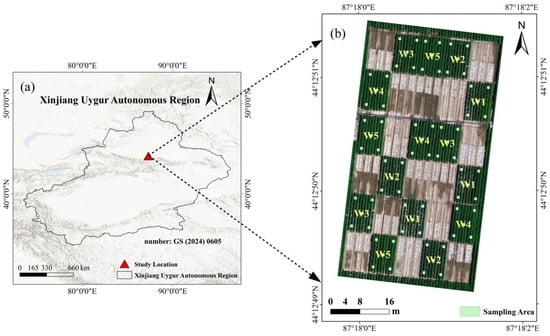
Figure 1. An outline of the research area. (a) Experimental zone; (b) experimental field and experimental design.

2.2. Experimental Design

The field trial was conducted during the 2023 cotton growing season. Despite being limited to one year, the experimental design covered a wide scope of canopy growth and water conditions, providing sufficient variability for model calibration. The cotton variety used in this experiment was Zhongmian 113, an early-maturing conventional upland variety with a growth duration of about 115 days. It was sown around 20 April 2023. A randomized block design was employed in this study, setting up 5 irrigation treatments, with each treatment replicated 3 times, for a total of 15 plots (Figure 1). Each plot is separated by a 1 m or 0.5 m protective barrier. This arrangement guaranteed statistical reliability and successfully reduced random errors. The experiment was designed with five irrigation levels based on the field irrigation amount. Using local field irrigation volume as the reference baseline, (100%) represented the local field irrigation volume amount, and the other treatments (W1–W3 and W5) were set as fixed proportions of this standard amount (17%, 33%, 67%, and 133%). The experimental fields’ planting densities and fertilization techniques, with the exception of irrigation levels, were in line with standard field management techniques. The study area has low rainfall and high evaporation. Rainfall in the experimental field can be considered evenly distributed. Therefore, the influence of rainfall on this experiment can be ignored.

2.3. Cotton AGB Data Collection

To capture the dynamic patterns of cotton growth, cotton AGB data collection covered five key growth stages: seedling stage, squaring stage, flowering stage, boll setting stage, and boll opening stage. Five 1 m² sample plots were chosen from each plot after each drone image was taken. Three cotton plants that were all growing at the same rate were chosen from each plot at random. The number of cotton plants in the sample area was counted. This method of sampling was much more representative and accurate, which reduced the chance of random errors that can happen with a single sampling point. Selected cotton plants were cut at the base near the ground. They were then chopped into small pieces and placed in paper bags. The samples were first dried at 105 °C for 30 min, subsequently cooled to 80 °C, and further dried until a constant weight was achieved. Weigh the dried cotton sample and record the dry weight. AGB was derived from the count of cotton plants in each sample plot and their mean individual weight. After five data collections based on ground, this study obtained 375 measured data points for cotton AGB. The statistical characteristics of the measured cotton AGB data for the total sample set are shown in Table 1. Although this study collected data for only one year, the experimental design covered a wide scope of biomass variation from low to high. It effectively captured the dynamic changes in AGB throughout the entire growth period of cotton.

Table 1. Statistical characteristics of the total sample set for cotton aboveground biomass (AGB) data.

Dataset	Sample Size	Mean (kg·m−2)	Maximum (kg·m−2)	Minimum (kg·m−2)	Standard Deviation (kg·m−2)	Variance	Coefficient of Variation
Total sample set	375	0.51	1.80	0.05	0.39	0.15	0.77

2.4. UAV Data Acquisition and Preprocessing

UAV data collection also covers five key growth stages of cotton. A DJI M300 RTK unmanned aerial vehicle (Matrice 300 Real-Time Kinematic, DJI Innovation Technology Co., Ltd., Shenzhen, China) was utilized in this experiment. The UAV system was fitted with an MS600 Pro multispectral camera (YUSENSE (Changguang Yuchen) Co., Ltd., Qingdao, China) that provides an image resolution of 1.2 megapixels. The MS600 Pro multispectral sensor features six bands: blue, green, red, near-infrared, red edge 1, and red edge 2. The center wavelengths for each band are 450 nm, 555 nm, 660 nm, 840 nm, 720 nm, and 750 nm, respectively. UAV imagery was collected from 13:00 to 15:00 under stable atmospheric conditions with clear skies and no wind. Radiometric calibration was conducted prior to each flight. Each drone flight occurs prior to cotton AGB data collection. The drone flight level is 15 m, with a ground resolution of 0.01 m. Both the front and side overlaps are 80%. As shown in Figure 2, there are three rows of cotton in a plastic film. At this ground resolution, cotton rows can be clearly distinguished. The resolution is sufficient and reliable for extracting cotton plant height data. Detailed imaging times and parameter settings are provided in Table 2.

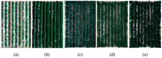
Figure 2. UAV RGB (true color) images of a representative cotton plot acquired at the cotton growth stage. (a) Seedling stage, (b) squaring stage, (c) flowering stage, (d) boll setting stage, and (e) boll opening stage.

Table 2. Drone flight duration and parameter settings.

Image Data Acquisition Time	Growing Stage of Cotton	Time Since Emergence (Day)	Drone Platform Model	Sensor Model	Flight Level (m)	Ground Resolution (m)	Front and Side Overlap
20 April 2023	bare soil stage	-	M300RTK	MS600PRO	15	0.01	80% + 80%
14 June 2023	seedling stage	44			15	0.01	80% + 80%
28 June 2023	squaring stage	58			15	0.01	80% + 80%
18 July 2023	flowering stage	78			15	0.01	80% + 80%
2 August 2023	boll setting stage	92			15	0.01	80% + 80%
22 August 2023	boll opening stage	112			15	0.01	80% + 80%

Upon completion of the UAV flight, radiometric correction was carried out with Yusense Ref software (version 3.2, YUSENSE (Changguang Yuchen) Co., Ltd., Qingdao, China). Subsequently, Pix4D Mapper software (version 4.5.6, Pix4D S.A., Prilly, Switzerland) was used for multispectral image stitching. For each flight image, six single-band reflectance maps and one DSM were generated. Finally, reflectance calibration was conducted in ENVI software (version 5.6, L3Harris Geospatial, Boulder, CO, USA). ArcGIS software (version 10.7, Esri Inc., Redlands, CA, USA) was used to generate the Shapefile of the sample plots.

After computing the NDVI of the MS images in Python (version 3.8.20, Python Software Foundation, Wilmington, DE, USA), the Otsu thresholding algorithm was applied to remove the soil background [43]. Subsequent extraction of spectral features, texture features, and CH all removed the soil background.

2.5. Image Feature Extraction

2.5.1. Spectral Feature Extraction

Spectral features were extracted from MS images for five cotton growth stages. The study selected six original bands and 36 vegetation indices (VIs), which are widely used in crop AGB estimation research [44,45,46,47,48,49,50,51,52,53,54,55,56,57,58,59,60]. The definitions and corresponding references for all selected bands and VIs are displayed in Table 3.

Table 3. Spectral index formula for calculation.

Number	Spectral Indices	Definition	Reference
1	B	Blue	-
2	G	Green	-
3	R	Red	-
4	NIR	Nir	-
5	RE1	RedEdge1	-
6	RE2	RedEdge2	-
7	Normalized difference vegetation index (NDVI)	$\mathrm{N}\mathrm{D}\mathrm{V}\mathrm{I}=(\mathrm{N}\mathrm{I}\mathrm{R}-\mathrm{R})/(\mathrm{N}\mathrm{I}\mathrm{R}+\mathrm{R})$	[44]
8	Green-normalized difference vegetation index (GNDVI)	$\mathrm{G}\mathrm{N}\mathrm{D}\mathrm{V}\mathrm{I}=(\mathrm{N}\mathrm{I}\mathrm{R}-\mathrm{G})/(\mathrm{N}\mathrm{I}\mathrm{R}+\mathrm{G})$	[45]
9	Triangular vegetation index (TVI)	$\mathrm{T}\mathrm{V}\mathrm{I}=60\times (\mathrm{N}\mathrm{I}\mathrm{R}-\mathrm{G})-100\times (\mathrm{R}-\mathrm{G})$	[46]
10	Optimized soil-adjusted vegetation index (OSAVI)	$\mathrm{O}\mathrm{S}\mathrm{A}\mathrm{V}\mathrm{I}=1.16\times (\mathrm{N}\mathrm{I}\mathrm{R}-\mathrm{R})/(\mathrm{N}\mathrm{I}\mathrm{R}+\mathrm{R}+0.16)$	[47]
11	Soil-adjusted vegetation index (SAVI)	$\mathrm{S}\mathrm{A}\mathrm{V}\mathrm{I}=1.5\times (\mathrm{N}\mathrm{I}\mathrm{R}-\mathrm{R})/(\mathrm{N}\mathrm{I}\mathrm{R}+\mathrm{R}+0.5)$	[48]
12	Ratio vegetation index (RVI)	$\mathrm{R}\mathrm{V}\mathrm{I}=\mathrm{N}\mathrm{I}\mathrm{R}/\mathrm{R}$	[49]
13	Ratio vegetation index 2 (RVI2)	$\mathrm{R}\mathrm{V}\mathrm{I}2=\mathrm{N}\mathrm{I}\mathrm{R}/\mathrm{G}$	[50]
14	Enhanced vegetation index (EVI)	$\mathrm{E}\mathrm{V}\mathrm{I}=2.5\times (\mathrm{N}\mathrm{I}\mathrm{R}-\mathrm{R})/(\mathrm{N}\mathrm{I}\mathrm{R}+6\times \mathrm{R}-7.5\times \mathrm{B}+1)$	[51]
15	Green chlorophyll index (GCI)	$\mathrm{G}\mathrm{C}\mathrm{I}=(\mathrm{N}\mathrm{I}\mathrm{R}/\mathrm{G})-1$	[52]
16	Red-edge1 chlorophyll index (RECI1)	$\mathrm{R}\mathrm{E}\mathrm{C}\mathrm{I}1=(\mathrm{N}\mathrm{I}\mathrm{R}/\mathrm{R}\mathrm{E}1)-1$	[52]
17	Red-edge2 chlorophyll index 2 (RECI2)	$\mathrm{R}\mathrm{E}\mathrm{C}\mathrm{I}2=(\mathrm{N}\mathrm{I}\mathrm{R}/\mathrm{R}\mathrm{E}2)-1$	[52]
18	Green–red vegetation index (GRVI)	$\mathrm{G}\mathrm{R}\mathrm{V}\mathrm{I}=(\mathrm{G}-\mathrm{R})/(\mathrm{G}+\mathrm{R})$	[53]
19	Normalized difference vegetation index 2 (NDVIgb)	$\mathrm{N}\mathrm{D}\mathrm{V}\mathrm{I}\mathrm{g}\mathrm{b}=(\mathrm{G}-\mathrm{B})/(\mathrm{G}+\mathrm{B})$	[54]
20	Normalized difference red-edge1 (NDRE1)	$\mathrm{N}\mathrm{D}\mathrm{R}\mathrm{E}1=(\mathrm{N}\mathrm{I}\mathrm{R}-\mathrm{R}\mathrm{E}1)/(\mathrm{N}\mathrm{I}\mathrm{R}+\mathrm{R}\mathrm{E}1)$	[55]
21	Normalized difference red-edge2 (NDRE2)	$\mathrm{N}\mathrm{D}\mathrm{R}\mathrm{E}2=(\mathrm{N}\mathrm{I}\mathrm{R}-\mathrm{R}\mathrm{E}2)/(\mathrm{N}\mathrm{I}\mathrm{R}+\mathrm{R}\mathrm{E}2)$	[55]
22	Normalized difference red-edge1 index (NDREI1)	$\mathrm{N}\mathrm{D}\mathrm{R}\mathrm{E}\mathrm{I}1=(\mathrm{R}\mathrm{E}1-\mathrm{G})/(\mathrm{R}\mathrm{E}1+\mathrm{G})$	[56]
23	Normalized difference red-edge2 index 2 (NDREI2)	$\mathrm{N}\mathrm{D}\mathrm{R}\mathrm{E}\mathrm{I}2=(\mathrm{R}\mathrm{E}2-\mathrm{G})/(\mathrm{R}\mathrm{E}2+\mathrm{G})$	[57]
24	Simplified canopy chlorophyll content index (SCCCI1)	$\mathrm{S}\mathrm{C}\mathrm{C}\mathrm{C}\mathrm{I}1=\mathrm{N}\mathrm{D}\mathrm{R}\mathrm{E}1/\mathrm{N}\mathrm{D}\mathrm{V}\mathrm{I}$	[57]
25	Simplified canopy chlorophyll content index 2 (SCCCI2)	$\mathrm{S}\mathrm{C}\mathrm{C}\mathrm{C}\mathrm{I}2=\mathrm{N}\mathrm{D}\mathrm{R}\mathrm{E}2/\mathrm{N}\mathrm{D}\mathrm{V}\mathrm{I}$	[57]
26	Optimized soil-adjusted vegetation index 2 (OSAVI1)	$\mathrm{O}\mathrm{S}\mathrm{A}\mathrm{V}\mathrm{I}1=(\mathrm{N}\mathrm{I}\mathrm{R}-\mathrm{R})/(\mathrm{N}\mathrm{I}\mathrm{R}-\mathrm{R}+0.16)$	[47]
27	Modified chlorophyll absorption in reflectance index (MCARI1)	$\mathrm{M}\mathrm{C}\mathrm{A}\mathrm{R}\mathrm{I}1=\left[\right(\mathrm{R}\mathrm{E}1-\mathrm{R})-0.2\times (\mathrm{R}\mathrm{E}1-\mathrm{G}\left)\right]\times (\mathrm{R}\mathrm{E}1/\mathrm{R})$	[58]
28	Modified chlorophyll absorption in reflectance index 2 (MCARI2)	$\mathrm{M}\mathrm{C}\mathrm{A}\mathrm{R}\mathrm{I}2=\left[\right(\mathrm{R}\mathrm{E}2-\mathrm{R})-0.2\times (\mathrm{R}\mathrm{E}2-\mathrm{G}\left)\right]\times (\mathrm{R}\mathrm{E}2/\mathrm{R})$	[58]
29	Transformed chlorophyll absorption in reflectance index (TCARI1)	$\mathrm{T}\mathrm{C}\mathrm{A}\mathrm{R}\mathrm{I}1=3\times \left[\right(\mathrm{R}\mathrm{E}1-\mathrm{R})-0.2\times (\mathrm{R}\mathrm{E}1-\mathrm{G})\times (\mathrm{R}\mathrm{E}1/\mathrm{R}\left)\right]$	[58]
30	Transformed chlorophyll absorption in reflectance index 2 (TCARI2)	$\mathrm{T}\mathrm{C}\mathrm{A}\mathrm{R}\mathrm{I}2=3\times \left[\right(\mathrm{R}\mathrm{E}2-\mathrm{R})-0.2\times (\mathrm{R}\mathrm{E}2-\mathrm{G})\times (\mathrm{R}\mathrm{E}2/\mathrm{R}\left)\right]$	[58]
31	MCARI1/OSAVI2 (M/O2 1)	$\mathrm{M}\mathrm{C}\mathrm{A}\mathrm{R}\mathrm{I}1/\mathrm{O}\mathrm{S}\mathrm{A}\mathrm{V}\mathrm{I}2$	[59]
32	MCARI2/OSAVI2 (M/O2 2)	$\mathrm{M}\mathrm{C}\mathrm{A}\mathrm{R}\mathrm{I}2/\mathrm{O}\mathrm{S}\mathrm{A}\mathrm{V}\mathrm{I}2$	[59]
33	TCARI1/OSAVI2 (T/O2 1)	$\mathrm{T}\mathrm{C}\mathrm{A}\mathrm{R}\mathrm{I}1/\mathrm{O}\mathrm{S}\mathrm{A}\mathrm{V}\mathrm{I}2$	-
34	TCARI2/OSAVI2 (T/O2 2)	$\mathrm{T}\mathrm{C}\mathrm{A}\mathrm{R}\mathrm{I}2/\mathrm{O}\mathrm{S}\mathrm{A}\mathrm{V}\mathrm{I}2$	-
35	Wide dynamic range vegetation index (WDRVI)	$\mathrm{W}\mathrm{D}\mathrm{R}\mathrm{V}\mathrm{I}=(0.12\times \mathrm{N}\mathrm{I}\mathrm{R}-\mathrm{R})/(0.12\times \mathrm{N}\mathrm{I}\mathrm{R}+\mathrm{R})$	[58]
36	Green–red ratio index (GRRI)	$\mathrm{G}\mathrm{R}\mathrm{R}\mathrm{I}=\mathrm{G}/\mathrm{R}$	[60]

2.5.2. Texture Feature Extraction

Textural features were extracted from six spectral bands of multispectral imagery covering five cotton growth stages. Texture features correlate with the repeatability of local patterns in images, reflecting the canopy surface structure. Texture features were extracted from six MS bands using GLCM in ENVI software. A 3 × 3 moving window with a stride of 1 pixel was applied, and texture values were averaged across four directional angles (0°, 45°, 90°, and 135°). For each spectral band, eight texture parameters, including mean (MEA), variance (VAR), homogeneity (HOM), contrast (CON), dissimilarity (DIS), entropy (ENT), angular second moment (ASM), and correlation (COR) [61] were calculated. In total, 48 texture indices were calculated for each sample across the six multispectral bands.

2.5.3. Canopy Height (CH) Extraction

CH reflects the vertical structure of crops. The Structure from Motion (SfM) algorithm for 3D reconstruction utilizes high-density point cloud data to establish DSMs for five stages of cotton growth and the bare soil stage. The DSM of the bare soil period was treated as the DEM. The cotton canopy height model (CHM) is derived from DSM by subtracting DEM [62]. The CHM represents the canopy height of cotton:

$$\mathrm{CHM} = \mathrm{DSM}-\mathrm{D}\mathrm{E}\mathrm{M}$$

(1)

2.6. Method

2.6.1. Image Feature Fusion Method

This study employed three image feature fusion methods. The four image feature fusion methods are feature level fusion, that is simple splicing fusion [63]. In this study, feature variables selected from different feature fusion methods across five key growth stages are incorporated into the model for modeling purposes. Table 4 presents four image feature fusion methods along with their input feature indicators.

Table 4. Image feature fusion methods, corresponding metrics, and abbreviations.

Image Feature Fusion Method	Norm	Feature Variables
Spectral features	Spec	original bands, 30 vegetation indices
Fusion of spectral and textural features	Spec + Text	original bands, 30 vegetation indices, 48 texture indices from original bands
Fusion of spectral and canopy height	Spec + CH	original bands, 30 vegetation indices; CHM
Fusion of spectral, textural, and canopy height	Spec + Text + CH	original bands, 30 vegetation indices; 48 texture indices from original bands; CHM

2.6.2. Methods of Variable Selection

Crop AGB exhibits nonlinear correlations with vegetation indices and texture indices [24,64]. So, Spearman’s correlation analysis was chosen for feature variable selection. Spearman’s correlation analysis evaluates monotonic relationships between variables by calculating the coefficient from ranked values [65]. It is more suitable for non-normal or nonlinear datasets. Moreover, the number of selected variables can also influence model estimation accuracy. Because input variables are key factors influencing model performance, both their quantity and quality can affect estimation precision [33]. Spectral, texture features, and CH were extracted from UAV imagery acquired at all cotton growth stages. Pixel values were spatially averaged to derive plot-level feature values for each plot at different growth stages. Spearman’s correlation coefficients were calculated using all extracted plot-level features and corresponding measured AGB values across the entire growth period. Spearman’s correlation coefficient formula is as follows:

$$\mathsf{\rho }=1-{\displaystyle \frac{6\sum _{\mathrm{i}=1}^{\mathrm{n}}{\mathrm{d}}_{\mathrm{i}}^2}{\mathrm{n}\left({\mathrm{n}}^2-1\right)}}$$

(2)

Here, $\rho$ is Spearman’s correlation coefficient, which ranges from −1 to 1. Values closer to 1 indicate a stronger positive correlation, values closer to −1 indicate a stronger negative correlation, and values close to 0 indicate no correlation. $n$ represents the sample size. $d_i$ represents the rank difference in the $i$-th sample across the two variables.

To reduce redundancy among explanatory feature variables and ensure model stability, the variance inflation factor (VIF) [66] was applied to evaluate the multicollinearity among the selected feature variables. The formula for calculating VIF is as follows:

$$\mathrm{V}\mathrm{I}\mathrm{F}={\displaystyle \frac{1}{1-{\mathrm{R}}_{\mathrm{i}}^2}}$$

(3)

$R_i^2$ denotes the determination coefficient obtained by regressing the $i$ variable against all remaining independent variables. In this study, variables with a VIF ≥ 10 were considered to exhibit severe multicollinearity and were progressively removed until the VIF values of all remaining variables fell below the threshold.

2.6.3. Model Construction

The selection of algorithms can substantially influence model estimation accuracy. Therefore, three algorithms were adopted in this study, including one deep learning algorithm, the CNN, and two machine learning algorithms, BRR and RFR. The CNN is particularly effective in capturing complex nonlinear patterns, and its prediction performance can be enhanced by adjusting the quantity of neurons and hidden layers [67]. Because the relationship between biomass and related traits is non-independent and involves interactive effects, the formation of crop biomass is a complex, nonlinear physiological and ecological process. For that, we utilize a CNN model to capture this complex, nonlinear relationship. A CNN optimized for small-sample regression tasks was constructed in this study. The CNN employed in this study consists of two convolutional layers followed by two fully connected layers, including one output layer. The learning rate, batch size, and number of training epochs were set to 0.001, 16, and 300, respectively, to ensure stable model convergence. The CNN structure and parameters used in this study are summarized in Table 5.

Table 5. CNN model structure and parameters in this study.

Layer Name	Filter Size/Neurons	Activation Function
Input layer	-	-
Convolution layer 1	1 × 3 × 16	ReLU
Batch normalization 1	-	-
Convolution layer 2	1 × 3 × 32	ReLU
Batch normalization 2	-	-
Flattening	-	-
Fully connected layer 1	64	ReLU
Dropout (0.15)	-	-
Fully connected layer 2 (Output)	1	Linear

“-” indicates no parameter for the layer.

BRR is a linear model characterized by simplicity, stability, and high interpretability [68]. The model estimates regression coefficients under a Bayesian framework by imposing Gaussian priors on the weights, with regularization parameters automatically inferred from the data. All hyperparameters were set to their default values in this study.

RFR is an ensemble learning method that enhances prediction accuracy by combining the results of multiple decision trees [69]. In this study, RFR was implemented with 300 trees. The maximum depth of each tree was set to 15, with a minimum of two samples required at each leaf node. At each split, the number of candidate features was set to the square root of the total number of input variables.

In this study, the values of selected variables within a feature category across five growth stages were concatenated sequentially into a long vector. Subsequently, all variables selected from the three feature categories across the five growth stages, along with actual cotton AGB measurements, were input into the model.

2.7. Evaluation of Model Accuracy

Model performance was evaluated using five-fold cross-validation in this study. The dataset was randomly divided into five subsets of equal size, of which four subsets were used for model training, and the remaining subset was used for testing. This procedure was repeated five times so that each subset was used once as the test set. The performance of the AGB estimation models was mainly assessed using three key indicators: the coefficient of determination (R²), root mean square error (RMSE), and mean absolute error (MAE) [70]. The regression models’ goodness of fit was assessed using R², which had a maximum value of 1. Higher estimation accuracy and a better model fit are indicated by a value nearer 1. The difference between expected and observed values is measured by RMSE, which has a minimum of 0. Higher predictive accuracy and fewer estimation errors are indicated by smaller RMSE values. The average absolute difference between predicted and observed values is known as MAE. Higher estimation accuracy is indicated by smaller MAE values. Their mathematical formulations are expressed as follows:

$${\mathrm{R}}^2=1-{\displaystyle \frac{\sum _{\mathrm{i}=1}^{\mathrm{n}}{\left({\mathrm{y}}_{\mathrm{i}}-\widehat{{\mathrm{y}}_{\mathrm{i}}}\right)}^2}{\sum _{\mathrm{i}=1}^{\mathrm{n}}{\left({\mathrm{y}}_{\mathrm{i}}-\overline{\mathrm{y}}\right)}^2}}$$

(4)

$$\mathrm{R}\mathrm{M}\mathrm{S}\mathrm{E}=\sqrt{\sum _{\mathrm{i}=1}^{\mathrm{n}}{\left(\widehat{{\mathrm{y}}_{\mathrm{i}}}-\overline{\mathrm{y}}\right)}^2/\mathrm{n}}$$

(5)

$$\mathrm{M}\mathrm{A}\mathrm{E}={\displaystyle \frac{1}{\mathrm{n}}}\sum _{\mathrm{i}=1}^{\mathrm{n}}|{\mathrm{y}}_{\mathrm{i}}-\widehat{{\mathrm{y}}_{\mathrm{i}}}|$$

(6)

Here, n denotes the sample size; ${\mathrm{y}}_{\mathrm{i}}$ indicates the observed value; $\overline{\mathrm{y}}$ signifies the mean of the estimated values; and $\widehat{{\mathrm{y}}_{\mathrm{i}}}$ represents the predicted value.

Data processing and model training were conducted in Python 3.8.20 within an Anaconda environment using PyCharm Community Edition (version 2024.3.5, JetBrains s.r.o., Prague, Czech Republic). The analysis employed NumPy 1.23.5, SciPy 1.9.1, scikit-image 0.20.0, pandas 2.0.3, scikit-learn 1.3.2, and PyTorch 2.4.1.

The overall process of data handling, feature extraction, and AGB model construction is illustrated in Figure 3.

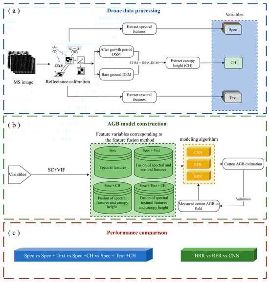
Figure 3. Workflow diagram. (a) UAV data processing workflow. (b) AGB estimation model construction. (c) Performance comparison.

3. Results

3.1. Temporal Dynamics of Cotton Canopy Characteristics Derived from UAV Multispectral Data

3.1.1. Visual Changes in Multi-Temporal UAV Multispectral Imagery

The UAV false color (NIR–R–G) images clearly reveal the temporal dynamics of cotton growth across the five stages (Figure 4). At the seedling stage, vegetation signals were weak and discontinuous, indicating low canopy cover and limited biomass. At the squaring stage, the canopy rapidly expanded with enhanced NIR reflectance and reduced soil exposure. The flowering stage exhibited the strongest and most uniform red tones, corresponding to canopy closure, maximal LAI, and vigorous biomass accumulation. During the boll setting stage, the canopy structure became more complex and slightly heterogeneous due to boll formation. By the boll opening stage, NIR reflectance decreased, and canopy fragmentation increased, reflecting leaf senescence and reduced vegetation vigor. Overall, the false color images effectively captured canopy cover, vigor, and structural changes throughout the cotton growth cycle.

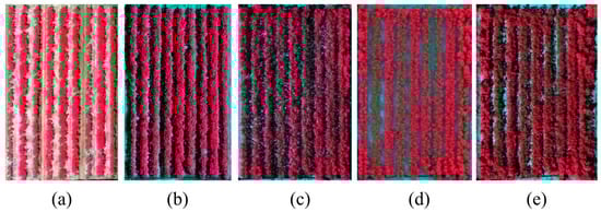
Figure 4. UAV false color images of a representative cotton plot acquired at the cotton growth stage. (a) Seedling stage, (b) squaring stage, (c) flowering stage, (d) boll setting stage, and (e) boll opening stage.

3.1.2. Temporal Variation in Spectral, Textural Features and CHM

For temporal feature visualization, we selected NDVI as the representative spectral feature due to its strong association with canopy greenness and physiological activity. The entropy from the NIR band (NIR_ENT) captures stage-dependent increases in canopy structural heterogeneity and surface complexity, thereby reflecting the accumulation of cotton aboveground biomass. CHM directly reflects plant height dynamics and biomass accumulation. These three features collectively represent physiological, spatial, and structural aspects of cotton canopy development.

The NDVI exhibited a clear temporal growth pattern across the five cotton stages (Figure 5 and Figure 6). NDVI showed a continuous increase from the seedling to the flowering stage, indicating canopy expansion and enhanced photosynthetic activity. It slightly decreased during the boll setting stage and dropped sharply at the boll opening stage, reflecting canopy thinning and late-season senescence.

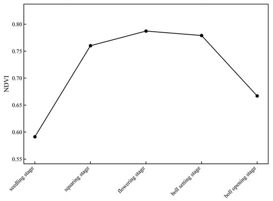
Figure 5. Temporal variation in NDVI across five cotton growth stages.

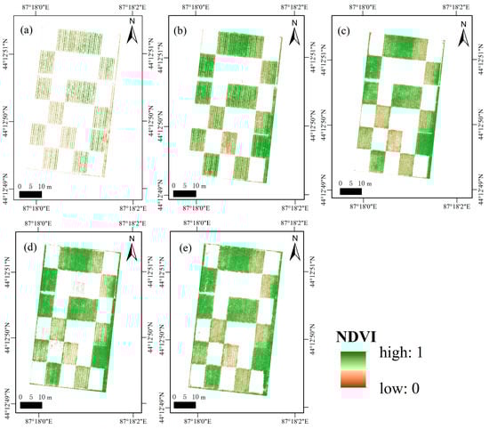
Figure 6. NDVI changes during the 2023 cotton growing season. (a) seedling stage, (b) squaring stage, (c) flowering stage, (d) boll setting stage, and (e) boll opening stage.

The NIR_ENT shows a clear increasing trend from the seedling to boll setting stage, with a slight decrease at boll opening (Figure 7). The raster maps exhibit relatively low and homogeneous entropy values at early growth stages, while progressively higher and more heterogeneous patterns emerge as canopy development advances, indicating increased structural complexity. At the boll opening stage, localized reductions in entropy are observed, associated with leaf senescence and partial canopy fragmentation (Figure 8). This pattern reflects the transition of the cotton canopy from a simple and sparse structure to a dense and complex canopy, and subsequently to a partially fragmented state, thereby indicating the accumulation, stabilization, and late-season variation in cotton aboveground biomass.

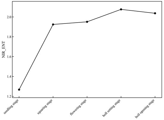
Figure 7. Temporal variation in entropy from the NIR band (NIR_ENT) across cotton growth stages.

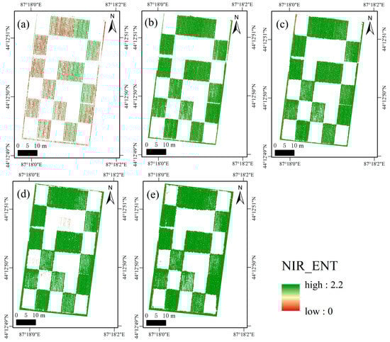
Figure 8. NIR_ENT changes during the 2023 cotton growing season. (a) seedling stage, (b) squaring stage, (c) flowering stage, (d) boll setting stage, and (e) boll opening stage.

The CHM showed a clear and continuous increasing trend from the seedling stage to the boll opening stage, with a particularly rapid increase from the squaring to boll setting stages (Figure 9). The corresponding raster maps reveal a gradual expansion of high canopy height areas and increasing spatial continuity as cotton plants grow taller and the canopy becomes more developed (Figure 10). This pattern reflects the vertical growth dynamics of cotton, indicating progressive plant height increase and structural maturation, which are closely associated with the accumulation of AGB.

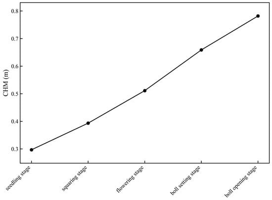
Figure 9. Temporal variation in the canopy height model (CHM) across five cotton growth stages.

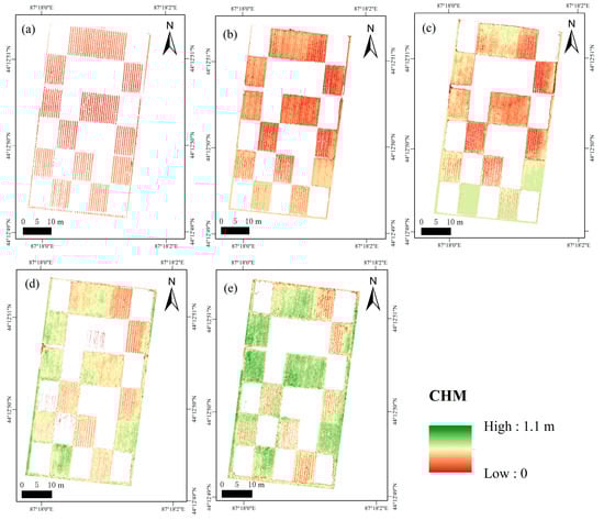
Figure 10. CHM changes during the 2023 cotton growing season. (a) seedling stage, (b) squaring stage, (c) flowering stage, (d) boll setting stage, and (e) boll opening stage.

3.2. Spearman’s Correlation Analysis Between Spectral and Texture Features and Cotton AGB Across Five Growth Stages

Figure 11 shows Spearman’s correlations between spectral features and AGB. Only a few VIs exhibited absolute Spearman’s correlation coefficients ($\left|\mathrm{r}\right|$) greater than 0.8 with cotton AGB. Among these, GNDVI and RVI2 showed the highest $\left|\mathrm{r}\right|$ values, both reaching 0.87 (p < 0.01). The R, G, and B bands maintain moderate correlations with cotton AGB, which can be attributed to their sensitivity to canopy reflectance variations captured by high-resolution UAV imagery. Meanwhile, OSAVI1 is positioned between raw spectral bands and conventional spectral features, indicating its ability to integrate spectral contrast while reducing background effects. This behavior is further strengthened by the prior removal of bare soil pixels using an NDVI threshold, which improves the sensitivity of OSAVI1 to cotton AGB.

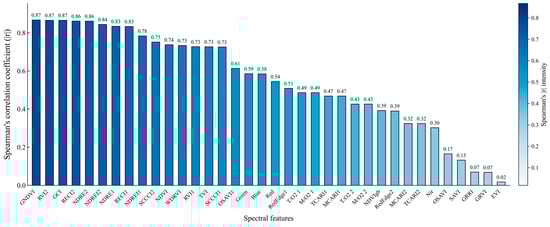
Figure 11. Spearman’s correlation coefficient (|r|) bar chart of spectral features with cotton AGB across entire growth stages. All correlations are statistically significant (p < 0.05).

Figure 12 shows Spearman’s correlations between texture features and AGB. Texture features with cotton AGB Spearman’s correlation coefficient “|r|” greater than 0.7 are relatively rare. Among them, N_ASM and RE2_ASM showed the highest |r| values, both reaching 0.71 (p < 0.01).

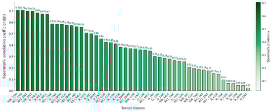
Figure 12. Spearman’s correlation coefficient (|r|) bar chart of textural features with cotton AGB across entire growth stages. All correlations are statistically significant (p < 0.05).

This study selected spectral features and texture features with |r| > 0.6 (p < 0.01). A total of 16 spectral feature variables and 8 texture feature variables were selected.

3.3. Spectral and Texture Feature Selection Based on Variance Inflation Factor (VIF) Across Five Growth Stages of Cotton

Select spectral and texture features with strong correlations through Spearman’s correlation analysis (|r| > 0.6, p < 0.05). To avoid multicollinearity among variables and identify the most effective predictors for cotton AGB, the VIF method is applied to screen the remaining spectral and texture features. For the selected spectral and textural features, repeatedly compute VIF for all features. In each iteration, remove the feature with the highest VIF exceeding the threshold (10) until the VIF of all features falls below the threshold. Table 6 displays the feature indicators used as inputs in the model and their VIF values.

Table 6. Feature indicators for the input model and VIF value.

Feature	Feature Indicators	VIF
Spectral feature	WDRVI	1.33
	TVI	6.19
	OSAVI1	6.30
Textural feature	NIR_ASM	2.05
	NIR_ENT	2.05
Canopy height	CHM	-

After VIF filtering, OSAVI1 was retained. This selection was not based on maximizing individual correlation strength, but on minimizing redundancy while preserving representative information. Among the collinear spectral feature variables, OSAVI1 exhibited a moderate VIF value (<10) and maintained a strong relationship with cotton aboveground biomass. In contrast, other collinear indices with higher VIF values were excluded due to redundant spectral information and stronger multicollinearity. Therefore, OSAVI1 was retained as a representative and complementary feature for subsequent biomass modeling.

3.4. Temporal Variation in Spearman’s Correlation Correlations Between AGB and Spectral, Texture, and CHM

This study presents the correlation curves over time for the features ultimately used in modeling after undergoing Spearman’s correlation analysis and VIF screening, as these are the features actually employed by the model.

The correlations between spectral features and AGB vary across growth stages, generally strengthening from the seedling to squaring stages, weakening around flowering and partly during boll setting, and increasing again at the boll opening stage, indicating a clear stage dependency relationship with cotton AGB (Figure 13). For WDRVI, Spearman’s correlation with AGB increases from the seedling to squaring stages, drops at the flowering stage, and then rises again during boll setting and boll opening stages, where it reaches the highest values. This suggests that WDRVI is sensitive to canopy densification and late-season biomass accumulation, while its correlation is reduced around flowering, due to spectral saturation or structural changes in the canopy. TVI shows an increase in Spearman’s correlation from the seedling to squaring stages, a marked decrease at the flowering and boll setting stages, and a partial recovery at the boll opening stage, though correlations remain moderate overall. This indicates that TVI can track early to middle season canopy growth to some extent, but its linkage to AGB weakens when canopy structure becomes most complex. OSAVI1 maintains relatively high Spearman’s correlations across all stages, with a slight decrease in flowering but pronounced increases during boll setting and boll opening. This pattern reflects its robustness against soil background and its stable sensitivity to changes in leaf area and canopy photosynthetic capacity, making it a reliable spectral indicator of AGB. Additionally, the soil background interference in OSAVI1 was further reduced by employing the NDVI thresholding method to remove bare ground pixels. Consequently, the correlation between OSAVI1 and AGB across different cotton growth stages became more authentic and stable, with variations primarily driven by canopy physiological and structural evolution rather than masking treatments.

Figure 13. Spearman’s correlation between partial spectral features and cotton AGB at five growth stages. S1: seedling stage; S2: squaring stage; S3: flowering stage; S4: boll setting stage; S5: boll opening stage. * p < 0.05; ** p < 0.01.

Figure 14 shows Spearman’s correlations between the angular second moment (NIR_ASM) and entropy (NIR_ENT) in the NIR band and the AGB at five growth stages of cotton. Spearman’s correlation between NIR_ASM and AGB increases from the seedling to the flowering stage as the canopy becomes denser, decreases slightly at the boll setting stage due to boll development and shadow pattern changes, and rises sharply at the boll opening stage with canopy fragmentation, showing strong sensitivity to increasing heterogeneity. NIR_ENT increases from the seedling to the flowering stage as canopy complexity grows, decreases slightly at the boll setting stage due to texture disturbances from boll distribution, and rises again at the boll opening stage with enhanced canopy fragmentation, indicating strong responsiveness to late-season structural variability.

Figure 14. Spearman’s correlation between partial texture features and cotton AGB at five growth stages. S1: seedling stage; S2: squaring stage; S3: flowering stage; S4: boll setting stage; S5: boll opening stage. * p < 0.05; ** p < 0.01.

Figure 15 shows Spearman’s correlations between the CHM and cotton AGB at five growth stages of cotton. Spearman’s correlation between CHM and AGB is relatively low during the seedling and squaring stages because plant height differences remain small and insufficient to reflect biomass variation. The correlation increases substantially at the flowering stage as rapid vertical growth and canopy expansion enhance the linkage between height and biomass. A decline is observed at the boll setting stage, due to slower height growth and a more stabilized canopy structure, which reduces the sensitivity of CHM to biomass differences. The correlation rises again and reaches its highest level at the boll opening stage, indicating that plant height closely represents biomass accumulation at maturity. Overall, CHM exhibits stronger predictive ability for AGB during mid-to-late growth stages.

Figure 15. Spearman’s correlation between CHM and cotton AGB at five growth stages. S1: seedling stage; S2: squaring stage; S3: flowering stage; S4: boll setting stage; S5: boll opening stage. * p < 0.05; ** p < 0.01.

3.5. Cotton AGB Estimation Model for Five Growth Periods of Cotton

To fully characterize the dynamic growth of cotton, multi-temporal derived features of UAV were incorporated into the AGB estimation model. Features derived from a single acquisition date could only reflect the instantaneous canopy status, but could not represent the overall biomass accumulation trajectory. Therefore, features from all acquisition dates, including spectral, textural features, and CH, were combined into a unified feature set. Based on this multi-temporal feature framework, we further compared different feature fusion methods and evaluated multiple algorithms to determine the optimal approach for cotton AGB estimation.

3.5.1. Comparing Different Image Feature Fusion Methods for Estimating Cotton AGB

The estimation of cotton AGB using four image feature combinations yielded the results summarized in Table 7 and Figure 16 Using spectral features for AGB estimation resulted in R² values of 0.57 to 0.67, RMSE of 0.25 to 0.22 kg·m^−2, and MAE of 0.19 to 0.15 kg·m⁻². This indicates that spectral features can only explain part of the variability in AGB estimation results. Combining spectral and textural features improved R² to 0.58 to 0.74, while RMSE decreased to 0.25 to 0.19 kg·m⁻² and MAE to 0.18 to 0.13 kg·m⁻². This demonstrates that incorporating textural information enhanced the estimation of AGB. Integrating spectral and CH further improved model performance, with R² increasing to 0.71 to 0.78, RMSE decreasing to 0.21 to 0.18 kg·m^−2, and MAE to 0.15 to 0.12 kg·m⁻². These findings suggest that the inclusion of canopy height information substantially enhanced AGB estimation, yielding greater improvement than the spectral and textural fusion. This also indicates that CH contributes more significantly than textural features to the cotton AGB estimation model. The growth of cotton is closely related to its height. The fusion of spectral, textural features, and CH completed the highest overall performance, with R² ranging from 0.72 to 0.80, RMSE reduced to 0.21 to 0.17 kg·m⁻², and MAE to 0.15 to 0.11 kg·m⁻². Compared with the three preceding approaches, this comprehensive fusion provided the most accurate AGB estimates. Overall, these results demonstrate that the integrated spectral, textural features, and CH approach captured the variability of cotton AGB more effectively and produced more accurate estimation results. This highlights how multiple features can effectively compensate for the limitations of single features, providing a more comprehensive reflection of crop growth characteristics.

Table 7. Accuracy statistics for cotton AGB estimation with different feature fusion methods and algorithms.

Image Feature Fusion Method	Norm	Model	Number of Variables	Variable Name	Test Sets
					R2	RMSE (kg·m−2)	MAE (kg·m−2)
Spectral features	Spec	BRR	3	WDRVI, TVI, OSAVI1	0.57	0.25	0.19
		RFR			0.62	0.24	0.16
		CNN			0.67	0.22	0.15
Fusion of spectral and textural features	Spec + Text	BRR	5	WDRVI, TVI, OSAVI1, NIR_ASM, NIR_ENT	0.58	0.25	0.18
		RFR			0.72	0.20	0.15
		CNN			0.74	0.19	0.13
Fusion of spectral features and canopy height	Spec + CH	BRR	4	WDRVI, TVI, OSAVI1, CHM	0.71	0.21	0.15
		RFR			0.77	0.19	0.13
		CNN			0.78	0.18	0.12
Fusion of spectral, textural features and canopy height	Spec + Text + CH	BRR	6	WDRVI, TVI, OSAVI1, NIR_ASM, NIR_ENT, CHM	0.72	0.21	0.15
		RFR			0.78	0.18	0.12
		CNN			0.80	0.17	0.11

Figure 16. Comparison of different image feature fusion methods in cotton AGB estimate accuracy. (a) R², (b) RMSE, (c) MAE.

The predicted AGB values from each fold of the test set are aggregated to obtain AGB predictions for all samples across all cotton growth stages. These AGB predicted values and their corresponding actual AGB values generate a scatter plot for the test set. A comparative analysis of scatter plots estimating cotton AGB using four feature fusion methods is presented in Figure 17. Compared to other feature fusion approaches, the scatter plot combining spectral, textural features, and CH exhibits tighter clustering of points around the 1:1 line, indicating stronger and more consistent correlation with AGB measurements. The combined use of spectral, textural, and CH features enables the model to capture more spectral, textural, and structural information, thereby achieving more accurate and stable estimates for cotton. This demonstrates that multi-feature fusion provides a more comprehensive understanding of factors influencing cotton AGB, offering superior estimation performance compared to other feature fusion methods.

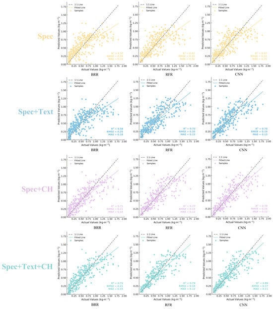
Figure 17. Scatter diagram of AGB predicted values and actual values based on four feature fusion methods (Spec, Spec + Text, Spec + CH, Spec + Text + CH) and three algorithms (BRR, RFR, CNN).

3.5.2. Comparison of Different Algorithms for Estimating Cotton AGB

Table 7 and Figure 18 show the performance of three algorithms used to estimate AGB. The results show a consistent ranking of estimation accuracy from lowest to highest as BRR < RFR < CNN. It becomes clear that although the combinations of input image features affect the accuracy of AGB estimation, the CNN model consistently performs more accurately than RFR and BRR. CNN demonstrates significant advantages in spatial data processing, effectively extracting complex nonlinear relationships and interactions between features to achieve higher estimation accuracy.

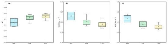
Figure 18. Comparison of different algorithms in cotton AGB estimate accuracy. (a) R2, (b) RMSE, (c) MAE.

3.5.3. Optimal Strategy for Estimating Cotton AGB via Integration of Image-Feature Fusion Approaches and Models

Even after controlling for multicollinearity via VIF, nonlinear models such as RFR and CNN outperformed the linear model BRR in AGB fitting, indicating their superior ability to capture nonlinear dependencies. When confronted with complex multiple feature variables, the CNN model demonstrated superior capability in estimating cotton AGB (R² = 0.80; RMSE = 0.17 kg·m⁻²; MAE = 0.11 kg·m⁻²). The accuracy of estimating cotton AGB through fused spectral, textural features, and CH also surpasses that achieved by using spectral features alone, spectral and textural features combined.

3.6. Performance of Cotton AGB Prediction at Different Cotton Growth Stages

To investigate the model performance at different cotton growth stages, the predicted and measured AGB values from the test sets of the five-fold cross-validation were further grouped according to growth stages. For each growth stage, R², RMSE, and MAE were calculated based on the corresponding test samples.

The model exhibited distinct performance variations across different cotton growth stages (Table 8). Higher prediction accuracy was achieved at the boll opening stages, with an R² of 0.49, RMSE of 0.27 kg·m⁻², and MAE of 0.21 kg·m⁻². The R² value during the cotton seedling stage was negative. This indicates that the prediction error during the seedling stage exceeds the variance of the measured AGB around its mean. This is mainly due to the extremely low biomass level and limited variability at the seedling stage. Under such conditions, even small prediction errors can lead to a disproportionately large reduction in R². In addition, sparse canopy cover and strong soil background effects during early growth stages reduce the sensitivity of derived features of UAV to AGB, thereby limiting prediction accuracy.

Table 8. Accuracy statistics for cotton AGB estimation across different growth stages.

Image Feature Fusion Method	Norm	Variable Name	Model	Growing Stage of Cotton	Test Sets
					R2	RMSE (kg·m−2)	MAE (kg·m−2)
Fusion of spectral, textural, and canopy height (CH)	Spec + Text + CH	WDRVI, TVI, OSAVI1, NIR_ASM, NIR_ENT, CHM	CNN	seedling stage	−1.72	0.04	0.03
				squaring stage	0.27	0.08	0.06
				flowering stage	0.10	0.16	0.12
				boll setting stage	0.35	0.22	0.16
				boll opening stage	0.49	0.27	0.21

4. Discussion

4.1. Insights into the Role of Multi-Feature Fusion for AGB Estimation

This study investigates the effectiveness of multi-feature fusion from UAV in estimating cotto AGB. These findings suggest that integrating spectral, textural features, and CH significantly improves the accuracy of cotton AGB estimation, outperforming methods relying solely on spectral features, the combination of spectral and textural features, and the integration of spectral features and canopy height. Early studies predominantly employed spectral features to estimate crop AGB. For instance, Wang et al. [11] utilized spectral features from MS drone imagery to estimate the aboveground biomass of winter wheat. However, as canopy density increases, spectral reflectance becomes saturated, reducing its sensitivity to changes in biomass. In contrast, by integrating textural features and CH, this approach provides both surface and vertical structural information of the canopy. This overcomes the limitation of easy saturation of spectral features, thereby enhancing the accuracy of AGB estimation. This aligns with recent research findings, such as those reported by Yue et al. [71], who demonstrated that the integration of spectral and textural features significantly improved estimates of wheat AGB. Similarly, Herrero-Huerta et al. [72] demonstrated that integrating spectral and canopy height can enhance the predictive performance of soybean AGB. The findings of this study further support these conclusions, as both fusion strategies improved cotton AGB estimation precision. Textural features describe the statistical characteristics of pixel gray level distribution under given spatial relationships, such as contrast and homogeneity [73]. They capture the spatial distribution and structural variations in crops, including leaf arrangement and canopy density. Furthermore, the spatial structure of crops exhibits distinct three-dimensional features, manifesting not only in horizontal distribution but also in vertical stratification. CH, as a key structural characteristic, is closely related to the vertical structure of crops [74]. Moreover, the integration of spectral, textural, and CH produced the highest estimation precision. Sun et al. [75] also demonstrated this by estimating the AGB of rapeseed at different growth stages using spectral, textural features, and CH, achieving good estimation accuracy. By integrating spectral features, textural features, and CH, it is possible to more comprehensively reflect crop growth and biomass accumulation processes, thereby achieving stable and highly accurate AGB predictions.

4.2. Advantages of CNN for AGB Estimation

Research has shown that selecting appropriate and efficient algorithms is critical for improving the accuracy of AGB estimation. This study compared the performance of two machine learning algorithms, BRR and RFR, and one deep learning algorithm, CNN, in estimating cotton AGB. The results indicate that CNN achieved higher estimation accuracy than both RFR and BRR, particularly when modeling complex data relationships. These findings are consistent with recent research results. These studies demonstrate that deep learning models exhibit good effectiveness in remote sensing tasks. Yu et al. [76] introduced a CNN model for estimating corn aboveground biomass. The results demonstrate that CNN can extract high-dimensional spatial features from UAV imagery and capture the nonlinear relationship between these features and aboveground biomass. Compared to traditional machine learning methods such as multiple linear regression (MLR), RFR, and support vector machine regression (SVR), CNN achieves more robust and accurate biomass estimation results without requiring manual feature extraction. Zu et al. [77] found that CNN can effectively extract coupled features of spatial structure and spectral information in multispectral imagery, better characterizing the nonlinear relationship between winter wheat LAI and remote sensing signals. Their estimation accuracy and stability significantly outperform traditional machine learning methods. Yue et al. [78] demonstrated that CNN outperformed traditional methods such as PLSR, SVR, RFR, and Gaussian Process Regression (GPR) in estimating chlorophyll content in Ginkgo Seedlings. The strength of CNN lies in its capacity to capture intricate nonlinear relationships that enhance model predictive capability. In contrast, RFR improves stability by integrating multiple decision trees to reduce noise interference. However, its performance declines when dealing with high-dimensional features, resulting in slightly lower accuracy than CNN. BRR, as a linear regression method, is limited in its ability to model nonlinear patterns and performs less effectively when applied to complex, high-dimensional datasets.

Overall, the CNN algorithm demonstrates superior performance in AGB estimation due to its strong nonlinear modeling capacity and powerful feature extraction capability, outperforming traditional machine learning approaches in accuracy.

4.3. Study Limitations and Prospects for Future Research

This study still has several limitations. First, the multi-feature fusion strategy (spectral, textural, and canopy height features) was developed and validated using data from a single crop, which may limit its universality. Moreover, the present study is limited by the use of data from a single growing season and field site. While the experimental plots cover a wide range of irrigation levels and canopy growth conditions that provided useful variability for model development, these factors cannot fully substitute for the broader environmental and interannual variability encountered in operational settings. Second, the precision of canopy structural information may constrain the performance of methods that combine spectral features and CH, as well as those that integrate spectral, textural features, and CH. Higher precision CHM measurements should be more widely implemented. Third, although the proposed CNN framework demonstrates stable performance, a lightweight CNN architecture was adopted due to the limited sample size. More complex deep learning models, such as CNN–LSTM or transformer networks, were not explored, as they typically require much larger datasets to train effectively and tend to overfit under small sample conditions. Additionally, this study aimed to explore the ability of deep learning models and traditional machine learning algorithms (RFR and BRR) to capture nonlinear relationships between multiple traits and biomass. Therefore, deep learning models represented by CNN were selected. Finally, although this study evaluated AGB prediction accuracy across different growth stages, we did not establish independent models for each stage. The primary reason is that the sample size of individual stages was relatively limited and unevenly distributed, which may lead to unstable or non-generalizable models if trained separately. In addition, the objective of this study was to develop a unified model capable of predicting AGB across multiple stages rather than comparing specific stage models.

Multi-feature fusion and framework based on CNN achieved promising performance. Future research should extend this framework to multi-year datasets, diverse geographic regions, and multiple crops (e.g., maize, wheat, and rice), in order to more comprehensively evaluate its robustness, transferability, and generalizability. Meanwhile, Higher precision CHM measurements can improve the accuracy of AGB estimates. We consider that the preference should be given to using LiDAR sensors to further improve mapping accuracy, while also incorporating other plant structural features to enhance biomass estimation. Future research could investigate advanced deep architectures. In terms of algorithms, future work can extend to larger datasets and explore advanced deep learning architectures, such as CNN–LSTM and transformer networks. Regarding modeling at different growth stages, future research could further explore traits for biomass at each developmental phase and determine which stage best predicts cotton biomass performance. Furthermore, leveraging the advantages of multi-feature fusion techniques, future research could involve integrating multiple sensors (e.g., hyperspectral and temperature sensors) in order to extract additional features from imagery, thereby further improving estimation accuracy.

4.4. Main Contributions of the Research

From a theoretical perspective, the primary contribution of this study lies in proposing a novel approach for estimating crop AGB using UAV remote sensing. By integrating spectral, textural features, and CH with a CNN framework, the method effectively addresses the challenges of canopy spectral saturation and multiple feature redundancy. The integration of multiple features with deep learning not only enhances the precision of cotton AGB estimation but also serves as a methodological reference for constructing AGB estimation models based on UAV for other crops.

From an application perspective, this study enhances the accuracy of crop AGB estimation by integrating multiple features with deep learning models. This improvement provides more reliable technical support for crop growth monitoring and farmland management based on UAV remote sensing. The integration of spectral, textural features, and CH enables more reliable assessments of canopy vigor, structural uniformity, and biomass accumulation, providing agronomically meaningful indicators for in-season management. Beyond improving model performance, this research establishes a methodological framework for field-scale crop monitoring based on UAV remote sensing, which supports farmland decision-making and management practices. Moreover, the proposed framework can be extended to other crops and target variables, such as nitrogen status and yield prediction.

5. Conclusions

This study utilized multispectral imagery from UAV to extract spectral, textural features, and CH. By integrating these multiple features with machine learning algorithms, an estimation model for AGB in cotton was developed. The research systematically investigated the impact of image feature fusion and model algorithms on AGB estimation accuracy, seeking optimal joint strategies. Key findings are as follows:

• The fusion of spectral, textural features, and CH outperforms single spectral features, spectral and texture features fusion, and spectral features and CH fusion. The method integrating spectral, textural features, and CH achieved the highest estimation precision in this study, indicating that combining multiple feature information may more comprehensively reflect the spatial variation in aboveground biomass.
• Deep learning algorithms outperformed traditional methods. In this study, a CNN yielded superior AGB estimates compared to traditional machine learning algorithms like BRR and RFR, demonstrating their advantage in handling complex nonlinear relationships between multiple remote sensing features and AGB.
• The “multiple feature fusion and CNN” strategy yielded the best performance under the study conditions. Integrating spectral, textural features, and CH with the CNN algorithm for estimating cotton AGB demonstrated best performance (R² = 0.80, RMSE = 0.17 kg·m^−2, and MAE = 0.11 kg·m⁻²), indicating its potential applicability under the current experimental setup and providing a reference technical approach for biomass estimation in agricultural remote sensing.

References

- Huang, Y.; Brand, H.J.; Sui, R.; Thomson, S.J.; Furukawa, T.; Ebelhar, M.W. Cotton Yield Estimation Using Very High-Resolution Digital Images Acquired with a Low-Cost Small Unmanned Aerial Vehicle. Trans. ASABE 2016, 59, 1563–1574. [Google Scholar]
- Zhang, J.; Fang, H.; Zhou, H.; Sanogo, S.; Ma, Z. Genetics, Breeding, and Marker-Assisted Selection for Verticillium Wilt Resistance in Cotton. Crop Sci. 2014, 54, 1289–1303. [Google Scholar] [CrossRef]
- Li, B.; Xu, X.; Zhang, L.; Han, J.; Bian, C.; Li, G.; Liu, J.; Jin, L. Above-Ground Biomass Estimation and Yield Prediction in Potato by Using UAV-Based RGB and Hyperspectral Imaging. ISPRS J. Photogramm. Remote Sens. 2020, 162, 161–172. [Google Scholar] [CrossRef]
- Virk, G.; Adhikari, B.N.; Hinze, L.L.; Hequet, E.F.; Stelly, D.M.; Kelly, C.M.; Hague, S.; Percy, R.G.; Dever, J.K. Physiological Contributors to Yield in Advanced Cotton Breeding Lines. Crop Sci. 2023, 63, 3264–3276. [Google Scholar] [CrossRef]
- Khan, A.; Kong, X.; Najeeb, U.; Zheng, J.; Tan, D.K.Y.; Akhtar, K.; Munsif, F.; Zhou, R. Planting Density Induced Changes in Cotton Biomass Yield, Fiber Quality, and Phosphorus Distribution under Beta Growth Model. Agronomy 2019, 9, 500. [Google Scholar] [CrossRef]
- Aierken, N.; Yang, B.; Li, Y.; Jiang, P.; Pan, G.; Li, S. A Review of Unmanned Aerial Vehicle–Based Remote Sensing and Machine Learning for Cotton Crop Growth Monitoring. Comput. Electron. Agric. 2024, 227, 109601. [Google Scholar] [CrossRef]
- Yang, S.; Feng, Q.; Liang, T.; Liu, B.; Zhang, W. Modeling Grassland Above-Ground Biomass Based on Artificial Neural Network and Remote Sensing in the Three-River Headwaters Region. Remote Sens. Environ. 2018, 204, 448–455. [Google Scholar] [CrossRef]
- Yue, J.; Yang, G.; Li, C.; Li, Z.; Wang, Y.; Feng, H.; Xu, B. Estimation of Winter Wheat Above-Ground Biomass Using Unmanned Aerial Vehicle-Based Snapshot Hyperspectral Sensor and Crop Height Improved Models. Remote Sens. 2017, 9, 708. [Google Scholar] [CrossRef]
- Wang, T.; Liu, Y.; Wang, M.; Fan, Q.; Tian, H.; Qiao, X.; Li, Y. Applications of UAS in Crop Biomass Monitoring: A Review. Front. Plant Sci. 2021, 12, 616689. [Google Scholar] [CrossRef]
- Zhang, S.; Wang, X.; Lin, H.; Dong, Y.; Qiang, Z. A Review of the Application of UAV Multispectral Remote Sensing Technology in Precision Agriculture. Smart Agric. Technol. 2025, 12, 101406. [Google Scholar] [CrossRef]
- Wang, F.; Yang, M.; Ma, L.; Zhang, T.; Qin, W.; Li, W.; Zhang, Y.; Sun, Z.; Wang, Z.; Li, F.; et al. Estimation of Above-Ground Biomass of Winter Wheat Based on Consumer-Grade Multi-Spectral UAV. Remote Sens. 2022, 14, 1251. [Google Scholar] [CrossRef]
- Liu, Y.; Liu, S.; Li, J.; Guo, X.; Wang, S.; Lu, J. Estimating Biomass of Winter Oilseed Rape Using Vegetation Indices and Texture Metrics Derived from UAV Multispectral Images. Comput. Electron. Agric. 2019, 166, 105026. [Google Scholar] [CrossRef]
- Chen, P.; Wang, F. New Textural Indicators for Assessing Above-Ground Cotton Biomass Extracted from Optical Imagery Obtained via Unmanned Aerial Vehicle. Remote Sens. 2020, 12, 4170. [Google Scholar] [CrossRef]
- Chen, M.; Yin, C.; Lin, T.; Liu, H.; Wang, Z.; Jiang, P.; Ali, S.; Tang, Q.; Jin, X. Integration of Unmanned Aerial Vehicle Spectral and Textural Features for Accurate Above-Ground Biomass Estimation in Cotton. Agronomy 2024, 14, 1313. [Google Scholar] [CrossRef]
- Liu, Y.; Feng, H.; Yue, J.; Jin, X.; Li, Z.; Yang, G. Estimation of Potato Above-Ground Biomass Based on Unmanned Aerial Vehicle Red–Green–Blue Images with Different Texture Features and Crop Height. Front. Plant Sci. 2022, 13, 938216. [Google Scholar] [CrossRef]
- Liu, J.; Zhu, Y.; Song, L.; Su, X.; Li, J.; Zheng, J.; Zhu, X.; Ren, L.; Wang, W.; Li, X. Optimizing Window Size and Directional Parameters of GLCM Texture Features for Estimating Rice AGB Based on UAVs Multispectral Imagery. Front. Plant Sci. 2023, 14, 1284235. [Google Scholar] [CrossRef]
- Zubair, A.R.; Alo, O.A. Grey Level Co-Occurrence Matrix (GLCM) Based Second Order Statistics for Image Texture Analysis. arXiv 2024, arXiv:2403.04038. [Google Scholar] [CrossRef]
- Liu, H.; Dong, P. A New Method for Generating Canopy Height Models from Discrete-Return LiDAR Point Clouds. Remote Sens. Lett. 2014, 5, 575–582. [Google Scholar] [CrossRef]
- Valluvan, A.B.; Raj, R.; Pingale, R.; Jagarlapudi, A. Canopy Height Estimation Using Drone-Based RGB Images. Smart Agric. Technol. 2023, 4, 100145. [Google Scholar] [CrossRef]
- Maimaitijiang, M.; Chang, J.; Caffe, M. Utilizing Spectral, Structural and Textural Features for Estimating Oat Above-Ground Biomass Using UAV-Based Multispectral Data and Machine Learning. Sensors 2023, 23, 9708. [Google Scholar]
- Luo, S.; Jiang, X.; He, Y.; Li, J.; Jiao, W.; Zhang, S.; Xu, F.; Han, Z.; Sun, J.; Yang, J.; et al. Multi-Dimensional Variables and Feature Parameter Selection for Aboveground Biomass Estimation of Potato Based on UAV Multispectral Imagery. Front. Plant Sci. 2022, 13, 948249. [Google Scholar] [CrossRef] [PubMed]
- Li, M.; Wang, W.; Li, H.; Yang, Z.; Li, J. Monitoring of Vegetation Chlorophyll Content in Photovoltaic Areas Using UAV-Mounted Multispectral Imaging. Front. Plant Sci. 2025, 16, 1643945. [Google Scholar] [CrossRef]
- Grüner, E.; Wachendorf, M.; Astor, T. The Potential of UAV-Borne Spectral and Textural Information for Predicting Aboveground Biomass and N Fixation in Legume–Grass Mixtures. PLoS ONE 2020, 15, e0234703. [Google Scholar] [CrossRef]
- Xu, T.; Wang, F.; Xie, L.; Yao, X.; Zheng, J.; Li, J.; Chen, S. Integrating the Textural and Spectral Information of UAV Hyperspectral Images for the Improved Estimation of Rice Aboveground Biomass. Remote Sens. 2022, 14, 2534. [Google Scholar] [CrossRef]
- Zou, M.; Liu, Y.; Fu, M.; Li, C.; Zhou, Z.; Meng, H.; Xing, E.; Ren, Y. Combining Spectral and Texture Feature of UAV Image with Plant Height to Improve LAI Estimation of Winter Wheat at Jointing Stage. Front. Plant Sci. 2024, 14, 1272049. [Google Scholar] [CrossRef]
- Lv, Z.; Meng, R.; Man, J.; Zeng, L.; Wang, M.; Xu, B.; Gao, R.; Sun, R.; Zhao, F. Modeling of Winter Wheat fAPAR by Integrating Unmanned Aircraft Vehicle-Based Optical, Structural and Thermal Measurement. Int. J. Appl. Earth Obs. Geoinf. 2021, 102, 102407. [Google Scholar] [CrossRef]
- Yin, Q.; Yu, X.; Li, Z.; Du, Y.; Ai, Z.; Qian, L.; Huo, X.; Fan, K.; Wang, W.; Hu, X. Estimating Summer Maize Biomass by Integrating UAV Multispectral Imagery with Crop Physiological Parameters. Plants 2024, 13, 3070. [Google Scholar] [CrossRef]
- Astor, T.; Dayananda, S.; Nautiyal, S.; Wachendorf, M. Vegetable Crop Biomass Estimation Using Hyperspectral and RGB 3D UAV Data. Agronomy 2020, 10, 1600. [Google Scholar] [CrossRef]
- Hunt, M.L.; Blackburn, G.A.; Carrasco, L.; Redhead, J.W.; Rowland, C.S. High-Resolution Wheat Yield Mapping Using Sentinel-2. Remote Sens. Environ. 2019, 233, 111410. [Google Scholar] [CrossRef]
- Qi, H. Monitoring of Peanut Leaves Chlorophyll Content Based on Drone-Based Multispectral Image Feature Extraction. Comput. Electron. Agric. 2021, 187, 106292. [Google Scholar] [CrossRef]
- Zhang, L.; Han, W.; Niu, Y.; Chávez, J.L.; Shao, G.; Zhang, H. Evaluating the Sensitivity of Water-Stressed Maize Chlorophyll and Structure Based on UAV-Derived Vegetation Indices. Comput. Electron. Agric. 2021, 185, 106174. [Google Scholar] [CrossRef]
- MacKay, D.J.C. Bayesian Interpolation. Neural Comput. 1992, 4, 415–447. [Google Scholar] [CrossRef]
- Breiman, L. Random Forests. Mach. Learn. 2001, 45, 5–32. [Google Scholar] [CrossRef]
- Aghdam, H.H.; Heravi, E.J. Guide to Convolutional Neural Networks; Springer: Cham, Switzerland, 2017. [Google Scholar]
- Agbona, A.; Teare, B.; Ruiz-Guzman, H.; Dobreva, I.D.; Everett, M.E.; Adams, T.; Montesinos-Lopez, O.A.; Kulakow, P.A.; Hays, D.B. Prediction of Root Biomass in Cassava Based on Ground Penetrating Radar Phenomics. Remote Sens. 2021, 13, 4908. [Google Scholar] [CrossRef]
- Johansen, K.; Morton, M.J.L.; Malbeteau, Y.; Aragon, B.; Al-Mashharawi, S.; Ziliani, M.G.; Angel, Y.; Fiene, G.; Negrão, S.; Mousa, M.A.A.; et al. Predicting Biomass and Yield in a Tomato Phenotyping Experiment Using UAV Imagery and Random Forest. Front. Artif. Intell. 2020, 3, 28. [Google Scholar] [CrossRef]
- Vawda, M.I.; Lottering, R.; Mutanga, O.; Peerbhay, K.; Sibanda, M. Comparing the Utility of Artificial Neural Networks (ANN) and Convolutional Neural Networks (CNN) on Sentinel-2 MSI to Estimate Dry Season Aboveground Grass Biomass. Sustainability 2024, 16, 1051. [Google Scholar] [CrossRef]
- Gitelson, A.A.; Gritz, Y.; Merzlyak, M.N. Relationships between Leaf Chlorophyll Content and Spectral Reflectance and Algorithms for Non-Destructive Chlorophyll Assessment in Higher Plant Leaves. J. Plant Physiol. 2003, 160, 271–282. [Google Scholar] [CrossRef]
- Wang, Q.; Adiku, S.; Tenhunen, J.; Granier, A. On the Relationship of NDVI with Leaf Area Index in a Deciduous Forest Site. Remote Sens. Environ. 2005, 94, 244–255. [Google Scholar] [CrossRef]
- Romano, E.; Brambilla, M.; Chianucci, F.; Tattoni, C.; Puletti, N.; Chirici, G.; Travaglini, D.; Giannetti, F. Estimating Canopy and Stand Structure in Hybrid Poplar Plantations from Multispectral UAV Imagery. Ann. For. Res. 2024, 67, 143–154. [Google Scholar] [CrossRef]
- Xie, T.; Li, J.; Yang, C.; Jiang, Z.; Chen, Y.; Guo, L.; Zhang, J. Crop Height Estimation Based on UAV Images. Comput. Electron. Agric. 2021, 185, 106155. [Google Scholar] [CrossRef]
- China Meteorological Data Service Center. China Surface Climate Daily Data Set (V3.0). China Meteorological Administration: Beijing. Available online: http://data.cma.cn (accessed on 30 November 2025).
- Zhang, Y.; Liu, X.; Sun, W.; You, T.; Qi, X. Multi-Threshold Remote Sensing Image Segmentation Based on Improved Black-Winged Kite Algorithm. Biomimetics 2025, 10, 331. [Google Scholar] [CrossRef]
- Rouse, J.W., Jr.; Haas, R.H.; Schell, J.A.; Deering, D.W. Monitoring Vegetation Systems in the Great Plains with ERTS; NASA Special Publication SP-351; NASA: Washington, DC, USA, 1974; Volume 1. [Google Scholar]
- Wang, F.M.; Huang, J.F.; Tang, Y.L.; Wang, X.Z. New Vegetation Index and Its Application in Estimating Leaf Area Index of Rice. Rice Sci. 2007, 14, 195–203. [Google Scholar] [CrossRef]
- Broge, N.H.; Leblanc, E. Comparing Prediction Power and Stability of Broadband and Hyperspectral Vegetation Indices for Estimation of Green Leaf Area Index and Canopy Chlorophyll Density. Remote Sens. Environ. 2001, 76, 156–172. [Google Scholar] [CrossRef]
- Rondeaux, G.; Steven, M.; Baret, F. Optimization of Soil-Adjusted Vegetation Indices. Remote Sens. Environ. 1996, 55, 95–107. [Google Scholar] [CrossRef]
- Huete, A.R. A Soil-Adjusted Vegetation Index (SAVI). Remote Sens. Environ. 1988, 25, 295–309. [Google Scholar] [CrossRef]
- Mishra, S.; Mishra, D.R. Normalized Difference Chlorophyll Index: A Novel Model for Remote Estimation of Chlorophyll-a Concentration in Turbid Productive Waters. Remote Sens. Environ. 2012, 117, 394–406. [Google Scholar] [CrossRef]
- Xue, L.; Cao, W.; Luo, W.; Dai, T.; Yan, Z.J. Monitoring Leaf Nitrogen Status in Rice with Canopy Spectral Reflectance. Agron. J. 2004, 96, 135–142. [Google Scholar] [CrossRef]
- Huete, A.; Didan, K.; Miura, T.; Rodriguez, E.P.; Gao, X.; Ferreira, L.G. Overview of the Radiometric and Biophysical Performance of the MODIS Vegetation Indices. Remote Sens. Environ. 2002, 83, 195–213. [Google Scholar] [CrossRef]
- Gitelson, A.; Viña, A.; Ciganda, V. Remote Estimation of Canopy Chlorophyll Content in Crops. Geophys. Res. Lett. 2005, 32, L08403. [Google Scholar] [CrossRef]
- Tucker, C.J. Red and Photographic Infrared Linear Combinations for Monitoring Vegetation. Remote Sens. Environ. 1979, 8, 127–150. [Google Scholar] [CrossRef]
- Verrelst, J.; Schaepman, M.E.; Koetz, B.; Kneubühler, M. Angular Sensitivity Analysis of Vegetation Indices Derived from CHRIS/PROBA Data. Remote Sens. Environ. 2008, 112, 2341–2353. [Google Scholar] [CrossRef]
- Gitelson, A.A.; Merzlyak, M.N. Remote Estimation of Chlorophyll Content in Higher Plant Leaves. Int. J. Remote Sens. 1997, 18, 2691–2697. [Google Scholar] [CrossRef]
- Hassan, M.A.; Yang, M.; Rasheed, A.; Jin, X.; Xia, X.; Xiao, Y.; He, Z. Time-Series Multispectral Indices from Unmanned Aerial Vehicle Imagery Reveal Senescence Rate in Bread Wheat. Remote Sens. 2018, 10, 809. [Google Scholar] [CrossRef]
- Raper, T.B.; Varco, J.J. Canopy-Scale Wavelength and Vegetative Index Sensitivities to Cotton Growth Parameters and Nitrogen Status. Precis. Agric. 2015, 16, 62–76. [Google Scholar] [CrossRef]
- Haboudane, D.; Miller, J.R.; Tremblay, N.; Zarco-Tejada, P.J.; Dextraze, L. Integrated Narrow-Band Vegetation Indices for Prediction of Crop Chlorophyll Content for Application to Precision Agriculture. Remote Sens. Environ. 2002, 81, 416–426. [Google Scholar] [CrossRef]
- Daughtry, C.S.T.; Walthall, C.L.; Kim, M.S.; de Colstoun, E.B.; McMurtrey, J.E., III. Estimating Corn Leaf Chlorophyll Concentration from Leaf and Canopy Reflectance. Remote Sens. Environ. 2000, 74, 229–239. [Google Scholar] [CrossRef]
- Gamon, J.A.; Surfus, J.S. Assessing Leaf Pigment Content with a Reflectometer. New Phytol. 1999, 143, 105–117. [Google Scholar] [CrossRef]
- Hall-Beyer, M. Practical Guidelines for Choosing GLCM Textures to Use in Landscape Classification Tasks over a Range of Moderate Spatial Scales. Int. J. Remote Sens. 2017, 38, 1312–1338. [Google Scholar] [CrossRef]
- Earth Lab. Canopy Height Models, Digital Surface Models & Digital Elevation Models. Earth Data Science, University of Colorado Boulder. Available online: https://earthdatascience.org/courses/use-data-open-source-python/data-stories/what-is-lidar-data/lidar-chm-dem-dsm/ (accessed on 26 October 2025).
- Samadzadegan, F.; Toosi, A.; Dadrass Javan, F. A Critical Review on Multi-Sensor and Multi-Platform Remote Sensing Data Fusion Approaches: Current Status and Prospects. Int. J. Remote Sens. 2025, 46, 1327–1402. [Google Scholar] [CrossRef]
- Cai, T.; Chang, C.; Zhao, Y.; Wang, X.; Yang, J.; Dou, P.; Otgonbayar, M.; Zhang, G.; Zeng, Y.; Wang, J. Within-Season Estimates of 10 m Aboveground Biomass Based on Landsat, Sentinel-2 and PlanetScope Data. Sci. Data 2024, 11, 1276. [Google Scholar] [CrossRef]
- Sedgwick, P. Spearman’s Rank Correlation Coefficient. BMJ 2014, 349, g7327. [Google Scholar] [CrossRef] [PubMed]
- Montgomery, D.C.; Peck, E.A.; Vining, G.G. Introduction to Linear Regression Analysis, 5th ed.; John Wiley & Sons: Hoboken, NJ, USA, 2012. [Google Scholar]
- LeCun, Y.; Bengio, Y.; Hinton, G. Deep Learning. Nature 2015, 521, 436–444. [Google Scholar] [CrossRef]
- Montesinos-López, A.; Montesinos-López, O.A.; de los Campos, G.; Crossa, J.; Burgueño, J.; Luna-Vázquez, F.J. Bayesian Functional Regression as an Alternative Statistical Analysis of High-Throughput Phenotyping Data of Modern Agriculture. Plant Methods 2018, 14, 46. [Google Scholar] [CrossRef]
- Jayathunga, S.; Owari, T.; Tsuyuki, S. Digital Aerial Photogrammetry for Uneven-Aged Forest Management: Assessing the Potential to Reconstruct Canopy Structure and Estimate Living Biomass. Remote Sens. 2019, 11, 338. [Google Scholar] [CrossRef]
- Jin, X.; Li, Z.; Feng, H.; Ren, Z.; Li, S. Deep Neural Network Algorithm for Estimating Maize Biomass Based on Simulated Sentinel-2A Vegetation Indices and Leaf Area Index. Crop J. 2020, 8, 87–97. [Google Scholar] [CrossRef]
- Yue, J.; Yang, G.; Tian, Q.; Feng, H.; Xu, K.; Zhou, C. Estimate of Winter-Wheat above-Ground Biomass Based on UAV Ultrahigh Ground-Resolution Image Textures and Vegetation Indices. ISPRS J. Photogramm. Remote Sens. 2019, 150, 226–244. [Google Scholar] [CrossRef]
- Herrero-Huerta, M.; Gonzalez-Aguilera, D.; Rodriguez-Gonzalvez, P.; Hernandez-Lopez, D.; Fernandez-Hernandez, J.; Turias, I.; Boyko, A.; Lindenbergh, R.; Di Stefano, F. Canopy Roughness: A New Phenotypic Trait to Estimate Biomass. Plant Phenomics 2020, 2020, 6735967. [Google Scholar] [CrossRef]
- Haralick, R.M.; Shanmugam, K.; Dinstein, I. Textural Features for Image Classification. IEEE Trans. Syst. Man, Cybern. 1973, SMC-3, 610–621. [Google Scholar] [CrossRef]
- Kümmerer, R.; Noack, P.O.; Bauer, B. Using High-Resolution UAV Imaging to Measure Canopy Height of Diverse Cover Crops and Predict Biomass. Remote Sens. 2023, 15, 1520. [Google Scholar] [CrossRef]
- Sun, C.; Zhang, W.; Zhao, G.; Wu, Q.; Liang, W.; Ren, N.; Cao, H.; Zou, L. Mapping Rapeseed (Brassica napus L.) Aboveground Biomass in Different Periods Using Optical and Phenotypic Metrics Derived from UAV Hyperspectral and RGB Imagery. Front. Plant Sci. 2024, 15, 1504119. [Google Scholar] [CrossRef]
- Yu, D.; Zha, Y.; Sun, Z.; Li, J.; Jin, X.; Zhu, W.; Bian, J.; Ma, L.; Zeng, Y.; Su, Z. Deep Convolutional Neural Networks for Estimating Maize Above-Ground Biomass Using Multi-Source UAV Images: A Comparison with Traditional Machine Learning Algorithms. Precis. Agric. 2023, 24, 92–113. [Google Scholar] [CrossRef]
- Zu, J.; Yang, H.; Wang, J.; Cai, W.; Yang, Y. Inversion of Winter Wheat Leaf Area Index from UAV Multispectral Images: Classical vs. Deep Learning Approaches. Front. Plant Sci. 2024, 15, 1367828. [Google Scholar] [CrossRef] [PubMed]
- Yue, Z.; Zhang, Q.; Zhu, X.; Zhou, K. Chlorophyll Content Estimation of Ginkgo Seedlings Based on Deep Learning and Hyperspectral Imagery. Forests 2024, 15, 2010. [Google Scholar] [CrossRef]
Disclaimer/Publisher’s Note: The statements, opinions and data contained in all publications are solely those of the individual author(s) and contributor(s) and not of MDPI and/or the editor(s). MDPI and/or the editor(s) disclaim responsibility for any injury to people or property resulting from any ideas, methods, instructions or products referred to in the content. |
© 2025 by the authors. Licensee MDPI, Basel, Switzerland. This article is an open access article distributed under the terms and conditions of the Creative Commons Attribution (CC BY) license.