Machine Learning-Based Prediction of Soil Bulk Density Using Soil Penetration Resistance and Moisture

Abstract

Soil bulk density (BD) is a critical indicator for evaluating soil physical properties and compaction levels. However, the traditional core method is labor-intensive, time-consuming, and destructive. Given the significant positive correlation between BD and soil penetration resistance (PR), and the crucial influence of gravimetric water content (GW), this study investigated the potential of using PR and GW data to predict BD. We integrated datasets from three representative study sites in China and Brazil, covering diverse soil texture types (sandy loam, clay loam, and clay), and employed two traditional empirical models (Multiple Linear Regression (MLR) and Multiple Nonlinear Regression (MNLR)) and three advanced machine learning (ML) models (Random Forest (RF), Support Vector Machine (SVM), and Extreme Gradient Boosting (XGB)) for prediction. The results demonstrated that the ML models significantly outperformed the traditional empirical models in prediction accuracy. On the independent validation set, the RF model exhibited the highest predictive performance, achieving a coefficient of determination (R²) as high as 0.932 and a root mean square error (RMSE) of only 0.074 g cm⁻³. Feature importance analysis indicated that GW was the most influential factor for predicting BD, showing a negative correlation. Furthermore, a critical accelerating point in the nonlinear positive relationship between BD and PR was identified at GW = 0.15 g g⁻¹. Our findings confirm that ML approaches, especially RF and SVM models, offer an efficient and high-accuracy alternative for the rapid, routine estimation of soil BD, providing a crucial quantitative basis for managing agricultural soil compaction, while recognizing their limitations in transferability to environments with different soil characteristics or limited data availability.

1. Introduction

Soil bulk density (BD) is widely recognized as a fundamental indicator of soil physical properties, playing a pivotal role in the comprehensive evaluation of soil’s structural, chemical, and biological characteristics [1,2]. Beyond directly mirroring the level of soil compaction, BD is indispensable for the reliable calculation of critical parameters such as soil porosity, thermal conductivity, and heat capacity [3,4]. Furthermore, BD is a vital variable in the precise assessment of global soil carbon stocks [5,6], and exerts a significant influence on various agricultural management practices, particularly in field crop systems [7].

The conventional methods for determining BD, such as the core and clod methods, remain inherently limited by being labor-intensive, time-consuming, and resource-costly [8]. Additionally, the core method is destructive, limiting effectiveness in assessing BD spatial variability [9]. Furthermore, the necessity of sampling at multiple depths significantly compounds the complexity and financial burden of fieldwork [1,2]. A major drawback of these destructive techniques is their susceptibility to significant sampling errors—reaching up to 40%—particularly in soils characterized by high gravel or root content [10]. Collectively, these operational constraints and accuracy issues underscore the urgent necessity for efficient, cost-effective, and non-destructive alternatives for routine soil BD measurement.

Controlled by a myriad of soil properties, natural factors, and anthropogenic processes [11,12], soil BD has been commonly estimated using either single or multiple environmental factors. This approach has led to the development of pedotransfer functions (PTFs), which estimate BD based on existing data on factors like soil texture [13], organic matter content [14], environmental data [15], organic carbon stocks [5], and combinations of multiple soil properties [6,16,17,18]. However, a primary consideration in the development and application of PTFs is whether their prediction accuracy for soil bulk density is sufficient for practical field applications, rather than being inherently limited by their objective of filling data gaps for modeling purposes [8,18,19].

In addition to PTFs, various indirect measurement techniques have been introduced, including photogrammetry [20], gamma-ray-based radiometric methods [21,22], time-domain reflectometry (TDR) [23,24], infrared spectroscopy [8], and ground-penetrating radar [25]. Nevertheless, these alternatives face distinct challenges. The development of PTFs requires extensive and high-quality datasets for calibration, making the process itself labor-intensive. Concurrently, indirect methods like radiometric and TDR techniques are often costly, technically complex, and demand highly skilled operators. Moreover, the precision of these methods can be significantly influenced by diverse soil properties, ultimately limiting their widespread and routine application [1,24].

Soil penetration resistance (PR) is regarded as a key determinant of soil physical quality, as it directly regulates root elongation and water accessibility. It is well-established that elevated PR levels significantly impede root growth, thereby posing a direct risk to crop yields [26,27]. Both PR and BD are governed by a shared suite of intrinsic soil properties, including soil texture, organic carbon, and porosity [28,29,30,31,32], which establishes a well-defined, quantifiable interrelationship between the two parameters [33]. Crucially, PR is highly sensitive to soil moisture, exhibiting a strong inverse relationship where resistance substantially increases as the soil dries [34]. Empirical evidence consistently demonstrates a positive correlation between PR and BD, and a negative correlation between PR and soil moisture [26,33,35,36]. Although prior models have been successfully developed to estimate PR using BD and soil moisture [33,37,38], the inverse approach—leveraging the easily obtainable PR and moisture data for BD prediction—remains an underexplored avenue in field assessment.

PR is routinely measured in the field using a penetrometer—a simple, non-destructive, and cost-effective method that facilitates rapid data acquisition under various field conditions. Similarly, while traditional soil gravimetric water content (GW) still relies on weight-based techniques at point locations, large-scale soil moisture assessment can be efficiently and non-invasively obtained using advanced sensor-based and remote sensing methods [39,40,41,42,43]. Furthermore, obtaining BD data at greater soil depths often necessitates labor-intensive soil pitting, a practice frequently infeasible under active agricultural management. Collectively, these factors strongly suggest that leveraging the readily obtainable soil PR and moisture data to predict BD presents a highly efficient, practical alternative to conventional methods, contributing meaningfully to advancing non-destructive approaches for soil compaction assessment.

The accuracy of BD predictions is highly contingent upon the employed model; thus, the selection of the most appropriate methodology is crucial. Machine learning (ML) models—known for their capacity to automatically identify complex regression features and their established advantages in handling outliers and missing data [18,44]—have been extensively applied to estimate various soil properties, including soil PR [45], proctor parameters [46], and organic carbon [47,48]. Previous research has successfully leveraged ML algorithms such as Random Forest (RF) [19], Support Vector Machine (SVM) [49], and Extreme Gradient Boosting (XGB) [24] for BD prediction. These models have consistently demonstrated superior predictive performance when compared to traditional empirical models [45]. While ML approaches have shown promise in BD prediction, several critical gaps remain unaddressed. For instance, the large research scale [18] failed to capture the diverse soil conditions critical for field applications. Secondly, there is a lack of rigorous statistical comparisons between model architectures, with many studies [45,50] reporting performance metrics derived from single-train test splits rather than robust cross-validation frameworks. Interpreting machine learning models within the context of soil physical processes remains challenging, limiting their application in practical soil management.

Building upon this established foundation and integrating a comprehensive dataset from three representative study sites in China and Brazil, covering diverse soil texture types (silt, clay loam, and clay), climatic conditions, and management practices, this research aims to thoroughly investigate the potential of using PR and GW data to predict BD, highlighting a strategy that can capitalize on the rapid acquisition of PR data and the increasing availability of soil moisture information from various sensing technologies to nondestructively and efficiently assess soil compaction status. Specifically, we will (1) evaluate and compare the predictive efficacy of traditional empirical models (Multiple Linear Regression (MLR) and Multiple Nonlinear Regression (MNLR)) against three leading ML algorithms (RF, SVM, and XGB); (2) quantify the relative importance of the predictor variables (PR and GW) and analyze the underlying functional mechanisms; and (3) identify the most robust and accurate model to establish a reliable methodology for BD estimation, thereby supporting agricultural soil health management.

2. Materials and Methods

2.1. Study Sites, Soil Sampling and Data Processing

The comprehensive dataset for this study was amalgamated from three distinct research sites, purposefully selected to represent a broad spectrum of systematic variation in three critical factors known to influence soil BD and PR, soil texture types, climatic conditions, and agricultural management practices, thereby enhancing the model’s generalizability. Site 1 (Chengdu, China) represents a silt-textured Inceptisol under subtropical monsoon climate with trench tillage management. Site 2 (Lishu, China) provides contrasting clay loam and loamy sand textures in a semi-arid climate under conventional, no-till, and plow tillage systems. Site 3 (Manaus, Brazil) contributes a clay-textured Oxisol in a tropical rainforest environment with minimal disturbance. Detailed information for each site is as follows:

Site 1: Chengdu, Sichuan Province, China

This site is located in the southwest of China (30°34′54″ N, 104°01′15″ E, 482 m a.s.l.) and features a subtropical monsoon climate. The mean annual temperature is 16.2 °C, with an average annual rainfall of 900 mm concentrated predominantly in July and August. The agricultural system is characterized by a rotation of winter wheat/oilseed rape and summer sunflower/corn. Tillage is performed using trench tillage, typically affecting the 20 cm to 50 cm soil depth. The soils are formally classified as Inceptisols (USDA Soil Taxonomy) and are characterized by a silt texture (clay: 15.7%, silt: 80.4%, sand: 3.9%).

Field sampling was conducted in July 2024. Soil cores were systematically extracted at three distinct depths: 0–5 cm, 5–10 cm, and 10–20 cm. BD was determined using the standard core method. Intact soil cores (100 cm³) were meticulously extracted and subsequently oven-dried at 105 °C for 48 h to a constant mass. BD was calculated based on the difference between the pre- and post-drying weights and the known core volume. GW was determined simultaneously using the same oven-drying procedure.

PR was measured using a handheld penetrometer (Field Scout™ SC900 Soil Compaction Meter, Spectrum Technologies, Inc., Aurora, CO, USA), equipped with a 12.7 mm steel cone probe. The probe was inserted at a constant speed of 2.5 cm s⁻¹ down to a depth of 45 cm. To ensure spatial representativeness and minimize local variability, PR measurements were recorded at four points surrounding each core sample, positioned at a distance of 10 cm from the center of the extracted core.

Site 2: Lishu, Jilin Province, China

Situated in the northeast of China, this site is defined by a semi-arid climate. The soils are classified as Mollisols and exhibit a texture ranging from clay loam to loamy sand, maintaining relatively low moisture levels compared to Site 1. The cropping system involves the double cropping of summer maize and winter wheat, with summer maize often direct-seeded into stubble after the wheat harvest. Three primary tillage treatments were investigated for winter wheat: conventional tillage, no tillage, and plow tillage. The area receives less precipitation than Site 1. Data spanning the years 2017–2019 were incorporated into this study [51].

BD was determined by using the core method. Intact soil samples were collected from the 0–5, 5–10, 10–20, 20–30, and 30–40 cm soil layers with stainless steel cylinders (5 cm high and 5 cm in diameter). The core samples were oven-dried at 105 °C for 48 h to a constant weight to calculate GW. And PR was measured at the locations between crop rows with a handle penetrometer (Field Scout™ SC 900, Spectrum Technologies Inc., Aurora, CO, USA).

Site 3: Manaus, Amazonas, Brazil

This site, located in Brazil, is characterized by a tropical rainforest climate, receiving over 2000 mm of annual rainfall. The area is a forest soil research site. The dataset specifically derived from two landing areas, each approximately 1000 m², which were subject to long-term logging impact studies [52]. The predominant soil classification in this region is clayey Oxisols.

The determination of BD was made with a 100 cm³ steel ring 5 cm in height. The samples were then dried at 105 °C for a minimum of 24 h and then weighed to determine BD and GW. To determine soil PR, a 30° cone Stolf impact penetrometer was used until 10 cm in depth.

The specific properties and sampling details for all three research sites are comprehensively detailed in Table 1.

Table 1. Basic climate features and soil properties at three study sites.

Site	Location	Soil Texture	Study Year	Soil Depth	Soil Taxonomy	Annual Rainfall	No. of Samples	Reference
1	Chengdu, China	Silt	2024	0–20 cm	Inceptisols	900 mm	210	This study
2	Lishu, China	Clay loam and Loamy sand	2017, 2018, 2019	0–20 cm	Mollisols	650 mm	125	[51]
3	Manaus, Brazil	Clay	2020	0–10 cm	Oxisols	2500 mm	116	[52]

The PR data intervals are spaced at 2.5 cm, while BD and GW data intervals are spaced at 5 cm. Therefore, we will calculate the average of the two PR data segments corresponding to BD and GW data, and filter out outliers and blank values.

Prior to model development, a standardized data processing pipeline was applied to the integrated dataset to ensure data quality and consistency. The processing steps included:

(1)

Variable standardization: All variables were converted to consistent SI units (e.g., BD in g cm⁻³, PR in kPa, GW in g g⁻¹).

(2)

Handling of missing values: Records with missing values for any of the three key variables (BD, PR, GW) were excluded from the analysis, as the complete-case analysis was deemed appropriate for the modeling approach.

(3)

Outlier detection: The Isolation Forest algorithm, an unsupervised machine learning method effective for anomaly detection in multivariate data, was employed to identify outliers. Data points identified as outliers with a high confidence score (contamination parameter set to 0.05) were removed from the modeling dataset.

(4)

Data splitting: The processed and cleaned dataset was subsequently randomly split into a training set (80%) for model development and a validation set (20%) for independent evaluation, ensuring a stratified split based on the bulk density values to maintain distribution consistency.

This rigorous data processing protocol ensured the reliability of the input data for the subsequent machine learning modeling.

2.2. Development of Models

2.2.1. Support Vector Machine

The Support Vector Machine, a robust supervised learning algorithm applicable to both classification and regression tasks, was employed to estimate BD. Given its proven efficacy in handling complex, nonlinear regression problems through the strategic use of kernel techniques, SVM is well-suited for the estimation of hard-to-measure soil properties [46]. Notably, SVM offers high accuracy while being generally less susceptible to issues of overfitting [53].

The performance of the SVM model is critically dependent on the selection of the kernel function and the tuning of hyperparameters, specifically Gamma (γ) and the regularization parameter Cost (C). The Radial Basis Function (RBF) kernel was utilized in this study, as represented by the following equation:

$$\kappa (X_i,X_j)=exp (-\gamma {\parallel X_i-X_j\parallel }^2)$$

(1)

where $X_i$ and $X_j$ are two data points in the input space; ${\parallel X_i-X_j\parallel }^2$ represents the squared Euclidean distance between the two data points and γ is the bandwidth parameter of the kernel function, controlling the width of the kernel. (Note: In the widely used RStudio (v 4.3.1)’s caret package, γ is often referred to as sigma.).

2.2.2. Extreme Gradient Boosting

Extreme Gradient Boosting was utilized due to its noted efficiency and superior scalability among tree-boosting techniques. Operating as an ensemble method, XGB iteratively combines multiple weak decision trees, where each subsequent tree is specifically trained on the residuals (the errors) generated by the cumulative prediction of all preceding trees. This iterative process gradually optimizes a predefined loss function for high-performance regression tasks [54]. The final model was optimized through random search for key hyperparameters, including the learning rate (η), the number of boosting rounds (nrounds), the maximum tree depth (max_depth), and the minimum loss reduction required for a split (γ or gamma).

2.2.3. Random Forest

The Random Forest model, a highly effective ensemble learning method based on Bootstrap Aggregating (Bagging), was also employed [55]. RF operates by constructing a large number of independent decision trees during the training phase. The core mechanism involves introducing two levels of randomness: (1) Each tree is trained on a unique bootstrap sample of the original data; and (2) At every node split during the construction of an individual tree, only a random subset of predictor variables is selected for consideration. This dual randomization strategy effectively decorrelates the individual trees and significantly mitigates overall model variance, thereby preventing overfitting. For regression tasks, the final prediction is derived by averaging the outputs of all constituent trees. The critical hyperparameter optimized for RF was mtry, which governs the number of predictor variables randomly sampled at each node split.

2.2.4. Multiple Linear Regression and Multiple Nonlinear Regression

Both Multiple Linear Regression and Multiple Nonlinear Regression were employed as baseline models to establish conventional linear and nonlinear relationships between BD and the predictor variables. The MLR model assumes a linear relationship, defined as:

$$\rho ={\beta }_0+{\beta }_1·Q+{\beta }_2·\theta +ϵ$$

(2)

where $\rho$ is soil BD (g cm⁻³); Q is PR (kPa); $\theta$ is GW (g g⁻¹). ${\beta }_0$ is the intercept; ${\beta }_1,{\beta }_2$are the linear regression coefficients and $ϵ$ is the error term.

In contrast, the MNLR model incorporates quadratic terms and an interaction term to capture more complex, curvilinear effects:

$$\rho ={\beta }_0+{\beta }_1·Q+{\beta }_2·\theta +{\beta }_3·Q^2+{\beta }_4·{\theta }^2+{\beta }_5·(Q·\theta )+ϵ$$

(3)

where the terms are defined as above, ${\beta }_3 \mathrm{a}\mathrm{n}\mathrm{d} {\beta }_4$ are the nonlinear regression coefficients for the squared terms, and ${\beta }_5$ is the interaction coefficient.

2.3. Hyperparameter Optimization and Validation Strategy

To ensure robust model evaluation and test generalization capacity, the entire dataset was systematically partitioned into a training set and an independent validation set using an 80:20 ratio. This partitioning was meticulously executed using stratified random sampling based on the target variable (BD) to guarantee that both subsets exhibited similar statistical distribution characteristics. All models were initialized using the same random seed to ensure strict comparability across different algorithms. For models highly sensitive to the magnitude of features (specifically the SVM and XGB), the training data were scaled using Z-score standardization prior to training. All final predictions were subsequently inverse-transformed back to the original unit of g cm⁻³ for final performance assessment.

To achieve optimal predictive performance and robust generalization capacity, a rigorous hyperparameter tuning process was implemented for all complex ML models (RF, SVM, and XGB). The tuning strategy employed repeated cross-validation (CV), specifically a 10-fold CV repeated 5 times. The primary optimization objective was the minimization of the Root Mean Squared Error (RMSE) across the training folds, ensuring the selection of hyperparameters that promote stability and accuracy. Parameter exploration utilized the random search approach (50 random combinations per model) due to its superior computational efficiency in traversing large hyperparameter spaces. The final optimal parameter set was defined as the combination yielding the lowest average RMSE across the entire repeated CV process. The key parameters, their typical tuning ranges, and the final optimal values determined by this process are summarized in Table 2. The overall conceptual framework for this study is presented in Figure 1.

Table 2. Hyperparameter Optimization Parameters, Ranges, and Optimal Values.

Model	Parameter	Description	Tuning Range	Optimal Value
XGBoost	Nrounds	Number of weak learners/trees, determining model complexity and fitting capacity.	[1, 1000] (Integer, default max)	672
	Eta	Learning rate, controlling the contribution of each tree to the final prediction (shrinkage).	[0.025, 0.5]	0.4565661
	Max_depth	Limits the maximum depth of each tree, a key parameter for preventing overfitting.	[1, 15] (Integer)	9
	Gamma	Minimum loss reduction required for a split, used to control model complexity.	[0, 1]	0.2956881
	Subsample	Subsample ratio of the training instances for each boosting iteration, used to reduce variance.	[0.5, 1.0]	0.859481
SVM (RBF Kernel)	C	Regularization parameter, controlling the trade-off between training error and margin size.	[0.25, 10] (Logarithmic scale)	4.999425
	Sigma	Kernel parameter, controlling the bandwidth of the RBF kernel, affecting the influence of data points.	[10−6, 1]	0.495799
Random Forest	Mtry	Number of features randomly sampled at each split.	[1, 2] (Integer, total features)	1

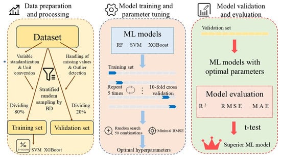
Figure 1. Flowchart of the development of ML models. ML, machine learning; RF, random forest; SVM, support vector machine; XGBoost, extreme gradient boosting; R², coefficient of determination; RMSE, root mean squared error; MAE, mean absolute error.

2.4. Model Development and Performance Metrics

The performance of each predictive model was rigorously assessed using three standard regression metrics: the coefficient of determination (R²), the root mean square error and the mean absolute error (MAE). These metrics quantify model fit and error magnitude, and were calculated based on the observed and predicted BD values using the following definitions:

$$R^2=1-{\displaystyle \frac{\sum _{i=1}^n{(y_{obs}-y_{pred})}^2}{\sum _{i=1}^n{(y_{obs}-{\overline{y}}_{obs})}^2}}$$

(4)

$$RMSE=\sqrt{{\displaystyle \frac{1}{n}}\sum _{i=1}^n{(y_{obs}-y_{pred})}^2}$$

(5)

$$MAE={\displaystyle \frac{1}{n}}\sum _{i=1}^n\left|y_{obs}-y_{pred}\right|$$

(6)

where ${\mathrm{y}}_{\mathrm{o}\mathrm{b}\mathrm{s}}$ is the observed BD value, ${\mathrm{y}}_{\mathrm{p}\mathrm{r}\mathrm{e}\mathrm{d}}$ is the predicted BD value from the models, ${\overline{\mathrm{y}}}_{\mathrm{o}\mathrm{b}\mathrm{s}}$ is the mean of the observed BD value, and n is the amount of data points in each model set.

All ML models were developed within the RStudio (v 4.3.1) statistical computing environment [56]. The specific R packages (Version 1.7-16) utilized for model implementation were: e1071 [57] for the Support Vector Machine, xgboost [58] for the Extreme Gradient Boosting, and randomForest [55] for the Random Forest model.

3. Results

3.1. Variation in Soil Physical Properties with Depth

The variation in soil bulk density with depth across the three distinct study sites is illustrated in Figure 2. Overall, a consistent trend of increasing BD with depth was observed across all locations, supporting findings from multiple European datasets [2]. Specifically, the BD in the 10–20 cm layer was generally higher than that recorded in the 0–10 cm surface layer, indicating subsurface compaction.

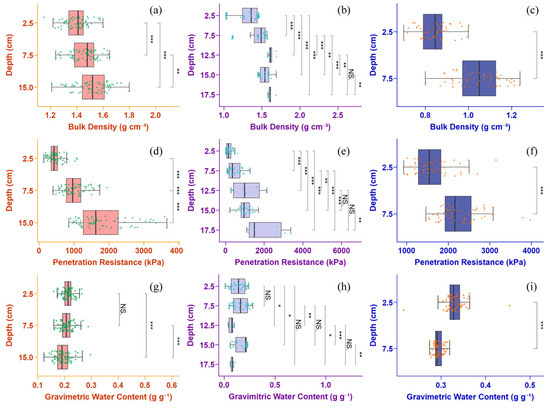
Figure 2. Variation in soil bulk density with depth at Site 1 (a), Site 2 (b) and Site 3 (c); and penetration resistance with depth at Site 1 (d), Site 2 (e) and Site 3 (f); and gravimetric water content with depth at Site 1 (g), Site 2 (h) and Site 3 (i). ‘***’, ‘**’, ‘*’, and ‘NS.’ indicate significant differences at p < 0.001, p < 0.01, p < 0.05 and not significant, respectively.

At Site 1, the mean BD value in the 0–10 cm layer was 1.43 g cm⁻³, while the 10–20 cm layer had an average of 1.52 g cm⁻³. At Site 2, the BD averaged 1.36 g cm⁻³ in the 0–10 cm layer and 1.56 g cm⁻³ in the 10–20 cm layer, exhibiting slightly higher compaction in the subsurface. At Site 3, the average BD was lower, with 0.84 g cm⁻³ in the 0–5 cm layer and 1.04 g cm⁻³ in the 5–10 cm layer, reflecting the high organic matter and clayey texture characteristic of rainforest soils. In the upper 0–10 cm layer, the highest soil BD recorded was 1.46 g cm⁻³ (at a depth of 7.5 cm), while the lowest recorded value, 1.04 g cm⁻³, was observed at Site 3. The compaction levels in the 10–20 cm layer at Site 1 and Site 2 were notably similar, with both exceeding 1.50 g cm⁻³.

Figure 2 also effectively visualizes the corresponding variation in PR with depth across the three study sites, revealing a highly synchronous trend with the BD data. In general, PR consistently increased with depth, mirroring the compaction patterns: At Site 1, the average PR was 743 kPa in the 0–10 cm layer, more than doubling to 1833 kPa in the 10–20 cm layer. Site 2 showed lower resistance in the surface layer (325 kPa) and a subsurface average of 1248 kPa (10–20 cm). Site 3 reflected its highly structured nature and recorded notably high PR values, averaging 1622 kPa (0–5 cm) and peaking at 2275 kPa in the 5–10 cm layer. In the shallow 0–10 cm layer, the highest PR value (1622 kPa) was observed at Site 3 (at 2.5 cm depth), significantly exceeding the 1069 kPa recorded at the much deeper 15 cm layer at Site 2. The absolute peak PR value for the entire dataset (2275 kPa) was recorded at Site 3 at a depth of 7.5 cm. In the deeper 10–20 cm layer, the PR at Site 1 (1833 kPa) remained higher than that observed at Site 2 (1248 kPa).

The soil samples exhibited distinct variability in GW, which is attributable to the diverse climatic and environmental conditions of the study sites. A general trend of GW decreasing with increasing soil depth was observed across the dataset. In the 0–10 cm surface layer, the average GW was highest at Site 3 (0.312 g g⁻¹), reflecting its tropical rainforest climate. This was followed by Site 1 (0.211 g g⁻¹) and Site 2 (0.148 g g⁻¹). In the deeper 10–20 cm layer, the average GW was 0.194 g g⁻¹ at Site 1 and 0.106 g g⁻¹ at Site 2. The GW at Site 1 demonstrated remarkable uniformity between the 0–10 cm and 10–20 cm layers, suggesting a more even distribution of moisture throughout the surface soil profile. Conversely, Site 2 recorded the lowest overall moisture content, with the 10–20 cm layer being significantly drier than the 0–10 cm layer. This pronounced disparity suggests potentially restrictive water infiltration into the deeper soil horizons at this location.

The general trend across all three study sites was a consistent increase in BD and PR with soil depth, while GW exhibited a corresponding decrease (Figure 2). However, an observed anomaly occurred in the 10–20 cm layer at Site 2: BD and PR values initially decreased before increasing with depth, while the trend for GW was inversed, initially increasing and then decreasing. This anomaly merits further mechanistic analysis. Furthermore, the inverse relationship between soil moisture and the mechanical properties (PR and BD) was uniformly observed across the dataset, consistent with findings in previous research [33,38].

3.2. Performance of Models in the Training Stage

Two traditional empirical models (MLR and MNLR) and three ML models (RF, SVM, and XGB) were rigorously applied to predict soil BD using PR and GW. The comparative performance of all five models during the training phase is clearly illustrated in Figure 3.

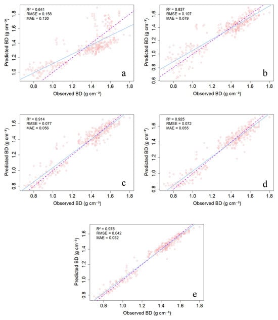
Figure 3. Performance of two baseline models: (a) MLR, (b) MNLR, and three ML algorithms: (c) SVM, (d) XGB, and (e) RF on training dataset. The purple dashed line represents the 1:1 line, while the blue solid line represents the fitted line.

The MLR model exhibited the poorest performance, achieving a R² of only 0.641. The MNLR model showed a moderate improvement in predictive accuracy, with an R² of 0.837.

In stark contrast, all ML models—RF, SVM, and XGB—achieved significantly superior performance over the traditional models. Compared to MLR, the R² values increased by 52.1% (RF), 44.3% (XGB), and 42.6% (SVM); the RF model exhibited the highest predictive capacity with an R² of 0.975. Compared to the nonlinear baseline MNLR, the ML models still demonstrated noticeable improvements in R² by 16.5% (RF), 10.5% (XGB), and 8.42% (SVM).

This comparative analysis definitively established the superior ability of ML algorithms to capture the complex, nonlinear relationship between BD, PR, and GW compared to traditional empirical models.

3.3. Performance of Models in the Validation Stage

During the crucial independent validation phase, all three ML models (RF, SVM, and XGB) conclusively demonstrated superior and robust performance compared to the traditional empirical models (MLR and MNLR) (Figure 4). Consistent with the training results, the RF model was identified as a more superior algorithm for BD prediction on the unseen data, with R² value of 0.932, RMSE value of 0.074 g cm⁻³, and MAE value of 0.058 g cm⁻³. The predictive capacity of the XGB model was slightly lower than that of RF and SVM, but the overall performance across all three ML models was exceptionally high, with R² values consistently exceeding 0.89. This high and stable performance across the independent validation set unequivocally confirms the strong generalization ability of the ML algorithms in capturing the complex, nonlinear relationships among BD, PR, and GW. The similarity in results between the training and validation phases indicates that the models, particularly RF, successfully learned the underlying physical relationships without suffering from overfitting, making them reliable tools for practical application.

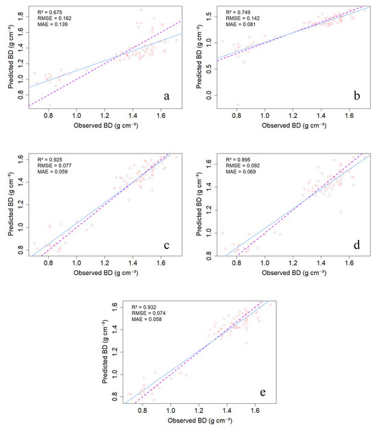
Figure 4. Performance of two baseline models: (a) MLR, (b) MNLR, and three ML algorithms: (c) SVM, (d) XGB, and (e) RF on validation dataset. The purple dashed line represents the 1:1 line, while the blue solid line represents the fitted line.

3.4. Comparative Evaluation of the Performance of Models

A critical aspect of model validation is the rigorous assessment of overfitting, a phenomenon that occurs when a function becomes too closely aligned with the training data, thereby compromising its generalization ability. The potential for overfitting is rigorously evaluated by calculating the difference (ΔR²) between the R² of the training set and the R² of the independent validation set; a smaller ΔR² value indicates superior model stability and generalization capacity [59,60,61].

The calculated ΔR² values were 0.043 for RF, 0.030 for XGB, and 0.011 for SVM. Evidently, the SVM model, exhibiting the smallest ΔR² of 0.011, definitively demonstrated the greatest stability among the three ML algorithms. This finding aligns with established literature which suggests that kernel-based models like SVM are often more robust and stable than tree-based ensemble methods such as XGB and RF [62], confirming that the SVM model is the least susceptible to overfitting in this predictive task.

Although intrinsic stability differences exist, all three ML models demonstrated excellent stability and strong generalization capacity. The R² values only decreased marginally between the training and validation sets—4.41% for RF and 3.24% for XGB—while the SVM model actually showed a slight increase of 1.30%. Crucially, the prediction accuracy error for all three ML models remained within 5% between the two phases, strongly suggesting that overfitting is not a practical concern. This conclusion is further supported by Figure 5, where the fitted regression lines for the training and validation sets lie in close proximity to each other and the ideal 1:1 line. This evidence collectively indicates that the models are highly stable, possess excellent predictive accuracy, and exhibit high potential for the robust prediction of soil BD using PR and GW.

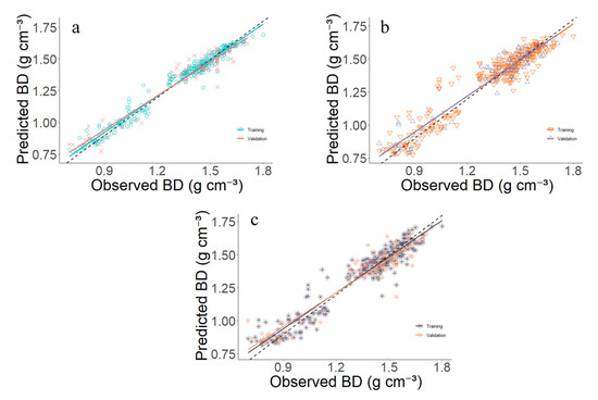
Figure 5. Comparative stability analysis of (a) RF, (b) SVM, and (c) XGB. The black dashed line represents the 1:1 line and solid lines of different colors represent the fitted lines for the corresponding datasets.

All three ML models underwent 10 × 5 repeated cross-validation. The 50 independent resampled results obtained were subjected to t-tests, yielding the outcomes presented in Table 3. The t-value of 3.538024 indicates that RF and XGB exhibit the greatest disparity, with this difference being highly significant (p < 0.01). As shown in Figure 6, the difference between SVM and XGB is significant (p < 0.05), while the difference between RF and SVM is not significant (p > 0.05). The 50 independent resampling results similarly indicate that RF has the highest R² value, followed by SVM, with XGB having the lowest.

Table 3. Paired t-test analysis of ML models performance using 10 × 5 repeated cross-validation. Effect size benchmarks: small (0.2), medium (0.5), large (0.8).

Model Comparison	t-Statistic	Degrees of Freedom	p-Value	Effect Size
RF vs. XGB	3.538024	49	0.00089	0.50035
SVM vs. XGB	2.112829	49	0.03973	0.29879
RF vs. SVM	1.145433	49	0.25759	NA

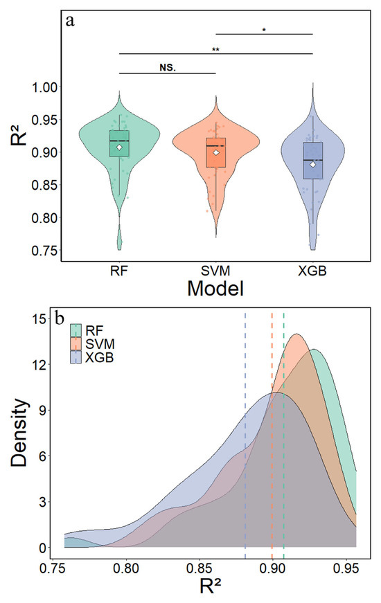
Figure 6. Distribution characteristics of R² values of ML models from repeated cross-validation. (a) Violin plots with significance annotations showing the distribution of R² values for three models, where ‘*’ indicates p < 0.05, ‘**’ indicates p < 0.01, and ‘NS.’ indicates not significant, respectively. (b) Density distribution plots displaying the probability density of R² values for each model, with dashed lines indicating mean values.

In both phases, the R² for all ML models consistently exceeded 0.89, demonstrating a high and stable level of predictive accuracy. Furthermore, the ML models achieved substantially lower RMSE and MAE values than MLR and MNLR. This stable and accurate performance on both known and independent data establishes that the ML algorithms not only effectively captured the complex relationships within the training set but also possessed robust generalization capabilities, making them highly reliable for predicting soil BD under diverse and unknown field conditions.

4. Discussion

4.1. Mechanistic Interpretation of Site-Specific Trends in Relation to Model Inputs

Our site-specific data, which served as the foundation for the ML models, revealed distinct patterns that can be mechanistically explained by local conditions and management practices, thereby validating the physical relevance of the predictor variables (PR and GW).

At Site 2, the anomaly observed in the 10–20 cm layer—where BD and PR initially decreased before increasing with depth—is a direct manifestation of long-term shallow rotary tillage [51]. This practice, with a working depth of only 10–12 cm, has led to the formation of a compacted plow pan just below the tilled layer. Our data clearly captures this phenomenon: the sharp increase in BD and PR beginning at approximately 12.5 cm (Figure 2b,e). This finding underscores why PR measurements, which are highly sensitive to such subsurface mechanical barriers, are a powerful predictor for BD in managed agricultural systems. The corresponding GW data at this site showed the lowest values in the dataset (Figure 2h), further exacerbating the high PR and BD in the subsoil due to reduced lubricating effects and increased soil strength.

Conversely, the low BD values at Site 3 align with its tropical rainforest ecology. Despite historical logging impacts [52,63], the high annual rainfall and the soil’s clayey, well-aggregated structure (typical of Oxisols) appear to confer resilience against persistent compaction. This is reflected in our dataset as a cluster of low BD values associated with high GW (Figure 2c,i). However, the exceptionally high PR values at this site, particularly in the 5–10 cm layer (peaking at 2275 kPa), seem counterintuitive given the low BD. This can be explained by prolonged waterlogging, which can lead to soil particle reorganization and age-hardening phenomena [64,65], increasing strength without a corresponding increase in density. This complex interplay, successfully captured by our ML models, highlights that the PR-GW-BD relationship is non-unique and context-dependent, necessitating sophisticated algorithms like RF and SVM to decode it.

4.2. Dominant Influence of Soil Moisture and Identification of a Critical Threshold

Our results move beyond establishing the feasibility of prediction and provide deep insights into the relative importance of the predictors and the nature of their relationship with BD. The SHAP analysis derived from our models conclusively identified GW as the dominant predictor of soil BD, significantly outweighing the influence of PR (Figure 7).

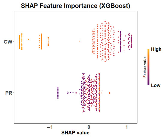
Figure 7. The SHAP value computed by the XGB model indicates the importance of predictive factors.

This finding is a direct quantification of a fundamental soil physical principle: soil mechanical stability is profoundly sensitive to moisture content [66]. The strong negative SHAP value for GW indicates that, within the context of our integrated dataset, a decrease in soil moisture was the primary driver of an increase in BD. Soil moisture content is widely regarded as the most critical single variable governing soil compaction [46,67], as changes in moisture level directly alter the soil’s pre-consolidation pressure, thereby significantly affecting its bulk physical properties [68]. Our ML models have not just captured this relationship but have quantified its paramount importance relative to PR.

A more nuanced finding from our analysis is the nonlinear and threshold-dependent relationship between BD and PR, which is critically mediated by GW. The visualization of this relationship across different GW intervals (Figure 8) reveals a critical transition point at approximately GW = 0.15 g g⁻¹.

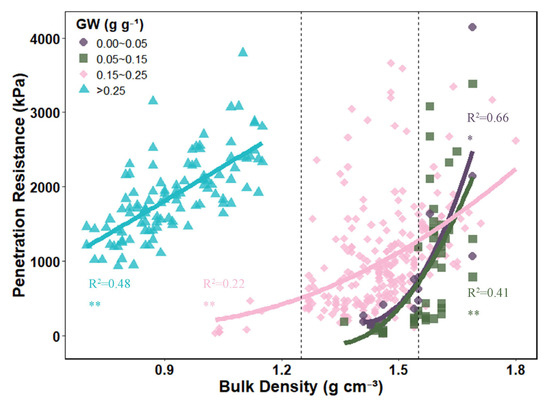
Figure 8. Synchronized changes between soil bulk density and penetration resistance at different gravimetric water content intervals. The solid lines represent the fitted lines. The dashed lines represent BD = 1.25 g cm⁻³ and 1.55 g cm⁻³, respectively. ‘**’ and ‘*’ indicate significant differences at p < 0.01 and p < 0.05, respectively.

Above this threshold (GW > 0.15 g g⁻¹), the trend line between BD and PR is relatively flat. This regime is typically associated with higher moisture (GW > 0.25 g g⁻¹) and lower density (BD < 1.25 g cm⁻³) conditions, where sufficient soil moisture maintains particle lubrication and plasticity. Consequently, changes in BD do not provoke a strong, immediate response in PR, and soils are less susceptible to drastic strength changes from compaction.

Below this threshold (GW < 0.15 g g⁻¹), the relationship steepens dramatically. In this dry, high-density state (where BD frequently exceeds 1.55 g cm⁻³), the lubricating effect of water diminishes, and soil strength becomes increasingly dependent on cohesion and internal friction [27,69]. Here, even a small increase in BD leads to a disproportionately large increase in PR, marking a state of high mechanical sensitivity and compaction risk.

Beyond the immediate effect of water presence, GW significantly influences soil structure through the wetting and drying cycle. As soil dries, microstructural rearrangements occur, leading to decreased soil compressibility and tighter textures due to volume shrinkage. This process of rearrangement and particle bonding forms new structural systems, consequently impacting aggregate formation, water retention capacity, and overall structural stability [70,71]. Furthermore, reduced moisture content increases the particle conductivity coefficient per unit volume [31,72,73]. As moisture drops, the lubricating effect of water diminishes, and soil strength becomes increasingly dependent on cohesion and internal friction between particles [27,69]. In this dry state, even a small increase in BD leads to a disproportionately large increase in PR. This zone represents a state of high mechanical sensitivity and compaction risk.

This heightened sensitivity at low moisture levels is attributed to several physical factors [33,74,75]. Firstly, as PR heavily relies on soil cohesion and bulk density, compression around and below the penetrometer probe becomes more significant. Secondly, the friction component between the soil and the penetrometer metal becomes more pronounced, given the reduction in the water’s lubricating effect. Finally, the increase in the angle of internal friction with decreasing moisture inherently indicates higher soil strength at lower moisture levels. Although PR is relatively high at lower moisture levels (as discussed in Section 3.1)—a phenomenon often related to local climate, soil texture, and wet-dry cycling processes—it reinforces the conclusion that PR should not be used directly as a sole measure of soil compaction. The necessity of incorporating GW to define this 0.15 g g⁻¹ critical threshold is essential for accurately predicting BD.

4.3. Comparative Advantages of Machine Learning over Traditional Regression Models

The rigorous evaluation of traditional empirical models and advanced ML models in this study yielded clear evidence regarding their predictive capabilities. The ML models—RF, SVM, and XGB—demonstrated significantly more accurate predictive capabilities, with accuracy improvements reaching more than 50% over the baseline MLR model. Furthermore, the minimal differences in performance among the three ML models (all exhibiting R² values exceeding 0.89) highlight their excellent and consistent potential for accurately predicting soil BD using PR and GW.

Traditional empirical methods are generally constrained by their inherent assumptions, which results in lower prediction accuracy when dealing with complex, real-world relationships. While MLR models offer advantages in interpretation and possess low computational costs, their fundamental limitation lies in their inability to capture nonlinear data structures, inevitably leading to high bias in the output results [76,77]. Although MNLR attempts to establish nonlinear relationships by incorporating squared and interaction terms, the accurate specification of the underlying functional form often requires extensive prior knowledge and empirical fitting, making it intrinsically challenging to accurately identify the full complexity of variable relationships.

The superior performance of MNLR compared to MLR in this study strongly indicated the presence of a pronounced nonlinear relationship among the input variables. For smaller datasets, simple traditional empirical models may suffice; however, the results conclusively support the premise that when dealing with significant nonlinearity and larger, diverse datasets, ML algorithms demonstrably outperform traditional empirical methods [46].

Compared to traditional empirical models, machine learning offers numerous advantages, fundamentally improving the accuracy of soil BD predictions. ML is an inherently flexible, data-driven approach rather than a rigid, assumption-bound one [78]. It excels at addressing complex curved regression problems, effectively handling anomalous input values, mitigating multicollinearity issues, and managing missing information [18,44]. The performance analysis in this study strongly supports this, with ML models achieving significant improvements over their empirical counterparts. While our results confirm the superior predictive accuracy of ML models within the domain of our calibration data, we acknowledge the valuable role of traditional models like MNLR. Their simpler structure, interpretability, and potentially greater robustness for extrapolation or use in data-sparse environments remain significant advantages. The choice between model types should be guided by the specific application context, weighing the need for highest possible accuracy against requirements for transparency, transferability, and operational simplicity. It should be noted that while the ML models demonstrated superior predictive performance within the scope of this study, their application to significantly different environmental conditions or regions with limited calibration data requires careful validation. Traditional linear models may offer advantages in such scenarios due to their greater transparency and transferability.

Among the specific algorithms utilized, SVM leverage kernel functions to transform low-dimensional inputs into high-dimensional space, thereby generating optimal decision hyperplanes for regression tasks [79,80]. The mechanism by which the distance between the support vectors and these hyperplanes is optimized results in low generalization error and computational stability, which is why SVM is typically less susceptible to overfitting [76,81,82]. Conversely, while XGB, based on tree regression, offers faster training speed, its numerous hyperparameters require extensive experience and experimentation for optimal tuning [54,58]. Although studies like [24] have shown XGB to be the best predictor among some ML models, this research revealed that all three ML models attained high predictive accuracy, yet the tree-based models (RF and XGB) proved less stable than SVM (as confirmed by the minimal ΔR² value). Therefore, due to its superior stability and minimal generalization error, the SVM model is recommended for practical soil BD prediction using PR and GW data.

The successful implementation of machine learning inherently relies on prior knowledge for the judicious selection of input parameters [83]. In this study, the choice of BD and PR was founded on their established role as common physical properties used to quantify soil compaction [84], supported by the close physical and non-linear relationships that exist between BD and PR [38,51,85]. Furthermore, the inclusion of GW was essential, as its significant impact on soil compaction is well-documented [38,46,67]. This informed selection strategy enabled the ML models to effectively capture the underlying and complex physical relationships between the input and output variables, leading to high predictive accuracy.

However, the architecture of the model can also influence the utility of predictions. Although ML algorithms are exceptionally successful in establishing highly accurate mathematical relationships, their inherent “black box” nature—the difficulty in fully interpreting the process by which a prediction is generated—remains a limitation to their widespread application and acceptance in fields relying on physical mechanisms [83].

Nevertheless, by coupling the high accuracy of the models with the SHAP value analysis in this study, the contribution of each predictor was quantified and mechanistically justified, thereby offering a crucial step toward demystifying the model’s output and increasing its utility for applied soil science.

4.4. Limitations and Perspectives

The integration of heterogeneous data from multiple sites undoubtedly influences the predictive performance of the unified model. While this aggregation enhances the model’s robustness and generalizability across diverse soil conditions, it may inherently smooth over some site-specific relationships, potentially at the cost of optimal precision for any single location. This trade-off between universality and locality represents a fundamental consideration in pedotransfer function development. Our analysis indeed suggests that developing site-specific models could yield higher prediction accuracy for individual sites, as such models would be finely calibrated to local soil characteristics and management practices. However, this approach necessitates sufficient calibration data for each specific environment, which is often a practical limitation. Therefore, the choice between a unified global model and localized models should be guided by the application context, weighing the need for broad applicability against the requirement for maximum precision at a given location. Future research could productively explore hybrid or meta-learning modeling frameworks that strategically leverage the strengths of both aggregated and site-specific approaches.

The model developed in this study, while robust, was established under specific constraints, primarily focusing on surface soils (0–20 cm) and involving a limited range of soil types and textures. This specialization means that the model’s direct applicability is constrained: should there be significant changes in the soil depth of interest or the measurement instruments used, the model would likely require recalibration or parameter adjustment for effective retraining. Moreover, the timing of field sampling represents a critical factor, as short-term variations in agricultural management practices and precipitation can significantly increase data uncertainty, a common challenge in soil physics modeling.

Therefore, future research should strategically aim to enhance the model’s generalizability and predictive accuracy by broadening its scope. This includes incorporating additional soil properties such as soil porosity, pore size distribution, a wider range of soil texture types, and organic matter content, as these factors have been shown to significantly influence BD [86,87,88,89]. Furthermore, expanding the range of soil depths and types, along with integrating more comprehensive environmental variables, will naturally enhance the model’s overall applicability across different regions. Finally, exploration of different ML models and sophisticated ensemble methods is recommended to identify potential avenues for incrementally improving prediction accuracy and model efficiency.

5. Conclusions

This study successfully validated the immense potential of predicting soil BD using PR and GW combined with ML models by integrating multi-site field sampling and published data. The three ML models (RF, SVM, and XGB) achieved significantly higher prediction accuracy compared to traditional empirical models, with R² values all exceeding 0.89 on the validation set. Specifically, the RF model achieved the highest predictive accuracy (R² = 0.932), while the SVM model demonstrated superior model stability (difference between training and validation R², ΔR² = 0.011). Considering the critical need for robustness and generalization ability in practical field applications, the SVM model is therefore recommended for reliable, widespread BD prediction. Furthermore, the analysis confirmed that GW was the most critical factor for estimating BD, underscoring the dominant role of soil moisture in determining compaction, and establishing a critical threshold of GW = 0.15 g g⁻¹ in the nonlinear relationship between BD and PR for our study conditions, below which property changes are significantly accelerated, while noting this value may vary with soil properties. This novel approach, leveraging readily available field measurements (PR and GW) with ML techniques, offers a feasible, high-precision, non-destructive, and low-cost alternative for acquiring soil BD data, though future work should expand the dataset’s diversity to enhance model universality.

References

- Al-Shammary, A.A.G.; Kouzani, A.Z.; Kaynak, A.; Khoo, S.Y.; Norton, M.; Gates, W. Soil Bulk Density Estimation Methods: A Review. Pedosphere 2018, 28, 581–596. [Google Scholar] [CrossRef]
- Panagos, P.; De Rosa, D.; Liakos, L.; Labouyrie, M.; Borrelli, P.; Ballabio, C. Soil Bulk Density Assessment in Europe. Agric. Ecosyst. Environ. 2024, 364, 108907. [Google Scholar] [CrossRef]
- Al-Shammary, A.A.G.; Kouzani, A.; Kaynak, A.; Khoo, S.Y.; Norton, M. Experimental Investigation of Thermo-Physical Properties of Soil Using Solarisation Technology. Am. J. Appl. Sci. 2017, 14, 649–661. [Google Scholar] [CrossRef][Green Version]
- Evett, S.R.; Agam, N.; Kustas, W.P.; Colaizzi, P.D.; Schwartz, R.C. Soil Profile Method for Soil Thermal Diffusivity, Conductivity and Heat Flux: Comparison to Soil Heat Flux Plates. Adv. Water Resour. 2012, 50, 41–54. [Google Scholar] [CrossRef]
- Xu, L.; He, N.; Yu, G. Methods of Evaluating Soil Bulk Density: Impact on Estimating Large Scale Soil Organic Carbon Storage. CATENA 2016, 144, 94–101. [Google Scholar] [CrossRef]
- Zheng, G.; Jiao, C.; Xie, X.; Cui, X.; Shang, G.; Zhao, C.; Zeng, R. Pedotransfer Functions for Predicting Bulk Density of Coastal Soils in East China. Pedosphere 2023, 33, 849–856. [Google Scholar] [CrossRef]
- Reichert, J.M.; Suzuki, L.E.A.S.; Reinert, D.J.; Horn, R.; Håkansson, I. Reference Bulk Density and Critical Degree-of-Compactness for No-till Crop Production in Subtropical Highly Weathered Soils. Soil Tillage Res. 2009, 102, 242–254. [Google Scholar] [CrossRef]
- Shi, L.; O’Rourke, S.; De Santana, F.B.; Daly, K. Prediction of Soil Bulk Density in Agricultural Soils Using Mid-Infrared Spectroscopy. Geoderma 2023, 434, 116487. [Google Scholar] [CrossRef]
- Pires, L.F.; Rosa, J.A.; Pereira, A.B.; Arthur, R.C.J.; Bacchi, O.O.S. Gamma-Ray Attenuation Method as an Efficient Tool to Investigate Soil Bulk Density Spatial Variability. Ann. Nucl. Energy 2009, 36, 1734–1739. [Google Scholar] [CrossRef]
- Zhou, J.; Li, E.; Wei, H.; Li, C.; Qiao, Q.; Armaghani, D.J. Random Forests and Cubist Algorithms for Predicting Shear Strengths of Rockfill Materials. Appl. Sci. 2019, 9, 1621. [Google Scholar] [CrossRef]
- Zeng, C.; Wang, Q.; Zhang, F.; Zhang, J. Temporal Changes in Soil Hydraulic Conductivity with Different Soil Types and Irrigation Methods. Geoderma 2013, 193–194, 290–299. [Google Scholar] [CrossRef]
- Casanova, M.; Tapia, E.; Seguel, O.; Salazar, O. Direct Measurement and Prediction of Bulk Density on Alluvial Soils of Central Chile. Chil. J. Agric. Res. 2016, 76, 105–113. [Google Scholar] [CrossRef]
- Martín, M.Á.; Reyes, M.; Taguas, F.J. Estimating Soil Bulk Density with Information Metrics of Soil Texture. Geoderma 2017, 287, 66–70. [Google Scholar] [CrossRef]
- Nanko, K.; Ugawa, S.; Hashimoto, S.; Imaya, A.; Kobayashi, M.; Sakai, H.; Ishizuka, S.; Miura, S.; Tanaka, N.; Takahashi, M.; et al. A Pedotransfer Function for Estimating Bulk Density of Forest Soil in Japan Affected by Volcanic Ash. Geoderma 2014, 213, 36–45. [Google Scholar] [CrossRef]
- Akpa, S.I.C.; Ugbaje, S.U.; Bishop, T.F.A.; Odeh, I.O.A. Enhancing Pedotransfer Functions with Environmental Data for Estimating Bulk Density and Effective Cation Exchange Capacity in a Data-sparse Situation. Soil Use Manag. 2016, 32, 644–658. [Google Scholar] [CrossRef]
- Yi, X.; Li, G.; Yin, Y. Pedotransfer Functions for Estimating Soil Bulk Density: A Case Study in the Three-River Headwater Region of Qinghai Province, China. Pedosphere 2016, 26, 362–373. [Google Scholar] [CrossRef]
- Choudhury, B.U.; Santra, P.; Singh, N.; Chakraborty, P. Development of Land-Use-Specific Pedotransfer Functions for Predicting Bulk Density of Acidic Topsoil in Eastern Himalayas (India). Geoderma Reg. 2023, 34, e00671. [Google Scholar] [CrossRef]
- Chen, Z.; Xue, J.; Wang, Z.; Zhou, Y.; Deng, X.; Liu, F.; Song, X.; Zhang, G.; Su, Y.; Zhu, P.; et al. Ensemble Modelling-Based Pedotransfer Functions for Predicting Soil Bulk Density in China. Geoderma 2024, 448, 116969. [Google Scholar] [CrossRef]
- Chen, S.; Chen, Z.; Zhang, X.; Luo, Z.; Schillaci, C.; Arrouays, D.; Richer-de-Forges, A.C.; Shi, Z. European Topsoil Bulk Density and Organic Carbon Stock Database (0–20 cm) Using Machine-Learning-Based Pedotransfer Functions. Earth Syst. Sci. Data 2024, 16, 2367–2383. [Google Scholar] [CrossRef]
- Bauer, T.; Strauss, P.; Murer, E. A Photogrammetric Method for Calculating Soil Bulk Density. J. Plant Nutr. Soil Sci. 2014, 177, 496–499. [Google Scholar] [CrossRef]
- Beamish, D. Relationships between Gamma-Ray Attenuation and Soils in SW England. Geoderma 2015, 259–260, 174–186. [Google Scholar] [CrossRef]
- Lobsey, C.R.; Viscarra Rossel, R.A. Sensing of Soil Bulk Density for More Accurate Carbon Accounting. Eur. J. Soil Sci. 2016, 67, 504–513. [Google Scholar] [CrossRef]
- Fu, Y.; Lu, Y.; Heitman, J.; Ren, T. Root Influences on Soil Bulk Density Measurements with Thermo-Time Domain Reflectometry. Geoderma 2021, 403, 115195. [Google Scholar] [CrossRef]
- Wan, H.; Qi, H.; Shang, S. Estimating Soil Water and Salt Contents from Field Measurements with Time Domain Reflectometry Using Machine Learning Algorithms. Agric. Water Manag. 2023, 285, 108364. [Google Scholar] [CrossRef]
- Gates, Z.W.; Galagedara, L.W.; Ziegler, S.E. Combining Ground Penetrating Radar Methodologies Enables Large-scale Mapping of Soil Horizon Thickness and Bulk Density in Boreal Forests. Soil Use Manag. 2023, 39, 1289–1303. [Google Scholar] [CrossRef]
- Colombi, T.; Torres, L.C.; Walter, A.; Keller, T. Feedbacks between Soil Penetration Resistance, Root Architecture and Water Uptake Limit Water Accessibility and Crop Growth—A Vicious Circle. Sci. Total Environ. 2018, 626, 1026–1035. [Google Scholar] [CrossRef]
- Tian, M.; Qin, S.; Whalley, W.R.; Zhou, H.; Ren, T.; Gao, W. Changes of Soil Structure under Different Tillage Management Assessed by Bulk Density, Penetrometer Resistance, Water Retention Curve, Least Limiting Water Range and X-Ray Computed Tomography. Soil Tillage Res. 2022, 221, 105420. [Google Scholar] [CrossRef]
- Yao, S.; Teng, X.; Zhang, B. Effects of Rice Straw Incorporation and Tillage Depth on Soil Puddlability and Mechanical Properties during Rice Growth Period. Soil Tillage Res. 2015, 146, 125–132. [Google Scholar] [CrossRef]
- Jiang, Q.; Cao, M.; Wang, Y.; Wang, J. Estimating Soil Penetration Resistance of Paddy Soils in the Plastic State Using Physical Properties. Agronomy 2020, 10, 1914. [Google Scholar] [CrossRef]
- Blanco-Canqui, H. Does Biochar Application Alleviate Soil Compaction? Review and Data Synthesis. Geoderma 2021, 404, 115317. [Google Scholar] [CrossRef]
- Liu, B.; Fan, H.; Jiang, Y.; Ma, R. Evaluation of Soil Macro-Aggregate Characteristics in Response to Soil Macropore Characteristics Investigated by X-Ray Computed Tomography under Freeze-Thaw Effects. Soil Tillage Res. 2023, 225, 105559. [Google Scholar] [CrossRef]
- Suzuki, L.E.A.S.; Reinert, D.J.; Pillon, C.N.; Reichert, J.M. Mechanical Resistance to Penetration for Improved Diagnosis of Soil Compaction at Grazing and Forest Sites. Forests 2024, 15, 1369. [Google Scholar] [CrossRef]
- Vaz, C.M.P.; Manieri, J.M.; De Maria, I.C.; Tuller, M. Modeling and Correction of Soil Penetration Resistance for Varying Soil Water Content. Geoderma 2011, 166, 92–101. [Google Scholar] [CrossRef]
- Grzesiak, S.; Grzesiak, M.T.; Hura, T.; Marcińska, I.; Rzepka, A. Changes in Root System Structure, Leaf Water Potential and Gas Exchange of Maize and Triticale Seedlings Affected by Soil Compaction. Environ. Exp. Bot. 2013, 88, 2–10. [Google Scholar] [CrossRef]
- Çarman, K. Compaction Characteristics of Towed Wheels on Clay Loam in a Soil Bin. Soil Tillage Res. 2002, 65, 37–43. [Google Scholar] [CrossRef]
- Kormanek, M. Use of Impact Penetrometer to Determine Changes in Soil Compactness After Entracon Sioux EH30 Timber Harvesting. Croat. J. For. Eng. 2022, 43, 325–337. [Google Scholar] [CrossRef]
- Otto, R.; Silva, A.P.; Franco, H.C.J.; Oliveira, E.C.A.; Trivelin, P.C.O. High Soil Penetration Resistance Reduces Sugarcane Root System Development. Soil Tillage Res. 2011, 117, 201–210. [Google Scholar] [CrossRef]
- Moraes, M.T.D.; Olbermann, F.J.R.; Bonetti, J.D.A.; Pilegi, L.R.; Costa, M.V.R.; Pacheco, V.; Rogers, C.D.; Guimarães, R.M.L. The Impacts of Cover Crop Mixes on the Penetration Resistance Model of an Oxisol under No-Tillage. Soil Tillage Res. 2024, 242, 106138. [Google Scholar] [CrossRef]
- Martínez-Fernández, J.; González-Zamora, A.; Sánchez, N.; Gumuzzio, A.; Herrero-Jiménez, C.M. Satellite Soil Moisture for Agricultural Drought Monitoring: Assessment of the SMOS Derived Soil Water Deficit Index. Remote Sens. Environ. 2016, 177, 277–286. [Google Scholar] [CrossRef]
- Singh, G.; Panda, R.K.; Mohanty, B.P. Spatiotemporal Analysis of Soil Moisture and Optimal Sampling Design for Regional-Scale Soil Moisture Estimation in a Tropical Watershed of India. Water Resour. Res. 2019, 55, 2057–2078. [Google Scholar] [CrossRef]
- Zhao, T.; Shi, J.; Lv, L.; Xu, H.; Chen, D.; Cui, Q.; Jackson, T.J.; Yan, G.; Jia, L.; Chen, L.; et al. Soil Moisture Experiment in the Luan River Supporting New Satellite Mission Opportunities. Remote Sens. Environ. 2020, 240, 111680. [Google Scholar] [CrossRef]
- Mane, S.; Das, N.; Singh, G.; Cosh, M.; Dong, Y. Advancements in Dielectric Soil Moisture Sensor Calibration: A Comprehensive Review of Methods and Techniques. Comput. Electron. Agric. 2024, 218, 108686. [Google Scholar] [CrossRef]
- Yao, Y.; Fan, J.; Li, J. A Review of Advanced Soil Moisture Monitoring Techniques for Slope Stability Assessment. Water 2025, 17, 390. [Google Scholar] [CrossRef]
- Martin, M.P.; Seen, D.L.; Boulonne, L.; Jolivet, C.; Nair, K.M.; Bourgeon, G.; Arrouays, D. Optimizing Pedotransfer Functions for Estimating Soil Bulk Density Using Boosted Regression Trees. Soil Sci. Soc. Am. J. 2009, 73, 485–493. [Google Scholar] [CrossRef]
- Fernandes, M.M.H.; Coelho, A.P.; Silva, M.F.D.; Bertonha, R.S.; Queiroz, R.F.D.; Furlani, C.E.A.; Fernandes, C. Estimation of Soil Penetration Resistance with Standardized Moisture Using Modeling by Artificial Neural Networks. CATENA 2020, 189, 104505. [Google Scholar] [CrossRef]
- Bayat, H.; Asghari, S.; Rastgou, M.; Sheykhzadeh, G.R. Estimating Proctor Parameters in Agricultural Soils in the Ardabil Plain of Iran Using Support Vector Machines, Artificial Neural Networks and Regression Methods. CATENA 2020, 189, 104467. [Google Scholar] [CrossRef]
- Li, J.; Liu, F.; Shi, W.; Du, Z.; Deng, X.; Ma, Y.; Shi, X.; Zhang, M.; Li, Q. Including Soil Depth as a Predictor Variable Increases Prediction Accuracy of SOC Stocks. Soil Tillage Res. 2024, 238, 106007. [Google Scholar] [CrossRef]
- Dai, L.; Wang, Z.; Zhuo, Z.; Ma, Y.; Shi, Z.; Chen, S. Prediction of Soil Organic Carbon Fractions in Tropical Cropland Using a Regional Visible and Near-Infrared Spectral Library and Machine Learning. Soil Tillage Res. 2025, 245, 106297. [Google Scholar] [CrossRef]
- Guo, L.; Fan, G.; Zhang, Y.; Shen, Z. Estimating the Bulk Density in 0-20 cm of Tilled Soils in China’s Loess Plateau Using Support Vector Machine Modeling. Commun. Soil Sci. Plant Anal. 2019, 50, 1753–1763. [Google Scholar] [CrossRef]
- Fernandes, M.M.H.; Coelho, A.P.; Fernandes, C.; Silva, M.F.D.; Dela Marta, C.C. Estimation of Soil Organic Matter Content by Modeling with Artificial Neural Networks. Geoderma 2019, 350, 46–51. [Google Scholar] [CrossRef]
- Wang, H.; Wang, L.; Huang, X.; Gao, W.; Ren, T. An Empirical Model for Estimating Soil Penetrometer Resistance from Relative Bulk Density, Matric Potential, and Depth. Soil Tillage Res. 2021, 208, 104904. [Google Scholar] [CrossRef]
- DeArmond, D.; Ferraz, J.B.S.; Lovera, L.H.; Souza, C.A.S.D.; Corrêa, C.; Spanner, G.C.; Lima, A.J.N.; Dos Santos, J.; Higuchi, N. Impacts to Soil Properties Still Evident 27 Years after Abandonment in Amazonian Log Landings. For. Ecol. Manag. 2022, 510, 120105. [Google Scholar] [CrossRef]
- Huang, Y. Improved SVM-Based Soil-Moisture-Content Prediction Model for Tea Plantation. Plants 2023, 12, 2309. [Google Scholar] [CrossRef]
- Chen, T.; Guestrin, C. XGBoost: A Scalable Tree Boosting System. In Proceedings of the 22nd ACM SIGKDD International Conference on Knowledge Discovery and Data Mining, San Francisco, CA, USA, 13–17 August 2016; ACM: New York, NY, USA, 2016; pp. 785–794. [Google Scholar] [CrossRef]
- Breiman, L. Random Forests. Mach. Learn. 2001, 45, 5–32. [Google Scholar] [CrossRef]
- R Core Team. R: A Language and Environment for Statistical Computing. Vienna, Austria: R Foundation for Statistical Computing. 2023. Available online: https://www.r-project.org (accessed on 16 June 2023).
- Meyer, D.; Dimitriadou, E.; Hornik, K.; Weingessel, A.; Leisch, F. e1071: Misc Functions of the Department of Statistics, Probability Theory Group (Formerly: E1071). R Package Version 1.7-16. 2024. Available online: https://cran.r-project.org/package=e1071 (accessed on 16 September 2024).
- Chen, T.; He, T.; Benesty, M.; Khotilovich, V.; Tang, Y.; Cho, H.; Chen, K.; Mitchell, R.; Cano, I.; Zhou, T.; et al. xgboost: Extreme Gradient Boosting. R package version 1.7.11.1. 2025. Available online: https://CRAN.R-project.org/package=xgboost (accessed on 15 May 2025).
- Samani, S.; Vadiati, M.; Nejatijahromi, Z.; Etebari, B.; Kisi, O. Groundwater Level Response Identification by Hybrid Wavelet–Machine Learning Conjunction Models Using Meteorological Data. Environ. Sci. Pollut. Res. 2022, 30, 22863–22884. [Google Scholar] [CrossRef] [PubMed]
- Taşan, M.; Demir, Y.; Taşan, S.; Öztürk, E. Comparative Analysis of Different Machine Learning Algorithms for Predicting Trace Metal Concentrations in Soils under Intensive Paddy Cultivation. Comput. Electron. Agric. 2024, 219, 108772. [Google Scholar] [CrossRef]
- Wu, J.; Huang, C. Machine Learning-Supported Determination for Site-Specific Natural Background Values of Soil Heavy Metals. J. Hazard. Mater. 2025, 487, 137276. [Google Scholar] [CrossRef]
- Fan, J.; Yue, W.; Wu, L.; Zhang, F.; Cai, H.; Wang, X.; Lu, X.; Xiang, Y. Evaluation of SVM, ELM and Four Tree-Based Ensemble Models for Predicting Daily Reference Evapotranspiration Using Limited Meteorological Data in Different Climates of China. Agric. For. Meteorol. 2018, 263, 225–241. [Google Scholar] [CrossRef]
- DeArmond, D.; Emmert, F.; Lima, A.J.N.; Higuchi, N. Impacts of Soil Compaction Persist 30 Years after Logging Operations in the Amazon Basin. Soil Tillage Res. 2019, 189, 207–216. [Google Scholar] [CrossRef]
- McNabb, D.H.; Boersma, L. Evaluation of the Relationship between Compressibility and Shear Strength of Andisols. Soil Sci. Soc. Am. J. 1993, 57, 923–929. [Google Scholar] [CrossRef]
- Ampoorter, E.; Van Nevel, L.; De Vos, B.; Hermy, M.; Verheyen, K. Assessing the Effects of Initial Soil Characteristics, Machine Mass and Traffic Intensity on Forest Soil Compaction. For. Ecol. Manag. 2010, 260, 1664–1676. [Google Scholar] [CrossRef]
- Saffih-Hdadi, K.; Défossez, P.; Richard, G.; Cui, Y.-J.; Tang, A.-M.; Chaplain, V. A Method for Predicting Soil Susceptibility to the Compaction of Surface Layers as a Function of Water Content and Bulk Density. Soil Tillage Res. 2009, 105, 96–103. [Google Scholar] [CrossRef]
- Pöhlitz, J.; Rücknagel, J.; Schlüter, S.; Vogel, H.-J.; Christen, O. Computed Tomography as an Extension of Classical Methods in the Analysis of Soil Compaction, Exemplified on Samples from Two Tillage Treatments and at Two Moisture Tensions. Geoderma 2019, 346, 52–62. [Google Scholar] [CrossRef]
- Rücknagel, J.; Christen, O.; Hofmann, B.; Ulrich, S. A Simple Model to Estimate Change in Precompression Stress as a Function of Water Content on the Basis of Precompression Stress at Field Capacity. Geoderma 2012, 177–178, 1–7. [Google Scholar] [CrossRef]
- Souza, R.; Hartzell, S.; Freire Ferraz, A.P.; De Almeida, A.Q.; De Sousa Lima, J.R.; Dantas Antonino, A.C.; De Souza, E.S. Dynamics of Soil Penetration Resistance in Water-Controlled Environments. Soil Tillage Res. 2021, 205, 104768. [Google Scholar] [CrossRef]
- Pires, L.F.; Auler, A.C.; Roque, W.L.; Mooney, S.J. X-Ray Microtomography Analysis of Soil Pore Structure Dynamics under Wetting and Drying Cycles. Geoderma 2020, 362, 114103. [Google Scholar] [CrossRef] [PubMed]
- Pan, L.; Chen, Y.; Xu, Y.; Li, J.; Lu, H. A Model for Soil Moisture Content Prediction Based on the Change in Ultrasonic Velocity and Bulk Density of Tillage Soil under Alternating Drying and Wetting Conditions. Measurement 2022, 189, 110504. [Google Scholar] [CrossRef]
- Tang, C.-S.; Wang, D.-Y.; Shi, B.; Li, J. Effect of Wetting-Drying Cycles on Profile Mechanical Behavior of Soils with Different Initial Conditions. Catena 2016, 139, 105–116. [Google Scholar] [CrossRef]
- Zhang, B.; Jia, Y.; Fan, H.; Guo, C.; Fu, J.; Li, S.; Li, M.; Liu, B.; Ma, R. Soil Compaction Due to Agricultural Machinery Impact: A Systematic Review. Land Degrad. Dev. 2024, 35, 3256–3273. [Google Scholar] [CrossRef]
- Mulqueen, J.; Stafford, J.V.; Tanner, D.W. Evaluation of Penetrometers for Measuring Soil Strength. J. Terramech. 1977, 14, 137–151. [Google Scholar] [CrossRef]
- Moraes, M.T.D.; Debiasi, H.; Franchini, J.C.; Silva, V.R.D. Soil Penetration Resistance in a Rhodic Eutrudox Affected by Machinery Traffic and Soil Water Content. Eng. Agrícola 2013, 33, 748–757. [Google Scholar] [CrossRef]
- Abdallah, M.; Abu Talib, M.; Feroz, S.; Nasir, Q.; Abdalla, H.; Mahfood, B. Artificial Intelligence Applications in Solid Waste Management: A Systematic Research Review. Waste Manag. 2020, 109, 231–246. [Google Scholar] [CrossRef]
- Nguyen, X.C.; Nguyen, T.T.H.; La, D.D.; Kumar, G.; Rene, E.R.; Nguyen, D.D.; Chang, S.W.; Chung, W.J.; Nguyen, X.H.; Nguyen, V.K. Development of Machine Learning—Based Models to Forecast Solid Waste Generation in Residential Areas: A Case Study from Vietnam. Resour. Conserv. Recycl. 2021, 167, 105381. [Google Scholar] [CrossRef]
- Zhang, S.; Zhao, J.; Zhu, L. Predicting Removal Efficiency of Organic Pollutants by Soil Vapor Extraction Based on an Optimized Machine Learning Method. Sci. Total Environ. 2024, 927, 172438. [Google Scholar] [CrossRef]
- Balcan, M.-F.; Blum, A.; Vempala, S. Kernels as Features: On Kernels, Margins, and Low-Dimensional Mappings. Mach. Learn. 2006, 65, 79–94. [Google Scholar] [CrossRef]
- Teshome, F.T.; Bayabil, H.K.; Schaffer, B.; Ampatzidis, Y.; Hoogenboom, G.; Singh, A. Simulating Soil Hydrologic Dynamics Using Crop Growth and Machine Learning Models. Comput. Electron. Agric. 2024, 224, 109186. [Google Scholar] [CrossRef]
- Li, P.; Kwon, H.; Sun, L.; Lall, U.; Kao, J. A Modified Support Vector Machine Based Prediction Model on Streamflow at the Shihmen Reservoir, Taiwan. Int. J. Climatol. 2010, 30, 1256–1268. [Google Scholar] [CrossRef]
- Kumar, A.; Samadder, S.R.; Kumar, N.; Singh, C. Estimation of the Generation Rate of Different Types of Plastic Wastes and Possible Revenue Recovery from Informal Recycling. Waste Manag. 2018, 79, 781–790. [Google Scholar] [CrossRef]
- Wang, X.; Gao, Y.; Hou, J.; Yang, J.; Smits, K.; He, H. Machine Learning Facilitates Connections between Soil Thermal Conductivity, Soil Water Content, and Soil Matric Potential. J. Hydrol. 2024, 633, 130950. [Google Scholar] [CrossRef]
- Blanco-Canqui, H.; Ruis, S.J. No-Tillage and Soil Physical Environment. Geoderma 2018, 326, 164–200. [Google Scholar] [CrossRef]
- Vizioli, B.; Cavalieri-Polizeli, K.M.V.; Tormena, C.A.; Barth, G. Effects of Long-Term Tillage Systems on Soil Physical Quality and Crop Yield in a Brazilian Ferralsol. Soil Tillage Res. 2021, 209, 104935. [Google Scholar] [CrossRef]
- Gui, W.; You, Y.; Yang, F.; Zhang, M. Soil Bulk Density and Matric Potential Regulate Soil CO2 Emissions by Altering Pore Characteristics and Water Content. Land 2023, 12, 1646. [Google Scholar] [CrossRef]
- Du, Y.; Guo, S.; Wang, R.; Song, X.; Ju, X. Soil Pore Structure Mediates the Effects of Soil Oxygen on the Dynamics of Greenhouse Gases during Wetting–Drying Phases. Sci. Total Environ. 2023, 895, 165192. [Google Scholar] [CrossRef] [PubMed]
- Liu, X.; Rezaei Rashti, M.; Van Zwieten, L.; Esfandbod, M.; Rose, M.T.; Chen, C. Microbial Carbon Functional Responses to Compaction and Moisture Stresses in Two Contrasting Australian Soils. Soil Tillage Res. 2023, 234, 105825. [Google Scholar] [CrossRef]
- Thotakuri, G.; Chakraborty, P.; Singh, J.; Xu, S.; Kovács, P.; Iqbal, J.; Kumar, S. X-Ray Computed Tomography—Measured Pore Characteristics and Hydro-Physical Properties of Soil Profile as Influenced by Long-Term Tillage and Rotation Systems. CATENA 2024, 237, 107801. [Google Scholar] [CrossRef]
Disclaimer/Publisher’s Note: The statements, opinions and data contained in all publications are solely those of the individual author(s) and contributor(s) and not of MDPI and/or the editor(s). MDPI and/or the editor(s) disclaim responsibility for any injury to people or property resulting from any ideas, methods, instructions or products referred to in the content. |
© 2025 by the authors. Licensee MDPI, Basel, Switzerland. This article is an open access article distributed under the terms and conditions of the Creative Commons Attribution (CC BY) license (https://creativecommons.org/licenses/by/4.0/).