Lightweight Isotropic Convolutional Neural Network for Plant Disease Identification

Abstract

In today’s world, agricultural products are becoming increasingly scarce globally due to a variety of factors, and the early and accurate automatic identification of plant diseases can help ensure the stability and sustainability of agricultural production, improve the quality and safety of agricultural products, and help promote agricultural modernization and sustainable development. For this purpose, a lightweight deep isotropic convolutional neural network model, FoldNet, is designed for plant disease identification in this study. The model improves the architecture of residual neural networks by first folding the chain of the same blocks and then connecting these blocks with jump connections of different distances. Such a design allows the neural network to explore a larger receptive domain, enhancing its multiscale representation capability, increasing the direct propagation of information throughout the network, and improving the performance of the neural network. The FoldNet model achieved a recognition accuracy of 99.84% on the laboratory dataset PlantVillage using only 685k parameters and a recognition accuracy of 90.49% on the realistic scene dataset FGVC8 using only 516k parameters, which is competitive with other state-of-the-art models. In addition, as far as we know, our model is the first model that has fewer than 1M parameters while achieving state-of-the-art accuracy in plant disease identification. This proposal facilitates precision agriculture applications on mobile, low-end terminals.

1. Introduction

Plant diseases are one of the major causes of crop yield reduction and quality deterioration. With today’s dramatic population growth, the global population is expected to reach 9.7 billion by 2050, and there is an urgent need to find new ways to improve the yield and quality of agricultural products to meet the massive demand of a growing population [1]. As a new technology, precision agriculture, or smart farming, aims to improve agriculture’s efficiency and sustainability by using data and advanced technologies to make more informed, data-driven decisions about crop production and resource management [2]. By quickly and accurately identifying plant diseases, it can not only prevent the spread of plant diseases and protect the quality of plants, but also increase farmers’ income and reduce the cost of plant disease treatment. Early, rapid, and accurate disease identification and control can reduce the negative environmental impact, and using fewer chemicals and pesticides can reduce water and soil contamination. Consequently, it is necessary to study an efficient, accurate, and strongly robust automatic plant disease identification method, which is important to help farmers identify plant diseases and improve plant yield and quality.

In plant disease identification, image processing algorithms and traditional machine learning algorithms were commonly used in the early stages to identify plant diseases. After that, with the development of artificial intelligence, the application of deep learning algorithms in plant disease identification has achieved remarkable results, especially convolutional neural networks (CNN), which do not require pre-required processes such as segmentation and feature extraction and can automatically learn features in images as well as having excellent robustness and generalization ability [3]. More recently, inspired by the Transformer in Natural Language Processing (NLP) [4,5], Vision Transformer (ViT) [6] was the first attempt to use a transformer in the field of image recognition, and it achieved impressive results on the ImageNet dataset, demonstrating transformers’ potential in the image domain. Subsequently transformer deep learning models have made a series of advances in the field of plant disease identification. Please see the related works in the following section.

Nevertheless, a lightweight neural network architecture with state-of-the-art accuracy in realistic scenarios is still missing. Aiming at the problem of automatic recognition of plant disease images collected in laboratory settings and realistic scenarios, we designed a lightweight deep isotropic convolutional neural network model, FoldNet [7], which utilizes a technique in the field of complex networks to increase the performance of neural networks.

The model improves the architecture of residual neural networks by folding the chain of the same blocks and then connecting these blocks with jump connections of different distances. It has two significant features compared to traditional residual neural networks. First, the distance between pairs of blocks connected by jump connections increases from always equal to 1 to different values chosen specifically, which causes more incoherent graphs and allows the neural network to explore a larger receptive domain, thus enhancing its multiscale representation capability. Second, the number of direct paths increases from 1 to multiple, leading to a higher proportion of shorter paths, thereby increasing the direct propagation of information throughout the network and improving the performance of the network architecture. Experimental results based on the PlantVillage and FGVC8 datasets showed that the recognition accuracy of the model is superior to all other methods, and the number of parameters is fewer than 1M.

The contributions of this study include the following:

(1) We designed a lightweight deep isotropic neural network model, FoldNet, which introduces a new dimension of “fold length” in addition to width and depth, and used it for automatic recognition of plant disease images to minimize the time required for model training and validation;

(2) The image is segmented into a series of patches and then operated directly on the patches as input, separating the mixing of spatial and channel dimensions and keeping the same size and resolution throughout the network, thus increasing the effective receptive field size and making it easier to mix distant spatial information;

(3) Compared with other methods, the FoldNet model achieved the highest recognition accuracy of 99.84% on the laboratory dataset PlantVillage using only 685k parameters, and, similarly, the highest recognition accuracy of 90.49% was obtained on the realistic scene dataset FGVC8 using only 516k parameters, which demonstrates the high performance and generalization ability of the proposed method. In addition, our method has excellent robustness, especially when recognizing image data with different amounts of noise.

In Section 2, we review the related works in plant disease identification in detail. In Section 3, we propose the FoldNet model. In Section 4, we describe the materials and methods for the experiments performed, including data acquisition, data preprocessing, optimization, experimental configuration, evaluation matrices, etc. In Section 5, we present the results, discuss the results, and compare our results with those in the literature. In Section 6, we state our conclusions and suggest possible topics for future research.

2. Related Works

2.1. Image Processing Algorithms and Traditional Machine Learning Algorithms

In plant disease recognition, image processing algorithms and traditional machine learning algorithms were commonly used in the early stages to identify plant diseases [8], always through image preprocessing to improve image quality, then segmenting leaves, fruits, or flowers from the background and separating healthy areas from diseased areas, then using statistical methods for feature extraction, and finally using supervised classification algorithms or unsupervised clustering algorithms to classify the features.

Islam et al. [9] used image segmentation and multiclass support vector machines (SVM) for the identification of three types of plant diseases in potato. Agrawal et al. [10] used k-means to segment the image into three clusters and selected the cluster containing the lesion points, then extracted texture and color features from the clusters, then finally used multiclass SVM to classify grape leaf diseases. Dhakate et al. [11] presented a system to identify and classify four classes of pomegranate diseases using a back propagation algorithm, which first preprocesses the images and k-means clustering segmentation, then uses a gray-level co-occurrence matrix (GLCM) method to extract texture features, and finally uses an artificial neural network (ANN) to classify the diseases. Al-Hiary et al. [12] similarly used an ANN classifier to classify five classes of leaf diseases and one class of normal leaves. Kaushal et al. [13] proposed a method to identify plant diseases using a k-nearest neighbors (KNN) classifier instead of an SVM classifier, which first uses GLCM for texture feature extraction, followed by a k-means clustering algorithm for image segmentation, and eventually uses a KNN classifier for plant disease classification. Majumdar et al. [14] proposed a method for detection and identification of wheat rust images using a fuzzy c-means clustering method.

Although machine learning has accomplished great achievements in image recognition, there are still some restrictions, such as it can only focus on specific disease types and requires manual observation, resulting in low accuracy and efficiency. Moreover, these methods can only be performed on small datasets [15].

2.2. CNN-Based Models

2.2.1. Transfer Learning Approaches

In recent years, much research in the field of deep-learning-based plant disease identification and classification has been conducted utilizing a transfer learning approach, which typically involves using a pre-trained classical network model as the initial model and then fine-tuning it to adapt to plant disease datasets to solve plant disease identification and classification problems.

Sagar et al. [16] used the pre-trained models InceptionV3 [17], Inception-ResNetV2 [18], ResNet50 [19], MobileNet [20], and Densenet169 [21] to classify plant disease images in the PlantVillage dataset containing 38 classes by fine-tuning the last layer of the network model, and, finally, ResNet50 achieved the highest accuracy of 0.982. Mohanty et al. [22] similarly used the PlantVillage dataset with 38 classes and employed the classical network models AlexNet and GoogLeNet and then adopted both transfer learning and ab initio training methods to classify plant disease images; eventually, with the transfer learning training method, GoogLeNet achieved the highest test accuracy of 99.35%. Nevertheless, the method has some limitations: firstly, the accuracy of the model is substantially reduced when tested with images taken from realistic scenes; secondly, it is limited by homogeneous backgrounds and oriented to the classification of individual leaves; finally, the proposed method can only be used as a complement to existing solutions for disease diagnosis.

Brahimi et al. [23] also implemented classification of nine tomato disease leaf images extracted from the PlantVillage public dataset using pre-trained AlexNet and GoogLeNet and used visualization methods to understand symptoms and occlusion techniques to locate disease regions in the leaves. Too et al. [24] used plant disease images from the PlantVillage dataset containing 38 classes for classification, in which various classical networks such as VGG-16, InceptionV4, DenseNets-121, ResNet-50, ResNet-101, and ResNet-152 were fine-tuned and comparatively evaluated. Overall, DenseNet121 performed the best, achieving 99.75% test accuracy with only 7.1M model parameters.

Sethy et al. [3] evaluated the performance of 13 CNN models to identify four rice diseases using transfer learning and deep feature plus support vector machine approaches, and the experimental results showed that the deep feature plus support vector machine is superior to transfer learning for classification. Among them, ResNet50 with deep features plus SVM performed the best with an F1-score of 0.9838. Rangarajan et al. [25] used eight different pre-trained lightweight CNN models to automatically extract fusarium head blight features, and the experimental results demonstrated the robustness of the method in identifying fusarium that is head blight infected and healthy wheat through corresponding pixels under laboratory conditions and motivated the exploitation of realistic scene data. Its limitations are limited hyperspectral data and poor detection of field data.

2.2.2. Training-from-Scratch Approaches

In addition to transfer learning, scholars have proposed and trained improved neural networks from scratch to improve the accuracy and efficiency of plant disease identification.

Bao et al. [8] designed a lightweight convolutional neural network model SimpleNet for automatic recognition of fungal spot and scab images on wheat spikes in natural scenes in the field. The SimpleNet model first uses the inverted residual block as the main module and adds the convolutional block attention module (CBAM) to the inverted residual block to focus the model on the wheat spike disease region and then also utilizes the feature fusion module to achieve the fusion of shallow and deep features to reduce the loss of detailed features of wheat spike disease during down-sampling. It was demonstrated that the model can be ported to mobile devices to facilitate accurate identification of wheat spike disease, but this method is only applicable to winter wheat spike images, which was a data limitation of this study.

Goyal et al. [26] constructed a deep convolutional architecture containing 21 convolutional layers, 7 maximum pooling layers, and 3 fully connected layers, and the architecture achieved good recognition results on the LWDCD2020 dataset containing 10 wheat diseases. Liu et al. [27] proposed a novel deep convolutional neural network model to accurately identify apple leaf diseases, which is a network built on the basis of AlexNet and GoogLeNet with the first five convolutional layers of AlexNet in the head and two maximum pooling layers and two GoogleNet Inception structures cascaded together in the tail. The experimental results showed that the model can achieve 97.62% recognition accuracy, but its limitations are the limited data variety and the inability to detect apple leaf diseases in real time.

Peng Sun et al. [28] applied a convolutional neural network based on an attention mechanism which is able to accurately identify soybean aphid images. Upadhyay et al. [29] effectively utilized Otsu’s global threshold segmentation technique to binarize the images and then combined it with four hidden-layer CNNs to detect and classify rice diseases; the limitation of this method is that the disease classification is inferior in efficiency and effectiveness. Albattah et al. [30] proposed a robust, drone-based deep learning approach, the modified EfficientNetV2-B4, which adds an additional dense layer at the end of the architecture. This method also uses the PlantVillage public dataset and experiments by using a transfer learning approach to achieve good results and provide a lightweight solution for plant disease classification.

Zuo et al. [31] proposed a multi-granularity feature aggregation method for intra- and inter-class variation due to the combination of plant disease classes and plant species which is good at capturing subtle features of diseases in multiple datasets, but the method uses only a single network and had a significant trend of decreasing accuracy in the identification of a few disease classes in a dataset with category imbalance. Zhong et al. [32] introduced a transformer structure in a cassava leaf disease classification task and proposed a ResNet (T-RNet) model embedded in a transformer which enhances the focus on the target region by modeling the global information and suppressing the interference of background noise, achieving an accuracy of 91.12% on a cassava leaf disease dataset.

2.3. Transformer-Based Models

Subsequently, transformer deep learning models have been used to make a series of advances in the field of image recognition. For instance, in the field of plant disease identification, Guo et al. [33] proposed a convolutional Swin Transformer to identify the degree and type of disease based on the Swin Transformer and achieved high detection accuracy on variable datasets of natural and controlled environments. Borhani et al. [34] proposed a lightweight deep learning method for real-time automatic classification of plant diseases based on ViT. The method obtained not only a more accurate performance than CNN or combined CNN and ViT models when classifying the unbalanced PlantVillage dataset, but also achieved higher accuracy with fewer than 1M parameters; however, this was still lower than the accuracy obtained by Mohanty et al. [22] with the training method of transfer learning under the GoogleNet network.

3. FoldNet Model

The main objective of this study was to design a high-performance, highly robust lightweight deep isotropic neural network model so that it can explore deeper layers for more accurate identification and classification of plant diseases in laboratory settings and realistic scenarios.

The FoldNet model is an improved CNN-based model which firstly incorporates a technique in the field of complex networks to increase the performance of CNN networks. We specifically describe the FoldNet network model in three parts.

3.1. Mapping Residual Neural Network Architectures to Directed Acyclic Graphs (DAGs)

The influence of the structural features of a residual neural network on its performance is evaluated by mapping the architecture of the residual neural network to a directed acyclic graph with a simple mapping rule. As shown in Figure 1, the nodes in the graph represent nonlinear transitions between data, and the edges in the graph represent data flow. According to such a mapping rule, the structure of the residual network is mapped as a complete directed acyclic graph. Since all the weights of the neural network are mapped to the nodes of the graph, and all the connectional structures are mapped to the edges of the graph, such a mapping rule separates the effects of the network structure and the effects of the nonlinear transformations on the performance of the network. Figure 1a shows a residual neural network structure in which all the dashed lines of the jump connections form a direct path. This direct path allows the forward activation and the reverse gradient to flow straight through an identity function without loss of information and then the model can be improved more consistently by increasing the depth while avoiding the gradient vanishing and/or exploding problem. In summary, the direct path greatly improves the performance of the model.

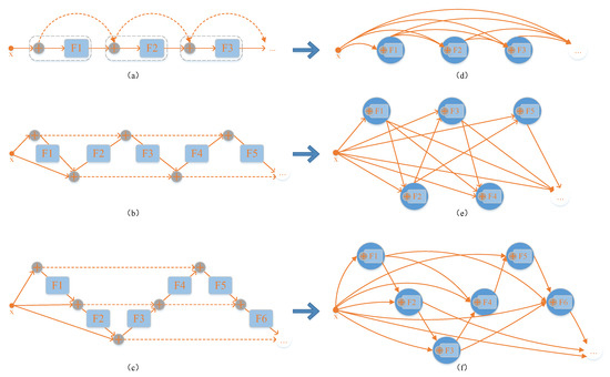
Figure 1. Three examples of mapping from neural networks to directed acyclic graphs. (a) Traditional residual neural network FoldNet_1. (d) Directed acyclic graph mapped from FoldNet_1. (b) Improved folded residual neural network FoldNet_2. (e) Directed acyclic graph mapped from FoldNet_2. (c) Improved folded residual neural network FoldNet_3. (f) Directed acyclic graph mapped from FoldNet_3. In (a–c), the F_i nodes represent nonlinear transformations between data; the circles with plus signs inside represent the summation of all input data. In (d–f), the nodes are composed of summation and nonlinear transformation; the lines indicate the data flow between nodes.

3.2. Improving the Incoherence of DAGs by Folding Residual Networks

In traditional residual neural networks, all jump connections are restricted to adjacent layers, and the distance between any two layers is always equal to 1, which limits the representational power of the network. The residual neural network folds the backbone chain back and forward into an accordion-like structure, as shown in Figure 1b,c.

The improved accordion-like structure is superior to the chain-like structure of the traditional residual neural network in terms of two features. First, the number of direct paths is increased from one to multiple. Second, the distances between layers connected by jump connections are different from each other. These two features are determined by the so-called “folding length”; we named the folding neural network FoldNet-d, where d is the “folding length”. In FoldNet-d networks, d represents the number of direct paths, and the distance of jump connections is an integer in the set [2, 4,…, 2(d − 1)]. When d = 1, the model degenerates to a traditional residual neural network. Figure 1a–c describes the network architectures of FoldNet-1, FoldNet-2, and FoldNet-3, respectively, while Figure 1d–f describes the directed acyclic graphs mapped from FoldNet-1, FoldNet-2, and FoldNet-3, respectively.

The directed acyclic graphs with n nodes mapped from neural networks can be formally represented by an n × n adjacency matrix A, in which element $a_{ij}=1$ if a directed edge from node i to node j exists, and element $a_{ij}=0$ if not. The incoming and outgoing degrees of node i are $k_i^{in}={{\displaystyle \sum }}_j{a}_{ji}$ and $k_i^{out}={{\displaystyle \sum }}_j{a}_{ij}$, respectively. The first node (i = 1) can never have inward edges, so $k_1^{in}=0$. Analogously, the last node (i = n) can never have outward edges, so $k_n^{out}=0$. The trophic level $s_i$ of node i is defined by Equation (1).

$$s_i=1+\frac{1}{k_i^{in}}{{\displaystyle \sum }}_j{a}_{ji}{s}_j$$

(1)

We define the trophic distance from node i to node j as $x_{ij}=s_i-s_j$ if an edge exists from node i to node j. Then, we study the distribution of trophic distances p(x) over directed acyclic graphs. The homogeneity of p(x) is generally referred to as trophic coherence: the closer the trophic distances of all edges, the higher the coherence of the graph. The degree of coherence is usually measured using the standard deviation of p(x), which is named as the incoherence parameter: $q=\sqrt{{\mathit{x}}^2-1}$.

We map the architecture of the neural network into a directed acyclic graph and use the incoherence parameter q to measure the degree of order of the directed acyclic graph. According to the main plot in Figure 2, the incoherence parameter q increases along with the number of nodes (i.e., the layers of the neural network) and the fold length d in the directed acyclic graph. The inset subplot in Figure 2 shows the cumulative distribution function (CDF) of path lengths in the directed acyclic graph when the number of nodes is equal to 50, where the proportion of shorter paths grows as the fold length d increases.

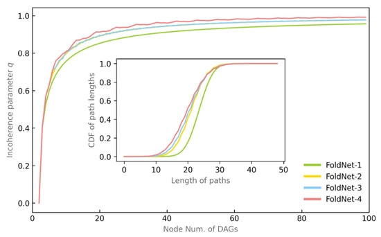
Figure 2. Incoherence and path length of DAG. The main plot demonstrates the relationship between the incoherence parameter q and the number of DAG nodes and the folding length d. The inset subplot illustrates the relationship between the path length and the folding length d.

By comparing the incoherence and path length of the FoldNet-d neural networks with d ∈ [2–4] and the conventional residual neural network at d = 1, we argue that the disorder of the folded residual network FoldNet-d is higher, and the shorter paths account for a larger proportion, thus improving the performance of the FoldNet-d network.

3.3. Model Architecture

Isotropic CNNs emerged partially inspired by the state-of-the-art attention-based transformer architectures in computer vision that are isotropic architectures. Compared to pyramidical architectures, recent research discovered that isotropic architectures may improve performance or even meet state-of-the-art performance with reduced layers. This study designs a lightweight deep isotropic neural network model, FoldNet, which has the same size and shape for all layers throughout the network. In this network model architecture, images are first segmented into a series of patches, and then these patches are passed to a repeating block chain, which is eventually used for automatic identification and classification of plant disease images. Compared to traditional residual neural networks with only one direct path, FoldNet has multiple direct paths throughout the network; therefore, the model can explore deeper into the network and identify plant pest and disease characteristics more accurately.

The FoldNet model architecture is shown in Figure 3a, consisting of a patch embedding layer, repeatedly applied folding blocks, a global average pooling layer, and a classifier block. The patch embedding layer can be implemented by a convolutional operation with three input channels, h output channels, and the same kernel size and stride size p. Each folding block contains d − 1 nonlinear transformations F_i, as shown by the red dashed, rounded rectangles in Figure 3a. Each nonlinear transformation F_i itself consists of a depth-wise convolution and a point-wise convolution, each followed with a GELU activation function and a batch normalization layer, as illustrated in Figure 3b. The depth-wise convolution is a grouped convolution with kernel size k, and the number of groups equal to the number of channels h. The point-wise convolution is a full convolution with a 1 × 1 kernel. Finally, a global average pooling layer is used to obtain the feature vector, which is then passed to a linear classifier and a SoftMax function to predict the probability of all classes.

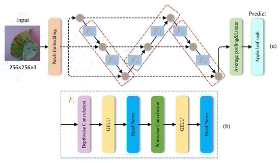
Figure 3. (a) The model architecture of FoldNet, which starts with a patch embedding layer, followed by a series of folded blocks shown by red dashed rectangles, then a pooling layer and a linear classifier, and finally a prediction class where the depth n = 6, the folding length d = 3, and the number of folding blocks is equal to n/(d − 1) = 3. (b) Specific details of each nonlinear transform F_i, including a depth-wise convolution and a point-wise convolution, each followed by a Gaussian error linear unit (GELU) activation function and a batch normalization layer.

4. Materials and Methods

4.1. Image Acquisition

In order to design an efficient and accurate automatic plant disease identification method, our proposed network architecture model was trained and validated on two public datasets, which are summarized in Table 1.

Table 1. Overview of the PlantVillage and FGVC8 datasets.

Dataset	Class	Samples in Training Sets	Samples in Validation Sets
PlantVillage	38	43,444	10,861
FGVC8	12	14,905	3727

The first PlantVillage dataset is a collection of 54,305 images of 14 different plant species belonging to 38 classes, 12 of which are healthy, 26 of which are diseased. The dataset was created by the Penn State College of Agricultural Sciences and the International Institute of Tropical Agriculture as a resource for research and development of computer-vision-based plant disease detection systems. The images in the dataset were collected from various sources, including research institutions and citizen scientists, and represent a wide variety of plant species and disease types. The plants include fruits such as apple, blueberry, cherry, grape, orange, peach, raspberry, squash, and strawberry, crops such as corn and soybean, and vegetables such as bell pepper, potato, and tomato. Each plant has a healthy status or has a disease such as scab, rot, rust, and so on. In addition, the distribution of images of the 38 classes is not uniform, so this unbalanced distribution makes the classification task more challenging and more difficult in terms of training compared to a balanced dataset. Figure 4 shows the unbalanced distribution of the number of images. Figure 5 shows sample images of plant diseases for the 38 classes that appear in the public PlantVillage dataset.

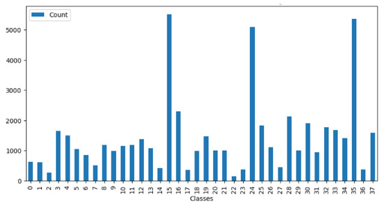
Figure 4. Imbalanced distribution of the counts of images in the PlantVillage dataset.

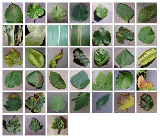
Figure 5. Sample images of plant diseases of 38 classes in the PlantVillage dataset.

The second FGVC8 dataset was provided by the Kaggle Phytopathology 2021-FGVC8 Challenge and has a total of 18,632 plant disease images belonging to 12 categories, all 4000 × 2672 pixels in size. This dataset reflects real field scenarios by representing leaf images with non-homogeneous backgrounds taken at different maturity stages and at different times of day under different focal camera settings. Figure 6 and Figure 7 show the imbalance distribution map of the FGVC8 public dataset and sample images of plant diseases for the 12 classes, respectively.

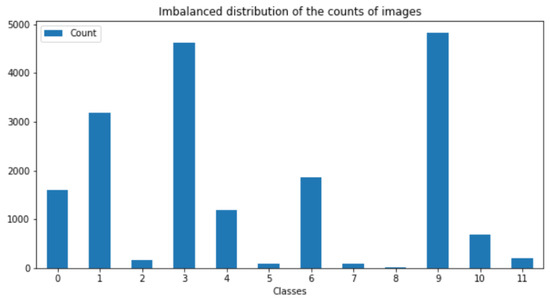
Figure 6. Imbalanced distribution of the counts of images.

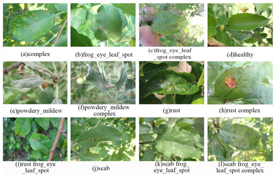
Figure 7. Sample images of plant diseases in the FGVC8 dataset.

4.2. Image Preprocessing and Sample Augmentation Technique

First, all the images in the two datasets were rescaled to 256 × 256 pixels using the resize method in the transforms module of the torchvision package. Then, they were divided into a training set and validation set according to the ratio of 8:2. After that, an online data enhancement method was adopted, and RandomHorizontalFlip, RandomVerticalFlip, RandAugment [35], and ColorJitter methods in the transforms module of the torchvision package were used to perform fast data enhancement operations on data images. By enhancing the image data for the training set, it expands the scale of the dataset, increases the diversity of data samples, reduces the risk of model overfitting, and improves the generalization ability and robustness of the model. Figure 8 shows examples of the original images and the corresponding data-enhanced images.

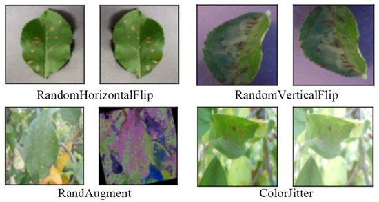
Figure 8. Examples of original images and corresponding data-enhanced images.

4.3. Optimization Method and Loss Function

For this research, we used the AdamW [36] optimization algorithm, which is based on Adam with the addition of the L2 regular term to solve some problems of Adam by weights decays. The AdamW optimization algorithm has several advantages compared with Adam. First, the size of the weights can be better controlled while maintaining the stability of the gradient by adding the L2 regular term. Second, the risk of overfitting can be effectively reduced, thus improving the generalization ability of the model. Finally, AdamW has a better performance when dealing with large-scale datasets.

The main goal of the optimization algorithm is to update the weights at each stage in order to achieve the effect of optimizing the model. The learning rate is one of the most important hyperparameters for training neural networks. If the learning rate is too large, the model will be difficult to converge, and if it is too small, the convergence rate will be too slow, so a reasonable learning rate is necessary for the model to converge to the minimum point instead of the local optimum point or saddle point.

The loss function is commonly used to measure the goodness of a model, that is, to express the degree of gap between the predicted and actual values. When dealing with classification problems, the cross-entropy loss function is usually used to assess the difference between the estimated and actual values. The cross-entropy loss function portrays the distance between two probability distributions, and the smaller the value of the cross-entropy loss, the better the model prediction. The cross-entropy loss function L is defined in Equation (2), where y and $\widehat{y}$ are the observed labels and estimated labels, respectively; o is the outputs of the neural networks that are often are called logits.

$$L\left(\mathit{y},\widehat{\mathit{y}}\right)=-{{\displaystyle \sum }}_{i=1}^n{\mathit{y}}_i\log \frac{\exp ({\mathit{o}}_i)}{{{\displaystyle \sum }}_{j=1}^n\exp ({\mathit{o}}_j)}$$

(2)

4.4. Experimental Configuration and Hyperparameter Setting

In the experiments, the FoldNet model was implemented using Python programming language and PyTorch deep learning framework and was trained and evaluated using PyTorch Lightning library. In addition, due to the limited experimental conditions, we used the online services from Kaggle.com and the PaperSpace.com to provide GPUs for training and evaluation of the models. Kaggle Kernels offers T4 × 2 GPUs that allow each user 30 h of free access per week with a limit of 9 h per run. PaperSpace.com offers a more powerful and faster paid A4000 GPU, but it has a maximum run-time limit of 6 h per run. The software and hardware configurations are shown in Table 2.

Table 2. Software and hardware environment.

Name	PaperSpace	Kaggle
CPU	8 cores	2 cores
GPU	A-4000	T4 × 2
RAM	45 GB	13 GB
CUDA	11.6	11.4
Python	3.9	3.7.12
PyTorch	1.12	1.13
PyTorch Lightning	1.8.0	1.9.4

FoldNet was designed by changing the connectivity method of skip connections between the layers in the residual neural network, which is a macro design methodology. Therefore, we focused on the depth n and the fold length d of the model, which reflect macro structural features of the model. Meanwhile, we kept the values of the patch size p and the kernel size k fixed, which reflects the micro design features of the model. According to the suggestion in the ConvMixer [37] model, we set the patch size p = 8 and the kernel size k = 5.

The FoldNet model has slightly different hyperparameter settings for different datasets. For the PlantVillage dataset, we trained FoldNet for 100 epochs with a batch size of 128 and utilized the AdamW optimizer with a learning rate of 0.01 and a weight decay of 0.1. There was a linear warm up of 10 epochs with an initial learning rate of 0.00001 followed by a cosine decay schedule. For the FGVC8 dataset, FoldNet was also trained for 100 epochs but with a batch size of 64, also utilizing the AdamW optimizer with a learning rate of 0.01 but with a weight decay of 0.05, where there was also a linear warm up of 10 epochs with an initial learning rate of 0.00001 followed by a cosine decay schedule.

4.5. Evaluation Metrics

In the experiments, we used accuracy, precision, recall, and F1-score as evaluation metrics to make a comprehensive assessment of model performance. We usually use the following metrics to obtain evaluation results: If an instance is a positive class and is predicted to be a positive class, it is a true-positive class TP (True Positive); if an instance is a positive class but is predicted to be a negative class, it is a false-negative class FN (False Negative); if an instance is a negative class but is predicted to be a positive class, it is a false-positive class FP (False Positive); if an instance is a negative class and is predicted to be a negative class, it is a true-negative class TN (True Negative). T/F represents the correctness or incorrectness of the prediction, and P/N represents the positive or negative case of the prediction result. The accuracy rate is the proportion of correctly predicted samples to the total samples, which reflects the overall performance of the model and is often expressed as in Equation (3). The precision rate is the proportion of samples both predicted to be positive and actually positive to those predicted to be positive and is often expressed as in Equation (4). Recall is the proportion of predicted positive and actual positive samples to the actual positive samples and is often expressed as in Equation (5). In order to obtain a balance between precision and recall, the F1-score metric is used, which is the summed average of precision and recall, and this score considers both false positives and false negatives; moreover, a higher F1-score indicates better model performance, which is often expressed as in Equation (6).

$$\mathrm{Accuracy}=\frac{TP+TN}{TP+TN+FP+FN}$$

(3)

$$\mathrm{Precision}=\frac{TP}{TP+FP}$$

(4)

$$\mathrm{Recall}=\frac{TP}{TP+FN}$$

(5)

$$\mathrm{F}1\mathrm{score}=\frac{2precision\ast recall}{precision+recall}$$

(6)

5. Results and Discussion

5.1. Experimental Results with Different Hyperparameter Values

Since the effect of depth n and fold length d on the performance of the FoldNet model was orthogonal to the hidden dimension h, we conducted experiments for hidden dimension h = 64 and h = 128, respectively, to compare the performance of the model for plant disease recognition under different hyperparameters.

For the PlantVillage dataset, the experimental results of the FoldNet model are shown in Table 3, with a total of 24 items. Through the experiments, our model obtained optimal results at epoch = 98 when the hidden dimension h = 128. In detail, our model achieved the best validation accuracy of 0.9984 and the lowest validation loss of 0.0039 on the PlantVillage validation set, while the number of model parameters was only 685k, which proves the effectiveness and robustness of the proposed model. As shown in Table 3, from an overall perspective, FoldNet_2, FoldNet_3, and FoldNet_4 with d > 1 outperformed FoldNet_1 with d = 1 on the PlantVillage dataset. In addition, when the hidden dimension h = 128, the validation accuracy of all FoldNet models at the corresponding depth n was higher than that at the hidden dimension h = 64, and the validation loss of all FoldNet models at the corresponding depth n was lower than that at the hidden dimension h = 64. Moreover, FoldNet_2 with d > 1 obtained the highest validation accuracy at depth n = 32 when the hidden dimension h = 128. Compared with FoldNet_1 with h = 128, FoldNet_2 improved the validation accuracy by 0.1% at the same depth n = 32, and its validation loss was reduced by 0.88%. Compared with FoldNet_2 with h = 64, FoldNet_2 with h = 128 improved the validation accuracy by 0.1%, and its validation loss was reduced by 0.61% at the same depth n = 32.

Table 3. Validation accuracy and validation loss of FoldNet-d (d = 1, 2, 3, 4) for the PlantVillage dataset with hidden dimension h = 64 and h = 128. The depth n is calculated by the number of folding blocks times d − 1. The patch size p and kernel size k are fixed as p = 8 and k = 5.

FoldNet-d	Depth n	h = 64	h = 128	h = 64	h = 128
		Val. Accuracy		Val. Loss
FoldNet-1	16	0.9960	0.9974	0.0114	0.0092
	24	0.9959	0.9976	0.0128	0.0085
	32	0.9958	0.9974	0.0144	0.0127
	40	0.9962	0.9968	0.0142	0.0105
	48	0.9960	0.9976	0.0171	0.0110
FoldNet-2	16	0.9961	0.9976	0.0162	0.0071
	24	0.9961	0.9980	0.0150	0.0062
	32	0.9974	0.9984	0.0100	0.0039
	40	0.9975	0.9977	0.0094	0.0078
	48	0.9975	0.9983	0.0101	0.0084
FoldNet-3	16	0.9971	0.9978	0.0115	0.0105
	18	0.9970	0.9981	0.0115	0.0097
	24	0.9976	0.9983	0.0102	0.0053
	26	0.9967	0.9982	0.0128	0.0075
	32	0.9964	0.9981	0.0128	0.0097
	34	0.9968	0.9981	0.0118	0.0087
	48	0.9972	0.9979	0.0109	0.0072
FoldNet-4	15	0.9966	0.9982	0.0125	0.0066
	21	0.9969	0.9980	0.0106	0.0077
	27	0.9970	0.9981	0.0099	0.0075
	33	0.9971	0.9980	0.0148	0.0081
	39	0.9973	0.9981	0.0131	0.0063
	45	0.9972	0.9981	0.0141	0.0094
	48	0.9975	0.9983	0.0119	0.0088

For the realistic scene dataset FGVC8, the experimental results of the FoldNet model under this dataset are shown in Table 4, with a total of 24 items. Through the experiments, our model obtained optimal results at epoch = 81 when the hidden dimension h = 128. In detail, our model achieved the highest validation accuracy of 0.9049 and low validation loss of 0.3789 on the validation set of FGVC8, while the number of model parameters was only 516k, which, again, demonstrates the effectiveness and robustness of the proposed model. As shown in Table 4, from an overall perspective, FoldNet_2, FoldNet_3, and FoldNet_4 with d > 1 outperformed FoldNet_1 with d = 1 on the PlantVillage dataset. In addition, when the hidden dimension h = 128, the validation accuracy of all FoldNet models at the corresponding depth n was higher than that at the hidden dimension h = 64, and the validation loss of all FoldNet models at the corresponding depth n was lower than that at the hidden dimension h = 64. In addition, when the hidden dimension h = 128, FoldNet_2 with d > 1 obtained the highest validation accuracy at depth n = 24. Compared with FoldNet_1 with h = 128, FoldNet_2 improved the validation accuracy by 2.52% at the same depth n = 24, and its validation loss was reduced by 2.13%. Compared with FoldNet_2 with h = 64, FoldNet_2 with h = 128 improved the validation accuracy by 2.92%, and its validation loss was reduced by 2.9% at the same depth n = 24.

Table 4. Validation accuracy and validation loss of FoldNet-d (d = 1, 2, 3, 4) for the FGVC8 dataset with hidden dimension h = 64 and h = 128. The depth n is calculated by the number of folding blocks times d − 1. The patch size p and kernel size k are fixed as p = 8 and k = 5.

FoldNet-d	Depth n	h = 64	h = 128	h = 64	h = 128
		Val. Accuracy		Val. Loss
FoldNet-1	16	0.8714	0.8792	0.4151	0.3947
	24	0.8703	0.8797	0.4027	0.4002
	32	0.8696	0.8730	0.4076	0.3982
	40	0.8669	0.8792	0.4200	0.4186
	48	0.8687	0.8790	0.4022	0.3929
FoldNet-2	16	0.8804	0.8866	0.3857	0.3733
	24	0.8757	0.9049	0.4079	0.3789
	32	0.8787	0.8879	0.4182	0.3959
	40	0.8714	0.8870	0.4080	0.4065
	48	0.8719	0.8846	0.4082	0.4065
FoldNet-3	16	0.8681	0.8910	0.4053	0.3981
	18	0.8828	0.8836	0.3879	0.3850
	24	0.8706	0.8807	0.4079	0.3957
	26	0.8787	0.8801	0.4031	0.3995
	32	0.8736	0.8900	0.4105	0.3857
	34	0.8810	0.8834	0.4023	0.3987
	48	0.8745	0.8801	0.4143	0.4009
FoldNet-4	15	0.8774	0.8856	0.3945	0.3850
	21	0.8774	0.8887	0.4332	0.3868
	27	0.8792	0.8821	0.4113	0.4084
	33	0.8743	0.8875	0.4012	0.3700
	39	0.8768	0.8822	0.4050	0.4011
	45	0.8836	0.8950	0.3958	0.3946
	48	0.8793	0.8880	0.4003	0.3968

5.2. Confusion Matrix Analysis

To validate the success of the FoldNet network model for plant disease classification, we used confusion matrices to evaluate the classification performance of the model. The confusion matrix is a visualization tool in machine learning which is a table layout that compares the predicted class labels with the actual class labels for all data instances. The rows of the matrix represent the actual classes, while the columns represent the predicted classes. By analyzing the confusion matrix, we can determine how well the model is able to distinguish between different classes, as well as which classes are most often confused with one another. Popular performance metrics, such as accuracy, precision, recall, F1-score can be derived from the confusion matrix.

The PlantVillage dataset has a tree-like hierarchical structure with three levels. The root node is the overall category, plant. The first level is the 14 specific plant species. The second level is the healthy or disease status of the plant. Thus, we used a hierarchical confusion matrix to evaluate the model on the 10,861 validation images in the PlantVillage dataset. The precision, recall, and F1-scores for each category in the PlantVillage dataset are shown in Table 5. Due to the imbalance in numbers between categories in the PlantVillage dataset, we used micro-averages to calculate the overall metrics. The micro-averages of precision, recall, and F1-scores were 0.9984, 0.9984, and 0.9984.

Table 5. Performance evaluation on the PlantVillage for each class.

Plant	Disease	Class Labels	Precision	Recall	F1-Score
Apple	Healthy	0	1.00	1.00	1.00
	Scab	1	1.00	1.00	1.00
	Black Rot	2	1.00	1.00	1.00
	Cedar Rust	3	1.00	1.00	1.00
Blueberry	Healthy	4	1.00	1.00	1.00
Cherry	Healthy	5	1.00	0.9883	0.9941
	Powdery Mildew	6	1.00	1.00	1.00
Corn	Healthy	7	1.00	1.00	1.00
	Cercospora Leaf Spot	8	0.9736	0.9910	0.9823
	Common Rust	9	1.00	0.9956	0.9978
	Northern Leaf Blight	10	0.9951	0.9903	0.9927
Grape	Healthy	11	1.00	1.00	1.00
	Black Rot	12	1.00	1.00	1.00
	Black Measles	13	1.00	1.00	1.00
	Isariopsis Leaf Spot	14	1.00	1.00	1.00
Orange	Citrus Greening	15	1.00	0.9990	0.9995
Peach	Healthy	16	1.00	1.00	1.00
	Bacterial Spot	17	1.00	1.00	1.00
Bell Pepper	Healthy	18	1.00	1.00	1.00
	Bacterial Spot	19	0.9952	1.00	0.9976
Potato	Healthy	20	1.00	1.00	1.00
	Early Blight	21	1.00	1.00	1.00
	Late Blight	22	1.00	1.00	1.00
Raspberry	Healthy	23	1.00	1.00	1.00
Soybean	Healthy	24	0.9989	1.00	0.9994
Squash	Powdery Mildew	25	0.9971	1.00	0.9985
Strawberry	Healthy	26	1.00	1.00	1.00
	Leaf Scorch	27	0.9949	1.00	0.9974
Tomato	Healthy	28	0.9965	1.00	0.9982
	Bacterial Spot	29	0.9951	1.00	0.9975
	Early Blight	30	0.9951	0.9857	0.9904
	Late Blight	31	0.9951	0.9927	0.9939
	Leaf Mold	32	1.00	1.00	1.00
	Septoria Leaf Spot	33	0.9972	1.00	0.9986
	Spider Mites	34	0.9936	1.00	0.9968
	Target Spot	35	1.00	0.9966	0.9983
	Yellow Leaf Curl	36	1.00	0.9972	0.9986
	Mosaic Virus	37	1.00	1.00	1.00
	Micro-Average		0.9984	0.9984	0.9984

The FoldNet model achieved 99.84% accuracy on the PlantVillage dataset, and, as can observed from the confusion matrix shown in Figure 9, the proposed FoldNet method had fewer false positives and false negatives on the PlantVillage dataset, and only 17 images in this dataset were misclassified. After quantitatively analyzing these 17 images, we found three interesting points which needed to be noted: First, compared to incorrect classification within the same species, incorrect classification across species was very rare. Only five images were incorrectly identified as images of different plant species, as shown in Figure 10, while the other 12 images were identified correctly by species, as shown in Figure 11, even though they were identified incorrectly in terms of their disease status. This reflects the robustness of the FoldNet model, which can correctly predict the species of an image even if its prediction of the image’s disease status is wrong. Second, the 12 images that were incorrectly classified within the same species belonged to two species, corn and tomato, rather than being uniformly distributed across all the 14 species. Of the 12 images, 4 belonged to corn, and the other 8 images belonged to tomato. This reflects the complexity of the images of corn and tomato. Third, in the 17 images that were classified incorrectly, several images were wrong in ground truth or captured in an extreme situation. For example, the first ‘Cherry Healthy’ image was actually a field background; two “Tomato Late Blight” images had a very small foreground and a very large background.

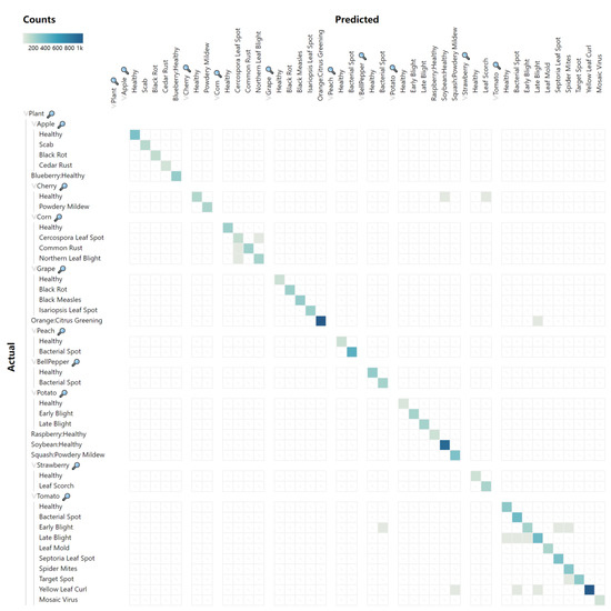
Figure 9. Confusion matrix of FoldNet for the PlantVillage dataset.

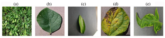
Figure 10. The 5 images that are incorrectly predicted as images of other plant species. (a) Actual: Cherry Healthy, predicted: Soybean Healthy; (b) actual: Cherry Healthy, predicted: Strawberry Leaf Scorch; (c) actual: Orange Citrus Greening, predicted: Tomato Late Blight; (d) actual: Tomato Early Blight, predicted: Bell Pepper Bacterial Spot; (e) actual: Tomato Yellow Leaf Curl, predicted: Squash Powdery Mildew.

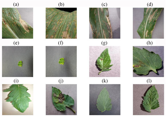
Figure 11. The 12 images with correctly predicted species, but incorrectly predicted disease state. (a) Actual: Corn Cercospora Leaf Spot, predicted: Corn Northern Leaf Blight; (b) actual: Corn Common Rust, predicted: Corn Cercospora Leaf Spot; (c) actual: Corn Northern Leaf Blight, predicted: Corn Cercospora Leaf Spot; (d) actual: Corn Northern Leaf Blight, predicted: Corn Cercospora Leaf Spot; (e) actual: Tomato Yellow Leaf Curl, predicted: Tomato Late Blight; (f) actual: Tomato Yellow Leaf Curl, predicted: Tomato Bacterial Spot; (g) actual: Tomato Early Blight, predicted: Tomato Spider Mites; (h) actual: Tomato Early Blight, predicted: Tomato Septoria Leaf Spot; (i) actual: Tomato Late Blight, predicted: Tomato Bacterial Spot; (j) actual: Tomato Late Blight, predicted: Tomato Early Blight; (k) actual: Tomato Late Blight, predicted: Tomato Healthy; (l) actual: Tomato Target Spot, predicted: Tomato Spider Mites.

For the FGVC8 apple leaf disease dataset, we still chose the hierarchical confusion matrix to evaluate the model for the 3727 validation images in the FGVC8 dataset. The precision, recall, and F1-scores for each category in the FGVC8 dataset are shown in Table 6. Since the number of categories in the FGVC8 dataset is unbalanced, we used micro-averages to calculate the overall metrics. The micro-averages of precision, recall, and F1-score were 0.9049, 0.9049, and 0.9049.

Table 6. Performance evaluation on the FGVC8 for each class.

Plant	Disease	Class Labels	Precision	Recall	F1-Score
Apple	Complex	0	0.7071	0.7376	0.7220
	Frogeye Leaf Spot	1	0.9007	0.9696	0.9339
	Frogeye Leaf Spot Complex	2	0.6666	0.3636	0.4705
	Healthy	3	0.9572	0.9828	0.9698
	Powdery Mildew	4	0.9288	0.9406	0.9347
	Powdery Mildew Complex	5	0.75	0.625	0.6818
	Rust	6	0.8968	0.9630	0.9287
	Rust Complex	7	1.00	0.6470	0.7857
	Rust Frogeye Leaf Spot	8	0.7222	0.5	0.5909
	Scab	9	0.9563	0.9457	0.9509
	Scab Frogeye Leaf Spot	10	0.6125	0.4117	0.4924
	Scab Frogeye Leaf Spot Complex	11	0.8571	0.15	0.2553
	Micro-Average		0.9049	0.9049	0.9049

The FoldNet model achieved an accuracy of 90.49% on the FGVC8 dataset. From the observation of the confusion matrix shown in Figure 12, we can obviously see that the proposed FoldNet method had good overall classification performance for the 12 classes in this dataset, but there were still some misclassified samples. Through comparative analysis, firstly, we found that most of the misclassified samples exhibited similar epigenetic characteristics, and, secondly, there were multiple different types of diseases in the complex class of leaf diseases, and these diseases were difficult to distinguish from those in other classes because of their similarity. Figure 13 shows some of the misclassified samples.

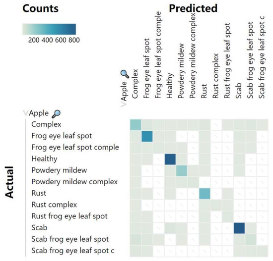
Figure 12. Confusion matrix of FoldNet for the FGVC8 dataset.

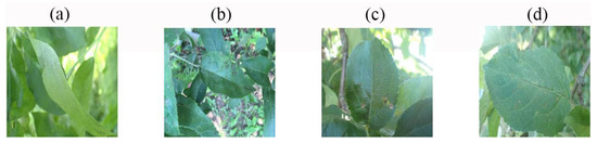
Figure 13. 4 example images of incorrectly predicted disease states. (a) Actual: Powdery Mildew, predicted: Healthy; (b) actual: Rust, predicted: Healthy; (c) actual: Rust Frogeye Leaf Spot, predicted: Complex; (d) actual: Scab Frogeye Leaf Spot Complex, predicted: Scab.

5.3. Qualitative Analysis

GradCAM [38] heat map is a visualization tool used to explain the decision process of a deep learning model. Through GradCAM heat maps, we can analyze the features of the regions that the model focuses on when classifying the input data. We randomly selected three disease samples from each of the PlantVillage and FGVC8 validation datasets and then use GradCAM to visualize the plant disease identification results, where red-highlighted areas indicated areas where the model focused strongly on one category, and blue indicated areas where the model discriminated more strongly between other categories. Figure 14 shows the original map of different plant diseases and the map of plant disease features captured by the proposed method, respectively. After comparison, it was found that the method can clearly discover the location of plant disease regions and gradually enhance the characterization of disease features in the region of interest. In addition, we found that the method is good at capturing plant disease areas and extracting subtle features for both laboratory data and realistic scenarios, thus improving the accurate identification of plant diseases.

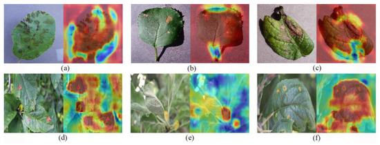
Figure 14. Feature map of different crop diseases. (a) Apple Scab. (b) Black Rot. (c) Potato Late Blight. (d) Apple Rust. (e) Powdery Mildew. (f) Apple Rust.

5.4. Comparison with Other Methods

In this section, we describe an experiment to compare the performance of the proposed method with other methods for disease identification, where all methods used the same experimental methods and experimental environments, and all were performed on the PlantVillage and FGVC8 datasets.

In Table 7 and Table 8 we show the complexity of the model, from which we can obviously see that our proposed method always contained a minimum number of parameters that is fewer than 1M, both for the PlantVillage dataset and for the FGVC8 dataset. In addition, on the PlantVillage dataset, the proposed method spendt the least amount of time compared to the other methods to complete the task of identifying and classifying various plant diseases. On the FGVC8 dataset, the proposed method also took less time than the other methods to perform all operations. More specifically, on the PlantVillage dataset, the VGG16 model contained the largest number of parameters, about 175 times more than the proposed model FoldNet, and ResNet152 was the most resource-consuming method in terms of processing time. However, in contrast, our proposed FoldNet model contained only 685k parameters, which is fewer than any other model, and required only 1010 ms minimum processing time. For the FGVC8 dataset, the Inception-ResNetV2 model contained the largest number of parameters, about 100 times more than the proposed model FoldNet, and PatchConvNet was the most resource-consuming method in terms of processing time. However, in contrast, our proposed FoldNet model contained only 516k parameters, which is fewer than any other model, and required only 3.6 h of minimum operation time. In summary, the effectiveness of the FoldNet model for plant disease identification in controlled environments and realistic scenarios was demonstrated, and, as seen in the comparative analysis of Table 7 and Table 8, our model provides a lightweight solution for plant disease identification.

Table 7. Comparative analysis of the proposed method with other methods on PlantVillage regarding computational complexity.

Model	Parameter	Processing Time
VGG16 [39]	119.6M	1051 ms
ResNet50 (transfer learning) [19]	23.6M	1583 ms
ResNet101	42.5M	2766 ms
ResNet152	58.5M	4366 ms
DenseNet201 [21]	20M	2573 ms
InceptionV4 [40]	41.2M	4042 ms
EfficientNet [41]	19.4M	1548 ms
EfficientNetV2 [42]	15.2M	1125 ms
DenseNet121 (transfer learning) [24]	7.1M	2165 ms
modified EfficientNetV2 [30]	14.4M	1053 ms
Proposed	685k	1010 ms

Table 8. Comparative analysis of the proposed method with other methods on FGVC8 regarding computational complexity.

Model	Parameter	Time
Inception-ResNetV2 [18]	51.83M	4.8 h
SEResNet50 [43]	26.06M	4.1 h
PatchConvNet [44]	24.78M	6.5 h
ResMLP-S12 [45]	14.94M	4.5 h
CoAtNet [46]	16.99M	4.4 h
VAN-B0 [47]	3.85M	3.7 h
DenseNet-MFA [31]	9.45M	4.5 h
Proposed	516k	3.6 h

In Table 9 and Table 10 we demonstrate the performance of the proposed method compared with other methods in terms of average accuracy, average precision, average recall, and average F1-score. It can be seen that, for PlantVillage, our model achieved more advanced results in terms of average accuracy, average precision, average recall, and average F1-score compared to other methods. In detail, the average accuracy was 2.74–0.9% higher, the average precision was 8.84–0.49% higher, the average recall was 6.84–0.49% higher, and the average F1-score was 7.84–0.5% higher. The excellent performance demonstrated the plant disease identification ability of the proposed model. It can be seen for FGVC8 that our model achieved equally good results in recognizing plant disease images of realistic scenes. Compared with other methods, the average accuracy was 11.59–0.54% higher, the average precision was 10.43–1.45% higher, the average F1-score was 9.5–0.49% higher, and the average recall achieved optimal results like those of other methods, all of which indicate the excellent robustness of our model. Most importantly, our proposed model FoldNet had only 516k parameters, which is lower than all other models, and required only 3.6 h minimum operation time. This means it is possible to train and deploy the model faster, which is important in real-time applications. Furthermore, the technology can be easily ported to mobile or embedded devices, which offers tremendous promise for precision agriculture development.

Table 9. Average values of deep-learning-based methods on PlantVillage dataset.

Model	Accuracy	Precision	Recall	F1-Score
ResNet50	0.982	0.94	0.94	0.94
DenseNet169	0.974	0.92	0.93	0.93
AlexNet (transfer learning) [22]	0.9928	0.9928	0.9927	0.9927
AlexNet (trained from scratch)	0.9782	0.9786	0.9782	0.9782
GoogleNet (transfer learning) [22]	0.9935	0.9935	0.9935	0.9934
GoogleNet (training from scratch)	0.9837	0.9839	0.9837	0.9836
DenseNet121 (transfer learning)	0.9975	-	-	-
MobileNet [20]	0.971	0.94	0.93	9.93
InceptionV3 [17]	0.971	0.92	0.94	0.93
Inception-ResNetV2	0.978	0.91	0.93	0.92
Module 4 [34]	-	0.9878	0.9877	0.9877
Proposed	0.9984	0.9984	0.9984	0.9984

Table 10. Average values of deep-learning-based methods on the FGVC8.

Model	Accuracy	Precision	Recall	F1-Score
ResNet50	0.8664	0.8534	0.8664	0.8599
ResNet152	0.789	-	-	-
VGG16	0.83	-	-	-
DenseNet121	0.8704	0.8679	0.8704	0.8691
InceptionV3	0.803	-	-	-
MobileNetV2 [42]	0.8521	0.8513	0.8521	0.8517
Inception-ResNetV2	0.8590	0.8630	0.8590	0.8610
SEResNet50	0.8657	0.8504	0.8657	0.8580
PatchConvNet	0.8196	0.8007	0.8196	0.8100
ResMLP-S12	0.8535	0.8417	0.8535	0.8476
CoAtNet	0.8743	0.8653	0.8743	0.8698
VAN-B0	0.8853	0.8863	0.8853	0.8856
DenseNet-MFA	0.8995	0.8854	0.8995	0.8924
MobileNet + Xception + InceptionResNet [48]	0.8731	0.8905	0.9100	0.9001
Proposed	0.9049	0.9049	0.9049	0.9049

6. Conclusions

In this study, we designed a lightweight deep isotropic neural network model, FoldNet, to recognize plant disease images in controlled environments and realistic scenes. Within this network model architecture, images are first segmented into a series of patches, which are then passed to a repeating chain of blocks for automatic identification and classification of plant disease images. The proposed model has the same size and shape for all layers in the whole network, which is achieved by folding the same block chains and then connecting the blocks with skip connections at different distances. The model has multiple directly connected paths in the whole network, can explore deeper layers, and thus can identify the plant disease characteristics more accurately. Additionally, we used image preprocessing techniques and sample-enhancement techniques to increase the size of the dataset and improve the generalization of the model.

We evaluated the recognition performance of FoldNet for plant disease images of the PlantVillage and FGVC8 datasets by adjusting its width h, depth n, and fold length d. We found that the accuracy of FoldNet was positively correlated with its depth n and fold length d, and it achieved the best recognition performance for the PlantVillage and FGVC8 datasets when the width h equaled 128. Compared with several other state-of-the-art models, FoldNet achieved competitive classification accuracy on the PlantVillage and FGVC8 datasets with fewer parameters and less computational time. In summary, FoldNet provides a lightweight, low-cost solution for plant disease identification oriented to realistic scenarios.

Although our model can effectively capture minute features of plant diseases and enhance the ability to characterize diseases, there are still many aspects that can be improved. To further improve the performance of the model, we plan to collect more realistic scenario data of different types, parts, and stages of plant diseases in future work and develop more efficient and accurate deep learning models that can not only distinguish multiple types of plant diseases but also determine the stages of plant disease occurrence.

References

- Golhani, K.; Balasundram, S.K.; Vadamalai, G.; Pradhan, B. A review of neural networks in plant disease detection using hyperspectral data. Inf. Process. Agric. 2018, 5, 354–371. [Google Scholar] [CrossRef]
- Shruthi, U.; Nagaveni, V.; Raghavendra, B. A review on machine learning classification techniques for plant disease detection. In Proceedings of the 2019 5th International Conference on Advanced Computing & Communication Systems (ICACCS), Coimbatore, India, 15–16 March 2019; pp. 281–284. [Google Scholar]
- Sethy, P.K.; Barpanda, N.K.; Rath, A.K.; Behera, S.K. Deep feature based rice leaf disease identification using support vector machine. Comput. Electron. Agric. 2020, 175, 105527. [Google Scholar] [CrossRef]
- Vaswani, A.; Shazeer, N.; Parmar, N.; Uszkoreit, J.; Jones, L.; Gomez, A.N.; Kaiser, Ł.; Polosukhin, I. Attention is all you need. Adv. Neural Inf. Process. Syst. 2017, 30, 5998–6008. [Google Scholar]
- Cambria, E.; White, B. Jumping NLP curves: A review of natural language processing research. IEEE Comput. Intell. Mag. 2014, 9, 48–57. [Google Scholar] [CrossRef]
- Dosovitskiy, A.; Beyer, L.; Kolesnikov, A.; Weissenborn, D.; Zhai, X.; Unterthiner, T.; Dehghani, M.; Minderer, M.; Heigold, G.; Gelly, S. An image is worth 16 × 16 words: Transformers for image recognition at scale. arXiv 2020, arXiv:2010.11929. [Google Scholar]
- Feng, W.; Zhang, X.; Song, Q.; Sun, G. The Incoherence of Deep Isotropic Neural Networks Increases Their Performance in Image Classification. Electronics 2022, 11, 3603. [Google Scholar] [CrossRef]
- Bao, W.; Yang, X.; Liang, D.; Hu, G.; Yang, X. Lightweight convolutional neural network model for field wheat ear disease identification. Comput. Electron. Agric. 2021, 189, 106367. [Google Scholar] [CrossRef]
- Islam, M.; Anh, D.; Wahid, K.; Bhowmik, P. Detection of potato diseases using image segmentation and multiclass support vector machine. In Proceedings of the 2017 IEEE 30th Canadian Conference on Electrical and Computer Engineering (CCECE), Windsor, ON, Canada, 30 April–3 May 2017; pp. 1–4. [Google Scholar]
- Agrawal, N.; Singhai, J.; Agarwal, D.K. Grape leaf disease detection and classification using multi-class support vector machine. In Proceedings of the 2017 International Conference on Recent Innovations in Signal processing and Embedded Systems (RISE), Bhopal, India, 27–29 October 2017; pp. 238–244. [Google Scholar]
- Dhakate, M.; Ingole, A.B. Diagnosis of pomegranate plant diseases using neural network. In Proceedings of the 2015 Fifth National Conference on Computer Vision, Pattern Recognition, Image Processing and Graphics (NCVPRIPG), Patna, India, 16–19 December 2015; pp. 1–4. [Google Scholar]
- Al-Hiary, H.; Bani-Ahmad, S.; Ryalat, M.; Braik, M.; Alrahamneh, Z. Fast and Accurate Detection and Classification of Plant Diseases. Int. J. Comput. Appl. 2011, 17, 31–38. [Google Scholar] [CrossRef]
- Kaushal, G.; Bala, R. GLCM and KNN based algorithm for plant disease detection. Int. J. Adv. Res. Electr. Electron. Instrum. Eng. 2017, 6, 5845–5852. [Google Scholar]
- Majumdar, D.; Ghosh, A.; Kole, D.K.; Chakraborty, A.; Majumder, D.D. Application of fuzzy c-means clustering method to classify wheat leaf images based on the presence of rust disease. In Proceedings of Proceedings of the 3rd International Conference on Frontiers of Intelligent Computing: Theory and Applications (FICTA), Bhubaneswar, India, 14–15 November 2014; pp. 277–284.
- Weng, Y.; Zeng, R.; Wu, C.M.; Wang, M.; Wang, X.J.; Liu, Y.J. A survey on deep-learning-based plant phenotype research in agriculture (in Chinese). Sci. Sin. Vitae 2019, 49, 698–716. [Google Scholar] [CrossRef]
- Sagar, A.; Jacob, D. On using transfer learning for plant disease detection. BioRxiv 2020, 2020.05. 22.110957. [Google Scholar]
- Szegedy, C.; Vanhoucke, V.; Ioffe, S.; Shlens, J.; Wojna, Z. Rethinking the inception architecture for computer vision. In Proceedings of the IEEE Conference on Computer Vision and Pattern Recognition, Las Vegas, NV, USA, 27–30 June 2016; pp. 2818–2826. [Google Scholar]
- Ai, Y.; Sun, C.; Tie, J.; Cai, X. Research on recognition model of crop diseases and insect pests based on deep learning in harsh environments. IEEE Access 2020, 8, 171686–171693. [Google Scholar] [CrossRef]
- He, K.; Zhang, X.; Ren, S.; Sun, J. Deep residual learning for image recognition. In Proceedings of the IEEE Conference on Computer Vision and Pattern Recognition, Las Vegas, NV, USA, 27–30 June 2016; pp. 770–778. [Google Scholar]
- Howard, A.G.; Zhu, M.; Chen, B.; Kalenichenko, D.; Wang, W.; Weyand, T.; Andreetto, M.; Adam, H. Mobilenets: Efficient convolutional neural networks for mobile vision applications. arXiv 2017, arXiv:1704.04861. [Google Scholar]
- Huang, G.; Liu, Z.; Van Der Maaten, L.; Weinberger, K.Q. Densely connected convolutional networks. In Proceedings of the IEEE Conference on Computer Vision and Pattern Recognition, Honolulu, HI, USA, 21–26 July 2017; pp. 4700–4708. [Google Scholar]
- Mohanty, S.P.; Hughes, D.P.; Salathé, M. Using deep learning for image-based plant disease detection. Front. Plant Sci. 2016, 7, 1419. [Google Scholar] [CrossRef] [PubMed]
- Brahimi, M.; Boukhalfa, K.; Moussaoui, A. Deep learning for tomato diseases: Classification and symptoms visualization. Appl. Artif. Intell. 2017, 31, 299–315. [Google Scholar] [CrossRef]
- Too, E.C.; Yujian, L.; Njuki, S.; Yingchun, L. A comparative study of fine-tuning deep learning models for plant disease identification. Comput. Electron. Agric. 2019, 161, 272–279. [Google Scholar] [CrossRef]
- Rangarajan, A.K.; Whetton, R.L.; Mouazen, A.M. Detection of fusarium head blight in wheat using hyperspectral data and deep learning. Expert Syst. Appl. 2022, 208, 118240. [Google Scholar] [CrossRef]
- Goyal, L.; Sharma, C.M.; Singh, A.; Singh, P.K. Leaf and spike wheat disease detection & classification using an improved deep convolutional architecture. Inform. Med. Unlocked 2021, 25, 100642. [Google Scholar]
- Liu, B.; Zhang, Y.; He, D.; Li, Y. Identification of apple leaf diseases based on deep convolutional neural networks. Symmetry 2017, 10, 11. [Google Scholar] [CrossRef]
- Sun, P.; Chen, G.F.; Cao, L.Y. Image recognition of soybean pests based on attention convolutional neural network (in Chinese). J. Chin. Agric. Mech. 2020, 41, 171–176. [Google Scholar]
- Upadhyay, S.K.; Kumar, A. A novel approach for rice plant diseases classification with deep convolutional neural network. Int. J. Inf. Technol. 2022, 14, 185–199. [Google Scholar] [CrossRef]
- Albattah, W.; Javed, A.; Nawaz, M.; Masood, M.; Albahli, S. Artificial intelligence-based drone system for multiclass plant disease detection using an improved efficient convolutional neural network. Front. Plant Sci. 2022, 13, 808380. [Google Scholar] [CrossRef] [PubMed]
- Zuo, X.; Chu, J.; Shen, J.; Sun, J. Multi-Granularity Feature Aggregation with Self-Attention and Spatial Reasoning for Fine-Grained Crop Disease Classification. Agriculture 2022, 12, 1499. [Google Scholar] [CrossRef]
- Zhong, Y.; Huang, B.; Tang, C. Classification of Cassava Leaf Disease Based on a Non-Balanced Dataset Using Transformer-Embedded ResNet. Agriculture 2022, 12, 1360. [Google Scholar] [CrossRef]
- Guo, Y.; Lan, Y.; Chen, X. CST: Convolutional Swin Transformer for detecting the degree and types of plant diseases. Comput. Electron. Agric. 2022, 202, 107407. [Google Scholar] [CrossRef]
- Borhani, Y.; Khoramdel, J.; Najafi, E. A deep learning based approach for automated plant disease classification using vision transformer. Sci. Rep. 2022, 12, 11554. [Google Scholar] [CrossRef]
- Cubuk, E.D.; Zoph, B.; Shlens, J.; Le, Q.V. Randaugment: Practical automated data augmentation with a reduced search space. In Proceedings of the IEEE/CVF Conference on Computer Vision and Pattern Recognition Workshops, Seattle, WA, USA, 14–19 June 2020; pp. 702–703. [Google Scholar]
- Loshchilov, I.; Hutter, F. Decoupled weight decay regularization. arXiv 2017, arXiv:1711.05101. [Google Scholar]
- Trockman, A.; Kolter, J.Z. Patches are all you need? arXiv 2022, arXiv:2201.09792. [Google Scholar]
- Selvaraju, R.R.; Cogswell, M.; Das, A.; Vedantam, R.; Parikh, D.; Batra, D. Grad-cam: Visual explanations from deep networks via gradient-based locali-zation. In Proceedings of the IEEE International Conference on Computer Vision, Venice, Italy, 22–29 October 2017; pp. 618–626. [Google Scholar]
- Simonyan, K.; Zisserman, A. Very deep convolutional networks for large-scale image recognition. arXiv 2014, arXiv:1409.1556. [Google Scholar]
- Szegedy, C.; Ioffe, S.; Vanhoucke, V.; Alemi, A. Inception-v4, inception-resnet and the impact of residual connections on learning. In Proceedings of the AAAI Conference on Artificial Intelligence, San Francisco, CA, USA, 4–9 February 2017. [Google Scholar]
- Tan, M.; Le, Q. Efficientnet: Rethinking model scaling for convolutional neural networks. In Proceedings of the International Conference on Machine Learning, Long Beach, CA, USA, 9–15 June 2019; pp. 6105–6114. [Google Scholar]
- Tan, M.; Le, Q. Efficientnetv2: Smaller models and faster training. In Proceedings of the International conference on machine learning, Virtual, 18–24 July 2021; pp. 10096–10106. [Google Scholar]
- Bian, E.; Yu, C.; Wang, Y. Research on Wood Strip Classification Method Based on Deep Learning. In Proceedings of the 2022 IEEE 4th International Conference on Civil Aviation Safety and Information Technology (ICCASIT), Dali, China, 12–14 October 2022; pp. 955–958. [Google Scholar]
- Touvron, H.; Cord, M.; El-Nouby, A.; Bojanowski, P.; Joulin, A.; Synnaeve, G.; Jégou, H. Augmenting convolutional networks with attention-based aggregation. arXiv 2021, arXiv:2112.13692. [Google Scholar]
- Touvron, H.; Bojanowski, P.; Caron, M.; Cord, M.; El-Nouby, A.; Grave, E.; Izacard, G.; Joulin, A.; Synnaeve, G.; Verbeek, J. Resmlp: Feedforward Networks for Image Classification with Data-Efficient Training. In IEEE Transactions on Pattern Analysis and Machine Intelligence; IEEE: Piscataway, NJ, USA, 2022; Volume 45, pp. 5314–5321. [Google Scholar]
- Dai, Z.; Liu, H.; Le, Q.V.; Tan, M. Coatnet: Marrying convolution and attention for all data sizes. Adv. Neural Inf. Process. Syst. 2021, 34, 3965–3977. [Google Scholar]
- Guo, M.-H.; Lu, C.-Z.; Liu, Z.-N.; Cheng, M.-M.; Hu, S.-M. Visual attention network. arXiv 2022, arXiv:2202.09741. [Google Scholar]
- Vora, K.; Padalia, D. An Ensemble of Convolutional Neural Networks to Detect Foliar Diseases in Apple Plants. arXiv 2022, arXiv:2210.00298. [Google Scholar]
Disclaimer/Publisher’s Note: The statements, opinions and data contained in all publications are solely those of the individual author(s) and contributor(s) and not of MDPI and/or the editor(s). MDPI and/or the editor(s) disclaim responsibility for any injury to people or property resulting from any ideas, methods, instructions or products referred to in the content. |
© 2023 by the authors. Licensee MDPI, Basel, Switzerland. This article is an open access article distributed under the terms and conditions of the Creative Commons Attribution (CC BY) license (https://creativecommons.org/licenses/by/4.0/).