Benchmark of Deep Learning and a Proposed HSV Colour Space Models for the Detection and Classification of Greenhouse Tomato

Abstract

The harvesting operation is a recurring task in the production of any crop, thus making it an excellent candidate for automation. In protected horticulture, one of the crops with high added value is tomatoes. However, its robotic harvesting is still far from maturity. That said, the development of an accurate fruit detection system is a crucial step towards achieving fully automated robotic harvesting. Deep Learning (DL) and detection frameworks like Single Shot MultiBox Detector (SSD) or You Only Look Once (YOLO) are more robust and accurate alternatives with better response to highly complex scenarios. The use of DL can be easily used to detect tomatoes, but when their classification is intended, the task becomes harsh, demanding a huge amount of data. Therefore, this paper proposes the use of DL models (SSD MobileNet v2 and YOLOv4) to efficiently detect the tomatoes and compare those systems with a proposed histogram-based HSV colour space model to classify each tomato and determine its ripening stage, through two image datasets acquired. Regarding detection, both models obtained promising results, with the YOLOv4 model standing out with an F1-Score of 85.81%. For classification task the YOLOv4 was again the best model with an Macro F1-Score of 74.16%. The HSV colour space model outperformed the SSD MobileNet v2 model, obtaining results similar to the YOLOv4 model, with a Balanced Accuracy of 68.10%.

1. Introduction

The high labour demand for the execution of several agricultural tasks causes bottlenecks within farms’ organisation with associated efficiency costs, especially in recurrent situations of unavailability of labour. Competition for labour between sectors and the ageing or scarcity of workers contribute to labour shortages [1]. In the agricultural industry, the problem is aggravated by the hazardous nature of most farming operations, which makes them unattractive and exclusive, often associated with social discrimination and illegal labour flows. Cost reduction is thus hindered by the vital needs for labour power [2]. This context demands the adoption of new technologies and the search for solutions that improve cost reduction or compensate for the lack of labour to guarantee the success of the various production systems.

Introducing robotic technology in agriculture could alter productivity, ergonomics and labour hardship. Protected or greenhouse horticulture is one of the most intensive in production inputs and knowledge, focusing on the production of crops with high added value, where labour accounts for up to 50% of the usual costs [3]. The harvesting operation becomes an excellent candidate for automation due to being recurrent and crucial in the production of high-value crops [4]. Increasing efficiency and reducing labour dependency in this operation could ensure higher yields and competitiveness in high-tech food production, so the development of harvesting robots should be considered as a viable alternative [5]. However, despite all the advances, the penetration of robots is not yet comparable to the robots developed for open-field farming systems [6] and every year millions of tons of fruit and vegetables are harvested manually in greenhouses. The scarce use of robots can be attributed to their low performance, so it is essential to understand why this limited performance and challenges that can generate a positive trend [4,5,7].

Few crops are as important as tomatoes. Between 2003 and 2017, the world tomato production increased annually from 124 million tonnes to more than 177 million tonnes, and over the last 15 years, consumption has experienced sustained growth of around 2.5% [8]. This is one of the leaders when it comes to protected horticulture. In the south-east of Spain, Almería, home to the world’s largest concentration of greenhouses (over 30,000 hectares), tomatoes are the main crop, accounting for 37.7% of all production [9]. Manual tomato harvesting is associated with low labour productivity because it is sporadic, fatiguing, with high to moderate physical effort and high repeatability by the operator, requiring about 700–900 h/year/ha [10], generating a low labour force attractiveness. Along with the scarcity of labour, the precarious working conditions and increased labour costs constrain the greenhouse harvesting operation. The importance of this crop and the associated high production costs justify the fact that this is one of the most common crops in the development of robotic harvesting [6].

However, robotising tomato harvesting is not an easy task. The robot must detect and manipulate, in a heterogeneous and unpredictable environment, a fruit that also varies in position, size, shape, colour and even reflectance [4,11].The colour is used as an indicator of ripeness, and the desired level of ripeness by the producer can vary. As a climacteric fruit, tomatoes can be harvested at the physiological maturity stage (green colour), ripening detached from the plant, or at a more advanced stage, showing a reddish colour [12]. Therefore, in addition to detection, it is desirable to enable its classification based on colour, or even extract other relevant features, the so-called phenotyping process [13], in order to achieve a selective and differentiated harvest.

Accessibility and visibility of the fruit are two major challenges in the harvesting task [4]. Different lighting conditions that the robot may encounter and scenarios where many fruits are occluded by different parts of the plant, which end up becoming obstacles that prevent not only their access but also their visibility. The robotic system must detect less visible fruits and harvest them without damaging other fruits and plant parts.

Despite the difficulties imposed by the set of factors described, there are already some prototypes developed for robotic tomato harvesting [14,15,16,17,18,19]. All the projects mentioned point towards the same future goal: to improve the robot’s performance. Harvesting a greater number of fruits in less time while maintaining high precision becomes imperative. In most cases, the cause of failure is associated with the visual perception of the system, where problems such as light intensity, overlapping and occlusion of the fruits to be detected, due to the different parts of the plant, hinder and end up further delaying the intended goal. Therefore, fruit detection and classification is a critical area capable of dictating the success or failure of robotic systems.

Robotics agricultural applications present a close relationship with image processing and artificial vision techniques, promoting the joint development of these fields. Computer vision has attracted growing interest and is often used to provide accurate, efficient and automated solutions to tasks traditionally performed manually [20]. It comprises methods and techniques that allow developing systems endowed with artificial vision, feasibly implementing them in practical applications.

Systems based on computer vision involve an image acquisition phase, through cameras or sensors, which will be later processed and analysed. Image analysis refers to the methods used to differentiate a region of interest (RoI) to be detected [21,22,23]. Visual features are used to differentiate this region from the most elementary ones, such as colour, size, shape or texture, to the most complex, such as spectral reflectance or thermal response, in an attempt to evaluate the relationship between a given set of pixels and those features. Thresholding the visual features is the most elementary method, but it is less robust, as the high variance of the environment affects the performance of this type of method [11].

Another strategy is Deep Learning (DL), based on Machine Learning (ML), with better response to complex scenarios since it has strong learning capabilities [24]. The main DL algorithm used in object detection is Convolutional Neural Networks (CNN). Some detection frameworks have been developed using CNN, such as the one-stage object detectors like the Single Shot Multibox Detector (SSD) [25] or You Only Look Once (YOLO) [26], which are capable of feature extraction and object detection in a single step. This process consumes less time and can therefore be used in real-time applications, such as harvesting robots [27].

Despite increasing, research on fruit detection and classification using models such as SSD or YOLO is still limited [28]. Better vision systems for all the different operations in the agricultural environment must be developed in parallel with faster and more accurate image processing/algorithm methods [6], demanding research in line with the objectives and the topic proposed by the presented paper.

This study is framed within the activities of the ROBOCARE (see https://www.inesctec.pt/en/projects/robocare##intro, accessed on 4 November 2021) (Intelligent Precision Robotic Platforms for Protected Crops) project, P2020 developed by INESC TEC. The ROBOCARE project aims to research and develop intelligent precision robotic platforms for protected crops to decrease the reduction of labour burden and increase the ergonomics of the agricultural operations and the consequent increase in labour productivity and economic profitability of crops. The team leading the project is working on the development of a greenhouse tomato harvesting robot.

This study is focused on the computer vision of the robot. The main objective is to train and evaluate two DLmodels (SSDMobileNet v2 and YOLOv4) for tomato detection and compare whether the classification of tomatoes into different classes, based on their ripeness, can be done effectively through those same DL models or a proposed model based on HSV (Hue, Saturation and Value) colour space.

The structure of this paper comprises the following sections: Section 2 presents the current state-of-the-art on image-based tomato detection and ripeness classification based on colour feature analysis and DL approaches. Section 3 explains how the experiment was performed. Section 4 displays the results obtained with a more detailed discussion presented in Section 5. Finally, Section 6 summarises the experiments and the results, indicating the future work to improve them.

2. Related Work

This section presents the current state-of-the-art image-based tomato detection and ripeness classification based on colour feature analysis (Table 1) and DL approaches (Table 2), presenting the respective authors and results achieved.

Colour is perhaps the most widely used feature in image segmentation, especially to distinguish a ripe fruit from the complex natural background, as it has significant and stable visual characteristics that are less dependent on the size of the image. However, colour segmentation may not be the most effective method given its sensitivity to problems such as different illumination conditions or occlusions. To alleviate these problems, besides the usual RGB (Red, Green, Blue), different colour spaces are used, such as HSV (Hue, Saturation, Value), HIS (Hue, Intensity, Saturation), L*a*b (CIELAB), among others, to extract colour information from the object to be detected, in this case the fruit. Either one or more colour spaces can be used, as in the case of Qingchun et al. [29] who developed a riped tomato harvesting robot for a greenhouse, whose identification and location of fruits consist of transforming RGB colour space images into a HIS colour model or Arefi et al. [30] that proposed an algorithm for recognising riped tomatoes through a combination of RGB, HSI and YIQ colour spaces and morphological characteristics of the image.

Table 1. Results of different papers regarding tomato detection and classification through colour-based models. (N/A = Not Available).

Task	Method	No. Ripeness Classes	Results	Authors
Detection	L*a*b* colour space and K-means clustering	1 class	Inference time 10.14 s	Yin et al. [31]
Detection	L*a*b colour space and Bi-level partition fuzzy logic entropy	1 class	N/A	Huang et al. [32]
Detection	RGB, HSI, and YIQ colour spaces and Morphological characteristics	1 class	Accuracy 96.36%	Arefi et al. [30]
Detection	RGB colour space images into a HIS colour model	1 class	Inference time 4 s Accuracy 83.90%	Qingchun et al. [29]
Detection	RGB colour space into an HIS colour space, threshhold method and Cany operator	1 class	N/A	Zhang [33]
Detection	R component of the RGB images and Sobel operator	1 class	Accuracy 87.50% (Clustered) 80.80% (Beef)	Benavides et al. [34]
Detection	HSV colour space and Watershed segmentation method	1 class	Accuracy 81.60%	Malik et al. [35]
Detection	L*a*b colour space and Threshold algorithm	3 classes	Accuracy 93%	Zhao et al. [36]
Classification	Aggregated percent surface area below certain Hue angles	6 classes	Accuracy 77%	Choi et al. [37]
Classification	HSV colour histogram matching	5 classes	Accuracy 97.20%	Li et al. [38]
Classification	K-Nearest Neighbour based on GLCM and HSV colour space	5 classes	Accuracy 100%	Indriani et al. [39]
Classification	Fuzzy Rule-Based classification based on RGB colour space	6 classes	Accuracy 94.29%	Goel and Sehgal [40]
Classification	YCbCr colour histogram	6 classes	Accuracy 98%	Rupanagudi et al. [41]
Classification	Multiplication of V and Cb colour channel using Otsu thresholding	6 classes	Mean Square Error 3.14	Arum Sari et al. [42]

Table 1. Results of different papers regarding tomato detection and classification through colour-based models. (N/A = Not Available).

Task	Method	No. Ripeness Classes	Results	Authors
Detection	L*a*b* colour space and K-means clustering	1 class	Inference time 10.14 s	Yin et al. [31]
Detection	L*a*b colour space and Bi-level partition fuzzy logic entropy	1 class	N/A	Huang et al. [32]
Detection	RGB, HSI, and YIQ colour spaces and Morphological characteristics	1 class	Accuracy 96.36%	Arefi et al. [30]
Detection	RGB colour space images into a HIS colour model	1 class	Inference time 4 s Accuracy 83.90%	Qingchun et al. [29]
Detection	RGB colour space into an HIS colour space, threshhold method and Cany operator	1 class	N/A	Zhang [33]
Detection	R component of the RGB images and Sobel operator	1 class	Accuracy 87.50% (Clustered) 80.80% (Beef)	Benavides et al. [34]
Detection	HSV colour space and Watershed segmentation method	1 class	Accuracy 81.60%	Malik et al. [35]
Detection	L*a*b colour space and Threshold algorithm	3 classes	Accuracy 93%	Zhao et al. [36]
Classification	Aggregated percent surface area below certain Hue angles	6 classes	Accuracy 77%	Choi et al. [37]
Classification	HSV colour histogram matching	5 classes	Accuracy 97.20%	Li et al. [38]
Classification	K-Nearest Neighbour based on GLCM and HSV colour space	5 classes	Accuracy 100%	Indriani et al. [39]
Classification	Fuzzy Rule-Based classification based on RGB colour space	6 classes	Accuracy 94.29%	Goel and Sehgal [40]
Classification	YCbCr colour histogram	6 classes	Accuracy 98%	Rupanagudi et al. [41]
Classification	Multiplication of V and Cb colour channel using Otsu thresholding	6 classes	Mean Square Error 3.14	Arum Sari et al. [42]

To segment and extract colour information from the fruit, different thresholding algorithms and mathematical morphology approaches are used, especially to overcome occlusion and overlap situations. Malik et al. [35] presented a riped tomato detection algorithms based on HSV colour space and a Watershed segmentation method was used to “separate” the clustered fruits. Arum Sari et al. [42] multiplied the Cb and V channels, from the YCbCr and YUV colour spaces, respectively, through the Otsu segmentation algorithm, when classifying tomatoes into 6 different classes. Yin et al. [31] segmented riped tomatoes through K-means clustering using the colour space L*a*b* and Indriani et al. [39] combined the HSV colour space with Gray Level Co-occurrence Matrix and K-Nearest Neighbour to differentiate tomatoes into 5 different classes. Huang et al. [32] used the L*a*b* colour space to segment and localise riped tomatoes in a greenhouse and bi-level partition fuzzy logic entropy to discriminate the fruits from the background and Goel and Sehgal [40] applied Fuzzy Rule-Based classification through the RGB colour space. To improve detection and achieve better segmentation, some studies make use of edge detection operations like the Canny [43] or the Sobel [44] operators as proposed in the Zhang [33] and Benavides et al. [34] studies, respectively.

Deep Learning (DL) [45] is one of the Machine Learning (ML) based methods most used nowadays, having more recently entered the agricultural domain as a new solution to image analysis. Its success is based on the fact that they have high levels of abstraction and the ability to automatically learn complex features present in images [46]. The main DL architecture used for object detection and classification are the Convolutional Neural Networks (CNN) [47] that makes use of convolution operations in at least one of its layers. CNN are faster at learning and interpreting complex, large-scale problems due to the sharing of weights and the use of more sophisticated models that allow massive parallelisation [48].

Table 2. Results of different papers regarding tomato detection and classification through Deep Learning (DL) one-stage detection models. (N/D = Not Described).

Task	DL Model	No. of Ripeness Classes	Results	Authors
Detection	SSD MobileNet, SSD Inception, SSD ResNet, SSD ResNet 101 and YOLOv4 Tiny	2 classes	F1-Score 66.15% (SSD MobileNet v2)	Magalhães et al. [49]
Detection	YOLOv4, SSD Inception v2, SSDMobileNet v2 and SSD ResNet 50	2 classes	F1-Score 61.16% (YOLOv4)	Padilha et al. [50]
Detection	SSD VGG16, SSD MobileNet and SSD Inception V2	3 classes	Average Precision 98.85% (SSD Inception v2)	Yuan et al. [28]
Detection	Improved YOLOv3	N/D	F1-Score 94.18%	Chen et al. [51]
Detection	Improved YOLOv3	1 class	Mean Average Precision 76.90%	Zhang et al. [52]
Detection	YOLO-Tomato	1 class	F1-Score 93.91%	Liu et al. [53]
Detection	Improved YOLOv3 Tiny	1 class	F1-Score 91.92%	Xu et al. [54]
Detection	YOLOv3, YOLOv3Tiny, YOLOv4, and YOLOv4 Tiny	2 classes	F1-Score 66% (YOLOv4)	Rupareliya et al. [55]
Detection	Modified YOLO-Tomato models	2 classes	F1-Score 97.90% (YOLO-Tomato-C)	Lawal [56]
Detection	Faster-RCNN, PPN SSD MobileNet v2, RetinaNet, SSD Inception v2, YOLOv3	3 classes	Mean Average Precision 74.51% (RetinaNet)	Tsironis et al. [57]
Classification	CCN and YOLO model	3 classes	Average Accuracy 94.67% (YOLO)	Mutha et al. [58]

Table 2. Results of different papers regarding tomato detection and classification through Deep Learning (DL) one-stage detection models. (N/D = Not Described).

Task	DL Model	No. of Ripeness Classes	Results	Authors
Detection	SSD MobileNet, SSD Inception, SSD ResNet, SSD ResNet 101 and YOLOv4 Tiny	2 classes	F1-Score 66.15% (SSD MobileNet v2)	Magalhães et al. [49]
Detection	YOLOv4, SSD Inception v2, SSDMobileNet v2 and SSD ResNet 50	2 classes	F1-Score 61.16% (YOLOv4)	Padilha et al. [50]
Detection	SSD VGG16, SSD MobileNet and SSD Inception V2	3 classes	Average Precision 98.85% (SSD Inception v2)	Yuan et al. [28]
Detection	Improved YOLOv3	N/D	F1-Score 94.18%	Chen et al. [51]
Detection	Improved YOLOv3	1 class	Mean Average Precision 76.90%	Zhang et al. [52]
Detection	YOLO-Tomato	1 class	F1-Score 93.91%	Liu et al. [53]
Detection	Improved YOLOv3 Tiny	1 class	F1-Score 91.92%	Xu et al. [54]
Detection	YOLOv3, YOLOv3Tiny, YOLOv4, and YOLOv4 Tiny	2 classes	F1-Score 66% (YOLOv4)	Rupareliya et al. [55]
Detection	Modified YOLO-Tomato models	2 classes	F1-Score 97.90% (YOLO-Tomato-C)	Lawal [56]
Detection	Faster-RCNN, PPN SSD MobileNet v2, RetinaNet, SSD Inception v2, YOLOv3	3 classes	Mean Average Precision 74.51% (RetinaNet)	Tsironis et al. [57]
Classification	CCN and YOLO model	3 classes	Average Accuracy 94.67% (YOLO)	Mutha et al. [58]

One of the most popular approaches are the one-stage detection frameworks, such as the Single Shot Multibox Detector (SSD) [25] or You Only Look Once (YOLO) [26]. These frameworks are composed of a backbone, which is a CNN that consider a dense sampling of possible locations of the objects to detect, and additional convolution layers, often referred to as the head, which can detect and classify the objects in a single step [59]. This process is less time consuming and can therefore be used in real-time applications.

The most elementary feature extraction methods, which rely on the “manual” selection of certain features, can see their effectiveness dissipate when faced with the agricultural environment’s problems (i.e., variations in illumination, occlusions, overlaps, etc.). The great advantage of DL models is that they do not require “manual” feature extraction. However, these can be used as a processing input, automatically selecting and classifying relevant features [60].

There are already some studies that compare and evaluate different SSD and YOLO architectures, with different CNNs, especially when it comes to tomato detection [28,49,50,55,57]. However, the only and most relevant paper found on tomato classification based on one-stage detectors was the one by Mutha et al. [58], who compared a CNN with a YOLO model to classify tomatoes into 3 classes (unriped, riped and damaged).

It is worth noting that some papers report the modification and improvement of several YOLO models. Chen et al. [51] and Zhang et al. [52] improved the YOLOv3 model, while Xu et al. [54] improved the YOLOv3 Tiny model. Liu et al. [53] developed the YOLO-Tomato, based on the YOLOv3 model, to detect tomato under complex environmental conditions and Lawal [56] proposed fusing those same models with different activation functions to detect unripe and ripe tomatoes. The great results obtained by these authors show that improving and specifying the state-of-the-art DL models for a particular task can be a great advantage and lead to substantially better results.

3. Materials and Methods

3.1. Dataset Acquisition and Processing

Two image datasets of tomatoes of the “Plum” variety at different ripeness stages were collected in greenhouses. Both datasets were made publicly available at the open-access digital repository Zenodo:

• AgRobTomato Dataset [61];
• RpiTomato Dataset [62].

AgRobTomato Dataset images were collected on two different days (6 and 8 August 2020) at a greenhouse in Barroselas, Viana do Castelo, Portugal. To increase the representativeness of the data, the mobile robot AgRob v16 (Figure 1a), controlled by a human operator, was guided through the greenhouse inter-rows and captured RGB images of the tomato plants using a ZED camera (see https://www.stereolabs.com/zed/, accessed on 15 August 2021), recording them as a video in a single ROSBag file. The video was converted into images by sampling a frame every 3 s to reduce the correlation between images, ensuring an overlapping ratio of about 60%. The images collected on the two days were merged, resulting in a dataset of 449 images with a resolution of 1280 × 720 px each.

Figure 1. AgRob v16 (a) and the Raspberry Pi High Quality camera (b) used for image collection.

From a different greenhouse located in Amorosa, Viana do Castelo, Portugal, on 15 June 2021, a total of 60 tomatoes with different ripeness stages were selected and RGB images of each fruit were captured from different perspectives. The images were taken with a Raspberry Pi Computer Model B (see https://www.raspberrypi.com/products/raspberry-pi-4-model-b/, accessed on 15 August 2021) with 4 GB RAM, connected to a Raspberry Pi High Quality Camera (see https://www.raspberrypi.com/products/raspberry-pi-high-quality-camera/, accessed on 15 August 2021) (12.3 MP and 7.9 mm diagonal image size) with a 6 mm (wide angle) CS-mount lens with 3 MP (Figure 1b). A total of 258 images were obtained, which made the RpiTomato Dataset.

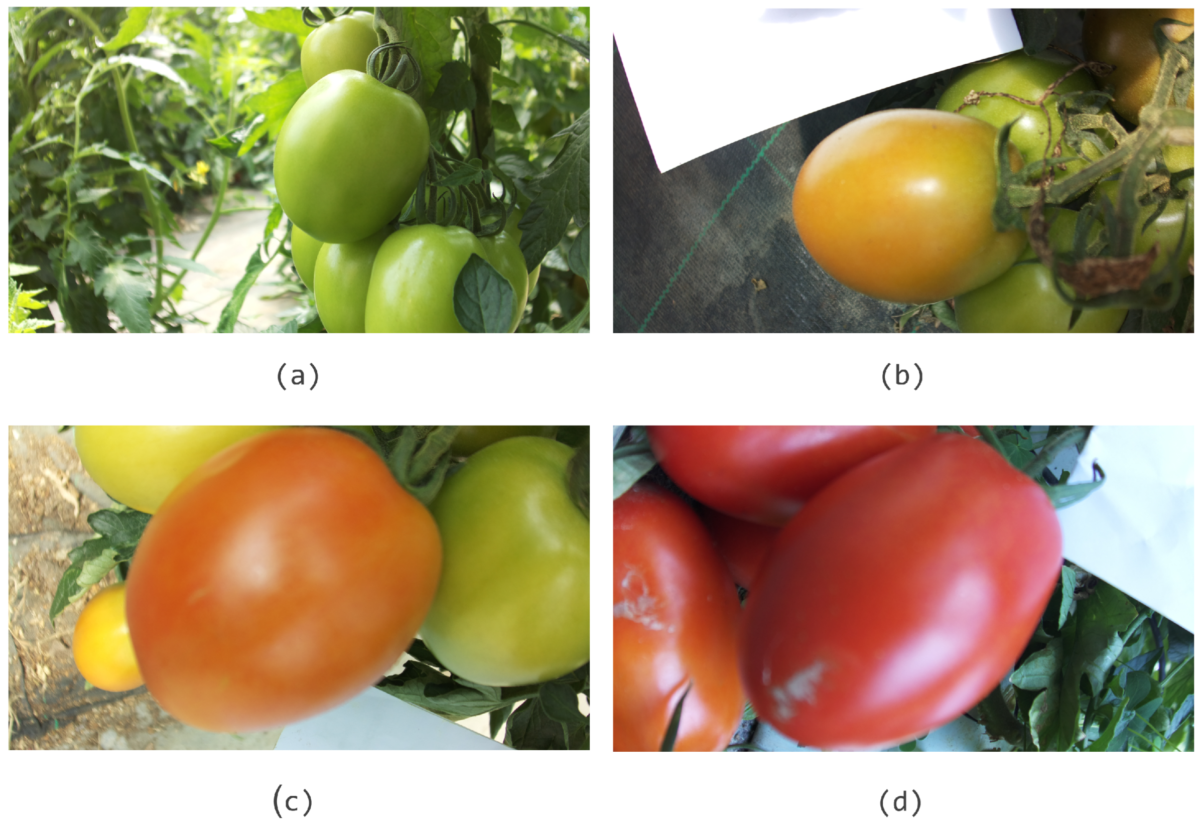
The general focus of the ML field is to predict an outcome using the available data. The prediction task can be called a “detection problem” when the outcome represents a single class. If the outcome represents different classes, it means a “classification problem” [63]. This study aims to detect and classify tomatoes using two one-stage object detection frameworks (SSD and YOLO). When it comes to classification, to differentiate the fruits according to their ripeness stage, four classes were defined based on the USDA colour chart for fresh tomatoes [64], as presented in Figure 2.

Figure 2. Classes defined according to the colour of tomato during ripening: Green (a)—more than 90% of the surface is green; Turning (b)—10 to 30% of the surface is yellow; Light Red (c)—between 60 to 90% of the surface is red; Red (d)—90 to 100% surface is red.

3.2. Deep Learning Approach

3.2.1. Dataset Structure

To train and evaluate the DL models, all images from the AgRobTomato Dataset and all images, except for the green tomato images, from the RpiTomato Dataset were selected. Since the AgRobTomato Dataset already had many green tomato images, it was decided not to select images of tomatoes at this stage of ripeness from the RpiTomato Dataset to balance the total set of selected images. A total of 632 images were selected.

Since it involves supervised learning, the models need to be provided with an annotated dataset. Thus, the images were manually annotated using the open-source annotation tool CVAT (see https://cvat.org/, accessed on 22 October 2021), indicating by rectangular bounding boxes the position and class of each plant. The images were annotated with the 4 chosen ripeness classes. After annotating, the images of both datasets were exported under the Pascal VOC format [65] and the YOLO format [66] to train the SSD and YOLO frameworks, respectively.

High-resolution DL models are time and computationally consuming and cannot process full-sized images, considering the input of square images, thus rescaling them before processing. For this reason, to avoid distortion, the original images of the AgRobTomato Dataset were split into images with a resolution of 720 × 720 px. Due to their original resolution, the RpiTomato Dataset images needed to be rescaled (961 × 720) px and cropped to achieve the 720 × 720 px resolution. The split operation doubled the images from the AgRobTomato Dataset, thus increasing the total number of images to 1081. However, some of them contained few annotations, and the splitting resulted in non-annotated images. These images were then removed from the dataset, being left with 1029 images.

To train and validate the different models, the images were divided into 3 sets:

• Training set—60% of the data;
• Validation set—20% of the data;
• Test set—20% of the data.

Data augmentation was used to artificially increase the dataset, improving the overall learning procedure and performance by inputting varied data into the model [67]. The transformations were carefully chosen, applying those that could happen in an actual robotic harvesting operation, just to the training and validation sets with a random factor, as displayed in Figure 3.

Figure 3. Different types of transformations applied to the images.

The data augmentation led to 7598 annotated images. The training and validation sets contained 5543 and 1850 images, respectively, while the test set was composed of 205 images.

3.2.2. Models Training

The literature refers to several ML frameworks, an interface, library, or tool that easily creates ML models [46]. In this study, the choice of framework falls on TensorFlow (see https://www.tensorflow.org/, accessed on 3 November 2021) [68], an open source easily scalable ML library developed by Google, which provides a collection of workflows to develop and train models using Python, C++, JavaScript, or Java.

TensorFLow r.1.15.0 was used for the training and inference scripts, which run on Google Collaboratory (Colab) notebooks (see https://colab.research.google.com/, accessed on 25 September 2021) that give free access to powerful GPU’s (Graphics Processing Unit) and TPU’s (Tensor Processing Unit) to develop DL models. Although the GPU’s available may vary for each Colab session, in general an NVIDIA Tesla T4 with a VRAM of 12 GB and a computation capability between 3.5 and 7.5 was assigned to all sessions. One pre-trained SSD MobileNet v2 model from the TensorFlow database (see https://github.com/tensorflow/models/blob/master/research/object_detection/g3doc/tf1_detection_zoo.md, accessed on 3 November 2021) and one YOLOv4 model from the Darknet database (see https://github.com/zauberzeug/darknet_alexeyAB, accessed on 3 November 2021) were considered in this study. Both models were pre-trained with Google’s COCO (Common Objects in Context) dataset (see https://cocodataset.org/#home, accessed on 3 November 2021) with an input size of 640 × 640 px (SSD MobileNet v2) and 416 × 416 px (YOLOv4).

Through transfer learning, a fine-tune was performed on pre-trained models to detect and classify tomatoes. Slight changes to the default training pipeline were made, such as adjusting the batch size for each model (24 to the SSD MobileNet v2 model and 64 to the YOLOv4 model) and removing data augmentation from the pipeline. The SSD MobileNetv2 model training sessions ran for 35,000 epochs, while the YOLOv4 model training was much faster, requiring only 8000 epochs. The number of epochs may vary from model to model, but in this case, was chosen based on the suggestion given by the literature, but mainly taking into account the “average loss” training metric, selecting the number of epochs that would be sufficient to converge. As far as the MobileNet v2 SSD model is concerned, an evaluation session occurred at every 50 epochs, following the standard value used by the pre-trained models. Since Darknet had no available validation sessions, it was not considered for the YOLOv4 model. These evaluation sessions are quite useful, since they allow monitoring the evolution of the training, meaning if the evaluation loss started to increase while the training loss decreased or remained constant, the deep learning model was over-fit to the training data.

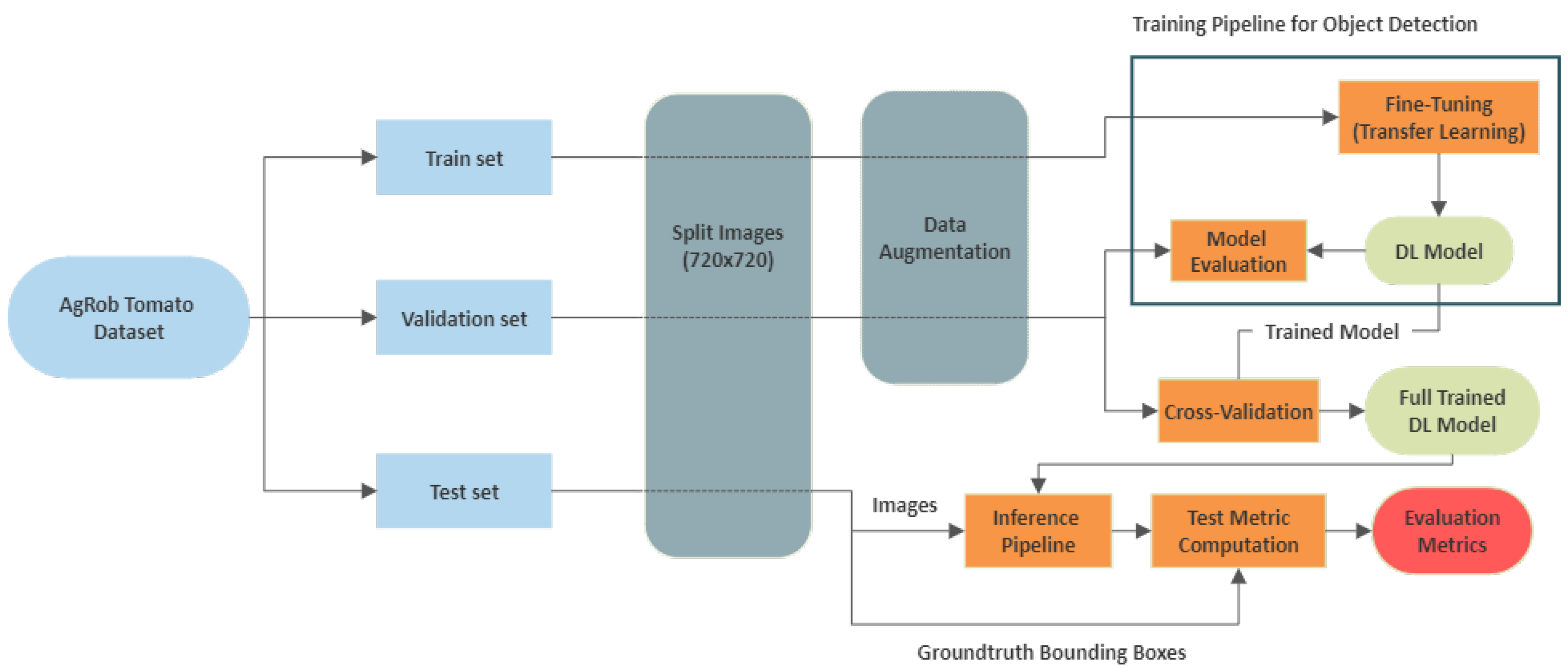
3.2.3. In a Nutshell

Figure 4 reports an overview of all the required steps used to reach the trained DL models.

Figure 4. Workflow of the performed methods to reach the trained DL models.

3.3. HSV Colour Space Model Approach

An approach based on histograms from the HSV colour space was developed as an alternative to DL models for tomato classification. All the scripts used throughout this process are authorship and were created from scratch through Spyder (see https://www.spyder-ide.org/, accessed on 25 October 2021). The developed HSV colour space model and the scripts can be found in the following GitHub repository: https://github.com/gerfsm/HSV_Colour_Space_Model (accessed on 25 October 2021).

In order to build the model, images of 10 tomatoes from each ripeness class were selected. To add some variability, half of the images come from the AgRobTomato Dataset and the other from the RpiTomato Dataset, as they present different perspectives of the fruits. The AgRobTomato Dataset offers a farther perspective, while in the RpiTomato Dataset the fruits are closer.

The first step was to extract the RoI from the images. All the images were labelled using the annotation tool CVAT and the coordinates of the annotation bounding box were used to segment the image and extract the RoI.

The next step was to convert the RoI images from RGB to HSV colour space. The RGB colour information is usually much noisier than the HSV information. Thus, using only the Hue channel makes a computer vision algorithm less sensitive, if not invariant, to problems like lighting variations. The image’s colour space conversion was performed through the function “cv.cvtColor()” (see https://docs.opencv.org/4.5.2/df/d9d/tutorial_py_colorspaces.html, accessed on 13 June 2021) from OpenCV [69].

For each HSV image, a colour histogram was generated focusing only on the Hue channel. OpenCV was used to extract the colourimetric data from the RoI. Different applications use different scales to represent the HSV colour space. For the Hue values, OpenCV uses a scale ranging between 0 and 179. Since the interest is focused on analysing the region of colours that a tomato can display, the entire colour spectrum is unnecessary. Therefore, the location of the origin for the Hue parameter was changed, giving the histogram a seemingly normal distribution. Through Matplotlib [70], the function “matplotlib.pyplot.hist” (see https://matplotlib.org/stable/api/_as_gen/matplotlib.pyplot.hist.html, accessed on 22 July 2021) was used to plot the H-spectrum histogram. In this case, the function parameter “density” was set to “True”, which causes a probability density to be drawn and returned. It was preferred to use all the bins in the range to get as accurate a model as possible. Each bin displays the bin’s raw count divided by the total number of counts and the bin width so that the area under the histogram integrates to 1.

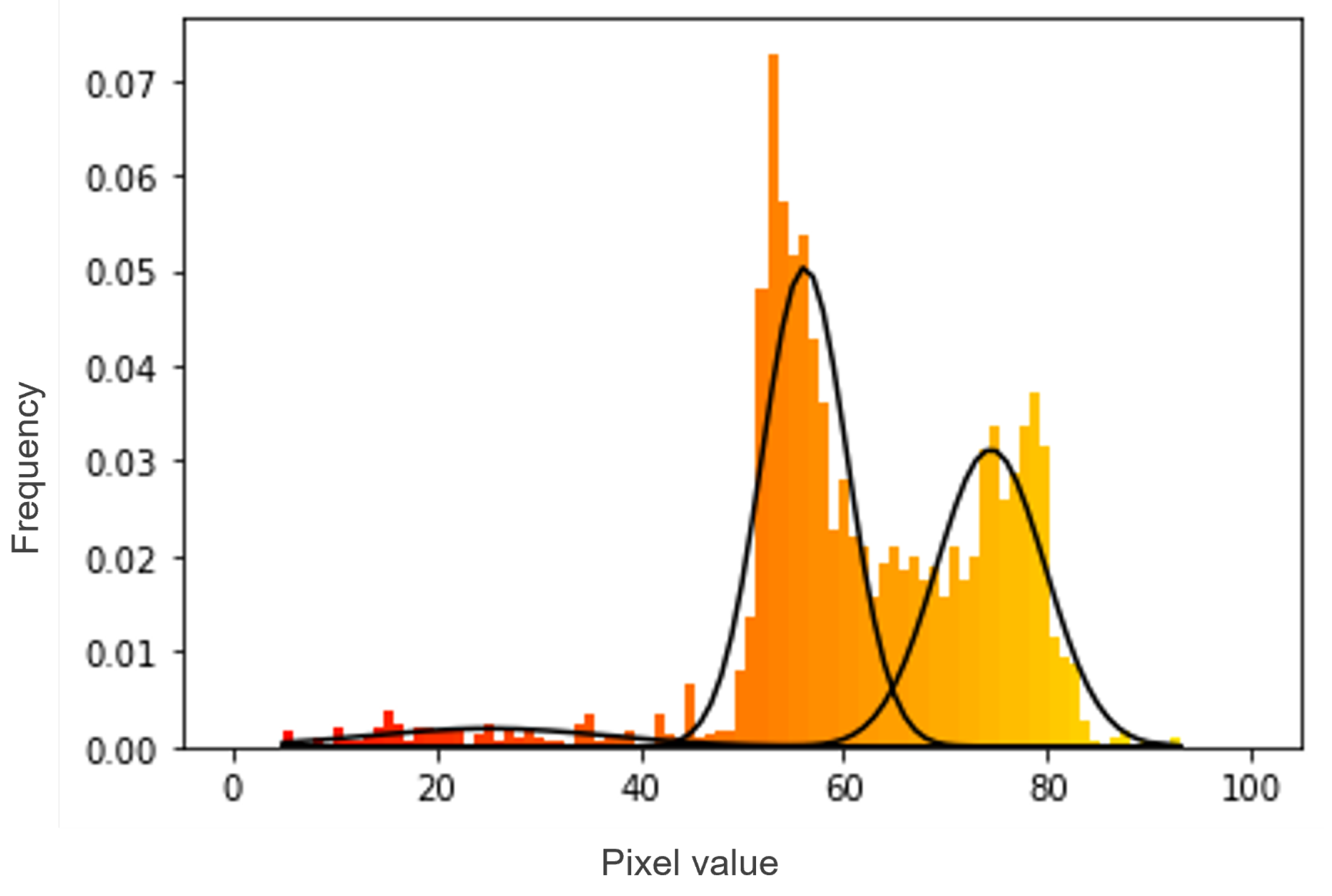
Although the segmentation technique used is faster and easier to implement, it can be noted that the RoI covers the object to be classified and some of the background, which slightly affects the results obtained. In some cases, the background makes the data look multimodal, i.e., there is more than one “peak” data distribution. Trying to fit a multimodal distribution with a unimodal (one “peak”) model will generally give a poor fit and lead to incorrect classifications.

Gaussian mixture model was used to overcome this problem. This function is a probabilistic model for representing normally distributed subpopulations within an overall population (Figure 5) and was applied using the “sklearn.mixture.GaussianMixture” (see https://scikit-learn.org/stable/modules/mixture.html, accessed on 29 July 2021) function, from Sklearn (or scikit-learn) [71].

Figure 5. Representation of the H-spectrum and a Gaussian mixture model probability distribution.

3.3.1. Gaussian Filtering Approach

The next step was to choose the Gaussian with the highest peak, which corresponds to the RoI and ignore the rest. The curve was selected according to the Gaussian mixture weights. These weights are normalised to 1, motivated by the assumption that the model must explain all the data, then use the law of total probability. So, in that sense, they are the probabilities of the point being part of the cluster. In other words, the weights are the estimated probability of a draw (i.e., distribution curve) belonging to each respective normal distribution. Even with the background noise, the data distribution in the RoI zone is well defined. The probability that this region is a normal distribution is much higher, meaning that the weight is higher. Selecting the higher weights leads to the RoI Gaussian, thereby enabling to separate pixels of tomatoes from pixels of the background. For a more careful analysis, a boxplot was also generated for each RoI, through the function “matplotlib.pyplot.boxplot” (see https://matplotlib.org/stable/api/_as_gen/matplotlib.pyplot.boxplot.html, accessed on 29 July 2021). The boxplots represent the values within 3 standard deviations of the mean, corresponding to 99.7% of the Gaussian.

Based on the results obtained, correlating the Hue histogram mean of each sample with its respective class, a statistical classifier was reached. These results will be presented and exploited later in the respective Section 4.1.

3.3.2. In a Nutshell

Figure 6 reports an overview of all the required steps used to reach the proposed HSV colour space model.

Figure 6. Workflow of the performed methods to reach the HSV colour space model.

3.4. Evaluation Metrics

Although the DL models were trained with four classes, besides the classification problem, they were also evaluated for their ability to detect, i.e., locate the fruits in the image regardless of their ripeness stage. The HSV colour space model was only evaluated for the classification problem.

A “correct detection” is commonly established through the Intersection over Union (IoU) metric, measuring the overlapping area between the predicted bounding box (B_p) and the groundtruth bounding box (B_gt) divided by the union area (1). In this case, a correct detection was considered if IoU >= 50%.

$$\mathrm{IoU}=\frac{\mathrm{Area}(B_{\mathrm{p}}\cap B_{\mathrm{g}\mathrm{t}})}{\mathrm{Area}(B_{\mathrm{p}}\cup B_{\mathrm{g}\mathrm{t}})}$$

(1)

To better benchmark the two DL models, the metrics used by the Pascal VOC challenge [65] (Precision × Recall curve and Mean Average Precision) were chosen, with the addition of the following metrics:

• Recall (2)—ability of the model to detect all the relevant objects (i.e., all groundtruth bounding boxes);
• Precision (3)—ability to identify only the relevant objects;
• F1-Score (4)—first harmonic mean between Recall and Precision.

The number of groundtruths (relevant objects) can be computed by the sum of the True Positives and False Negatives (TP + FN) and the number of detections is the sum of the TP’s and False Positives (TP + FP). TP’s are the correct detections of the groundtruths, FP’s are improperly detected objects and FN are undetected.

$$\mathrm{Recall}=\frac{\mathrm{TP}}{\mathrm{TP}+\mathrm{FN}}=\frac{\mathrm{TP}}{\mathrm{All}\mathrm{groundtruths}}$$

(2)

$$\mathrm{Precision}=\frac{\mathrm{TP}}{\mathrm{TP}+\mathrm{FP}}=\frac{\mathrm{TP}}{\mathrm{All}\mathrm{detections}}$$

(3)

$$\mathrm{F}1-\mathrm{Score}=2\times \frac{\mathrm{Precision}\times \mathrm{Recall}}{\mathrm{Precision}+\mathrm{Recall}}$$

(4)

All the detections performed by a DL model have a confidence rate associated with them. Graphically representing the ratio between Precision and Recall (Precision × Recall curve) can be seen as a trade-off between Precision and Recall for different confidence values associated with the bounding boxes generated by a detector. A great object detector keeps its Precision rates high, while its Recall increase. Thus, a high Area Under the Curve (AUC) tends to indicate both high Precision and Recall.

However, it is difficult to accurately measure the AUC, as the Precision × Recall curve is often a zigzag-like curve. To overcome this problem was calculated the Average Precision (AP) metric by the all-point interpolation approach. In this case, the AP (5) is obtained by interpolating the Precision at each level, taking the maximum Precision (P_interp(R)) call value is greater or equal than R_n+1.

$$\mathrm{AP}=\sum _{\mathrm{n}}(R_{\mathrm{n}+1}-R_{\mathrm{n}})P_{interp}\left(R_{\mathrm{n}+1}\right)$$

(5)

If there is more than one class to detect, the Mean Average Precision (mAP) metric is used, simply the average AP over all classes (6). AP_i represents the AP of class i and NC is the number of classes evaluated.

$$\mathrm{mAP}=\frac{{\sum }_{\mathrm{i}=1}^{\mathrm{NC}}{\mathrm{AP}}_{\mathrm{i}}}{\mathrm{NC}}$$

(6)

The final step of the inference was to optimise the confidence score, using the cross-validation technique: validation set augmentations were removed, and the F1-Score was computed for all the confidence thresholds from 0% to 100%, into steps of 1%. The confidence threshold that optimises the F1-Score was selected for the model’s normal operation. The test set was used to evaluate both models, and the whole inference process occurred on the Google Colab server, using a Tesla T4 GPU.

To assess the classification ability, the evaluation metrics chosen were the Precision and Recall for each class that will act as building blocks for the Macro F1-Score and Balanced Accuracy metrics. The Balanced Accuracy metric is a simple arithmetic mean of Recall of each class (7). To achieve the Macro F1-Score, it is necessary to compute Macro-Precision and Macro-Recall, computed as the arithmetic means of the metrics for single classes (8). These metrics give each class the same weight in the average, so that there is no distinction between highly and poorly populated classes, which is useful in cases of unbalanced datasets.

$$\mathrm{Balanced}\mathrm{Accuracy}=\frac{{\sum }_1^{\mathrm{No}.\mathrm{Classes}}\frac{\mathrm{TP}}{\mathrm{Total}\mathrm{Groundtruths}}}{\mathrm{No}.\mathrm{Classes}}$$

(7)

$$\mathrm{Macro}\mathrm{F}1-\mathrm{Score}=2\times \frac{\mathrm{Macro}\mathrm{Precision}\times \mathrm{Macro}\mathrm{Recall}}{\mathrm{Macro}\mathrm{Precision}+\mathrm{Macro}\mathrm{Recall}}$$

(8)

4. Results

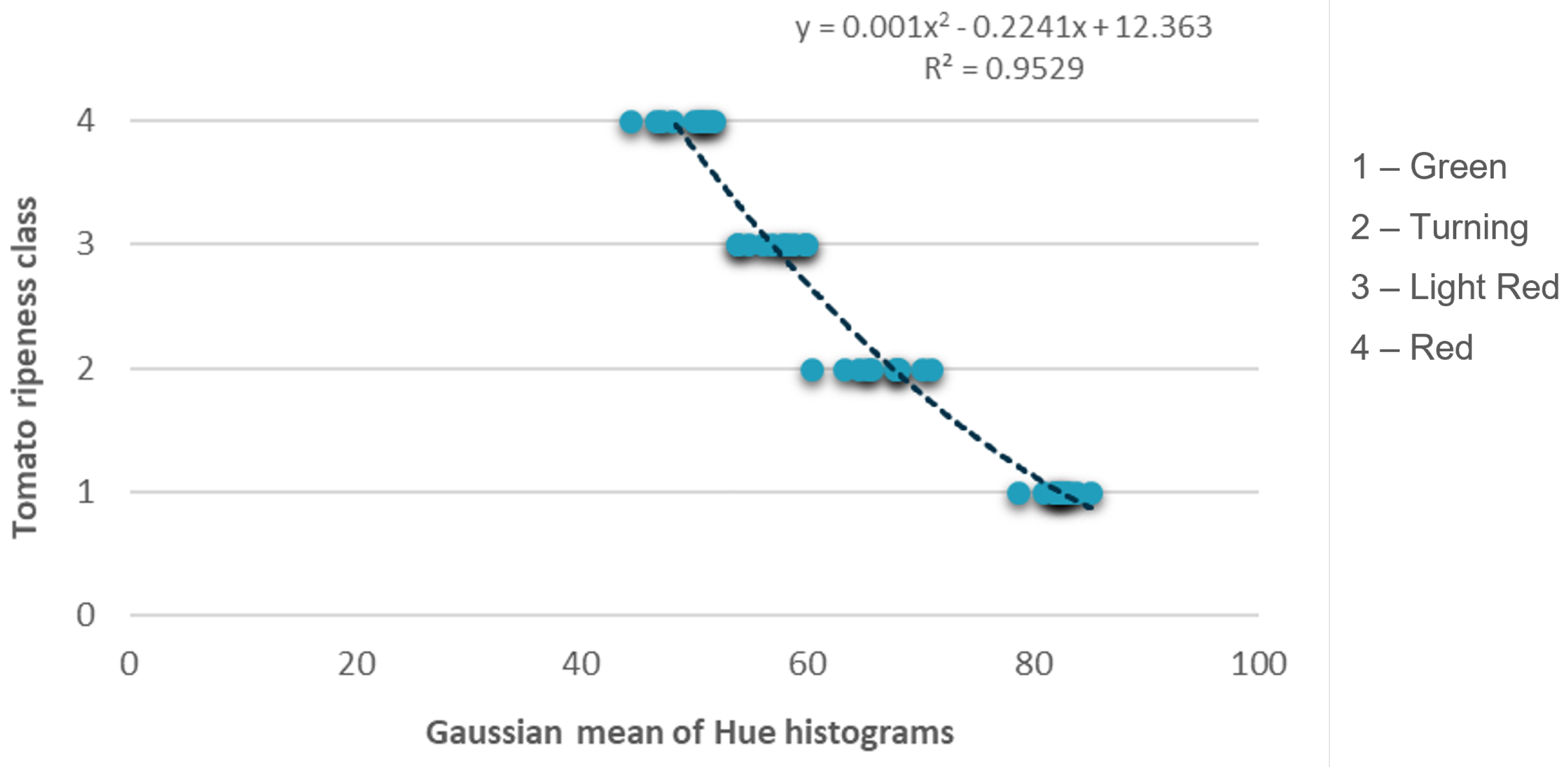
4.1. HSV Colour Space Model Classifier

Based on the Hue histogram mean of each sample used to build the model and its correlation with the respective class, a quadratic function was obtained as the statistical classifier through the Microsoft Excel tool (Figure 7).

Figure 7. Correlation between the Hue histogram Gaussian mean of each sample with its respective class, along with the plot of the tendency line, equation and R² of the quadratic function obtain.

To classify the tomatoes, it was necessary to define the thresholds for each class. By fine-tuning the equation, namely adding 0.25 to the independent term, the following was established (9):

$$f\left(x\right)=\left\{\begin{array}{cc}Green,\hfill & if 000.1x^2-0.2241x+12.613\le 1.5\hfill \\ Turning,\hfill & if 1.5<000.1x^2-0.2241x+12.613\le 2.5\hfill \\ LightRed,\hfill & if 2.5<000.1x^2-0.2241x+12.613\le 3.5\hfill \\ Red,\hfill & if 000.1x^2-0.2241x+12.613>3.5\hfill \end{array}\right.$$

(9)

Achieving the classifier culminated in the ultimate model. For a specific image, given the bounding boxes coordinates of the fruits to be classified (input), in a single pass, the HSV colour space model segments the RoI’s, converts them to the HSV colour space, through the colourimetric information. Furthermore, the Gaussian Mixture probabilistic model generates a histogram and calculates its mean that through the statistical classifier generates an output. The model returns the class to which that fruit belongs.

4.2. Tomato Detection Using Deep Learning Models

As mentioned, the models required defining the best confidence threshold before evaluating their performance. Table 3 indicates the value of the confidence threshold that maximises the F1-Score for each model, finding the best balance between the Precision and Recall, optimising the number of TP’s while avoiding the FP’s and FN’s. Both models found their best F1-Score at similar confidence thresholds, i.e., similar confidence in their predictions. However, the YOLOv4 model achieved a better F1-Score of 86%.

Table 3. Confidence threshold for each DL model that optimises the F1-Score metric.

DL Models	Conf. Threshold ≥	F1-Score
SSD MobileNet v2	56%	74.16%
YOLOv4	58%	86.01%

Figure 8 reports the evolution of the F1-Score with the variation of the confidence threshold for cross-validation. It is possible to infer that the models behave slightly different. Models with flattened curves indicate higher confidence in their predictions and a low amount of FPs and FNs. Such is the case with the SSD MobileNet v2 model. Despite having a lower F1-Score, it is more consistent, as it can maintain essentially the same F1-Score value over the confidence threshold.

Figure 8. Evolution of the F1-score with the variation of the confidence threshold for both DL models in the validation set without augmentation.

The previous analysis provided the benchmark in the validation set. The results presented below refer to the benchmarking of the test set that allows understanding the generalisation capacity of the trained DL models.

Table 4 shows the results across the different metrics, considering all the predictions and the best-computed confidence threshold. Lower confidence rates tend to have lower Precision but a higher Recall rate. Hence, limiting the confidence threshold can become an advantage, as can be seen by the YOLOv4 model results. When the model has full freedom to make predictions (confidence threshold ≥ 0), it presents a Recall up to 96%, but a Precision only around 16%, drastically affecting the F1-Score. However, by limiting the confidence threshold, the model could obtain a higher Precision without harming the Recall rate too much (still above 84%), thus obtaining an excellent F1-Score.

Table 4. Detection results of the DL models over the evaluation metrics, considering all the predictions and the best computed confidence threshold.

DL Models	Conf. Threshold ≥	Inference Time	mAP	Precision	Recall	F1-Score
SSD MobileNet v2	0%	0.067 s	67.82%	74.76%	73.72%	74.03%
YOLOv4	0%	0.073 s	90.02%	16.45%	95.84%	28.07%
SSD MobileNet v2	56%	0.067 s	65.38%	77.62%	70.12%	73.68%
YOLOv4	58%	0.073 s	82.97%	86.73%	84.90%	85.81%

Another important aspect is the inference time, quite similar in both models, with a slight advantage for the SSD MobileNet v2 model (0.067 s), reaching good and expected values considering that we are talking about one-stage detectors.

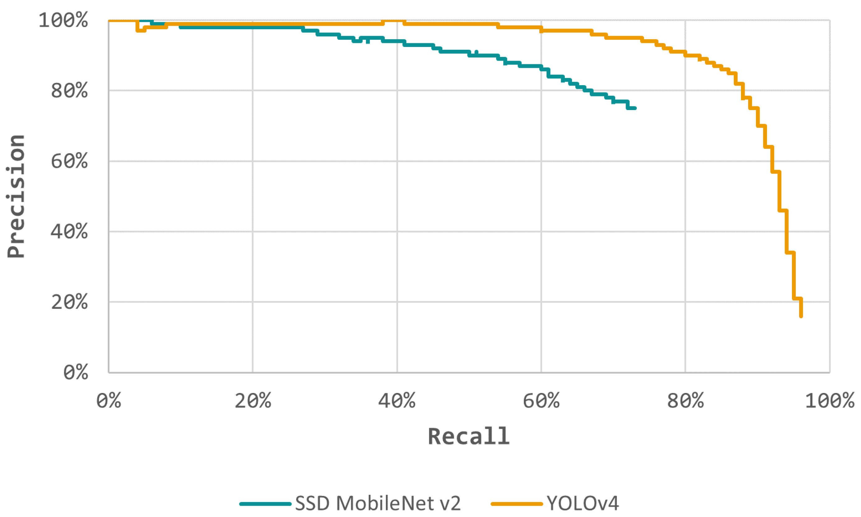
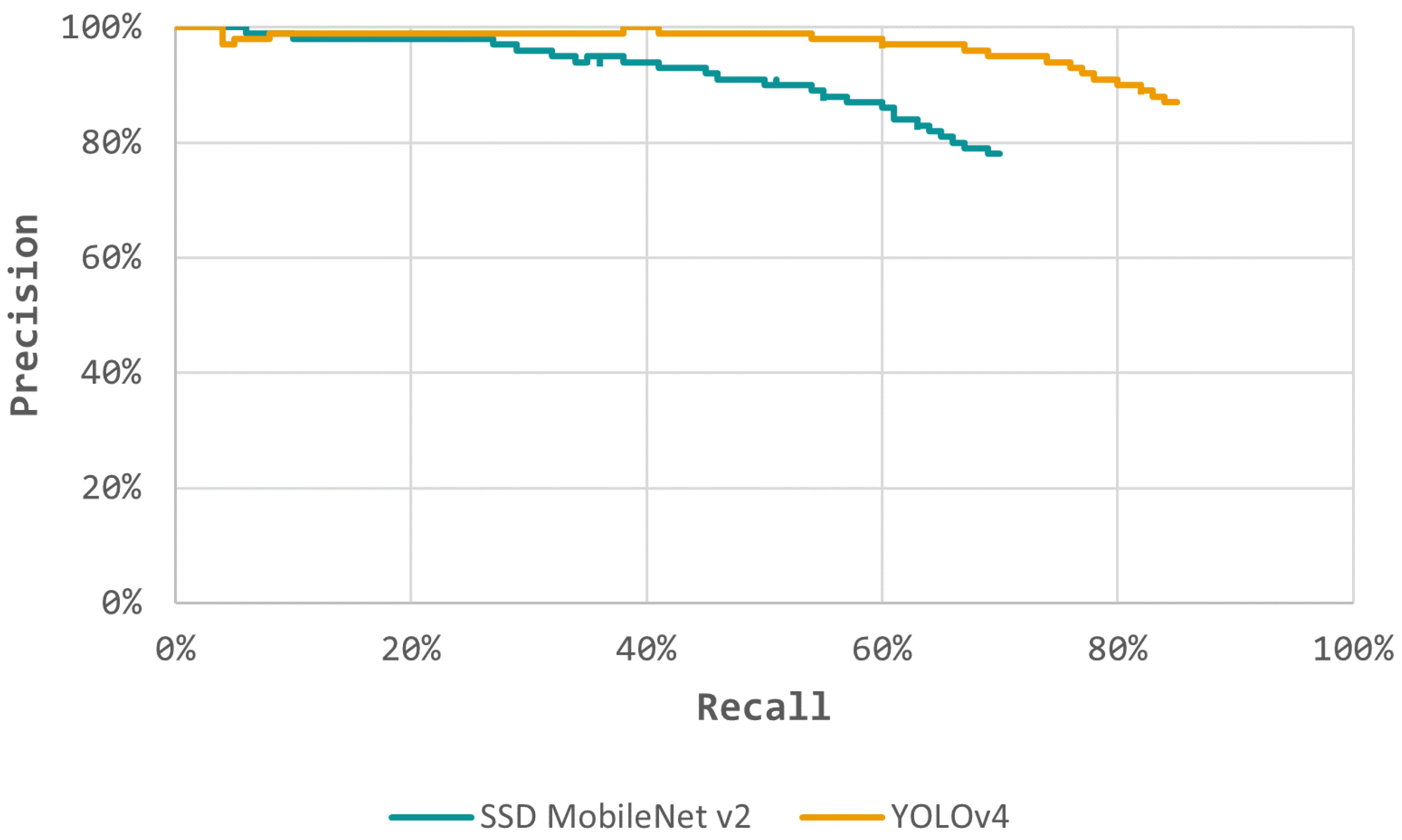
Figure 9 shows a Precision x Recall curve built using all the predictions. The best performing model has the highest AUC, therefore the YOLOv4 model. However, the low Precision at higher Recall rates and the lower F1-Score indicates that the model has much prediction noise and false positives. Thus, considering all the model predictions, using the F1-score as a balanced metric between the Recall and Precision, SSD MobileNet v2 was the best performing model, with an F1-Score of 74.03%.

Figure 9. Precision × Recall curve for both DL models considering all the predictions.

Performing an additional filtering process on the predictions, the Recall × Precision curve was now transformed through a truncation process (Figure 10). Both models had a Precision rate higher than 75%, with the YOLOv4 model almost achieving 87%. Recall and Precision rates were similar for both models, especially on the YOLOv4 model, which shows that the models are well balanced. Furthermore, the models had a high confidence rate in their predictions, with the YOLOv4 model standing out, reaching an F1-Score close to 86%, meaning that it possesses the ability to detect almost all groundtruths, without neglecting Precision, i.e., having few FP’s.

Figure 10. Precision × Recall curve for both DL models using the best confidence threshold.

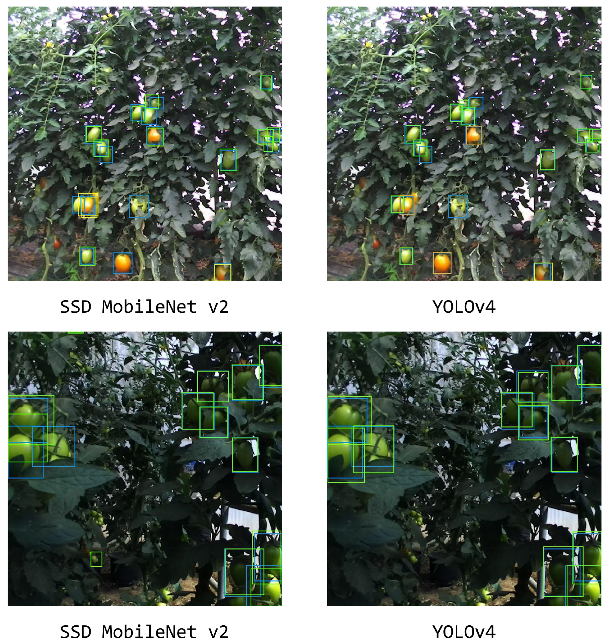
Figure 11 allows to perceive, from image analysis, the capacity of the DL models through representative images of the test set. Both models had a good response in tomato detection, dealing very well with the complexities of the environment. The models were able to detect green tomatoes with high colour correlation with the background. Furthermore, in poor lighting situations, both models performed well, showing robustness and capability to deal successfully with problems posed by different lighting conditions. In cases where tomatoes are occluded by branches, stems, leaves or other tomatoes (overlapped), the models showed a great performance.

Figure 11. Detection results comparison between the two DL models in situations of lesser or greater complexity. Blue bounding boxes represents groundtruth annotations; Green, Yellow, Orange and Red bounding boxes represents Green, Turning, Light Red and Red tomatoes predictions, respectively.

4.3. Tomato Ripeness Classification: Deep Learning vs. HSV Colour Space Models

Regarding the classification problem, Table 5 presents the results for the different metrics used in the evaluation of the two DL models and the proposed HSV colour space model. All models were able to distinguish the Red tomato class very well, with Precision rates above 80%, with the HSV colour space and the YOLOv4 models standing out with around 89%. However, they still had much more struggle to classify all relevant objects of this class, unlike the SSD MobileNet v2 model, which achieved a Recall of 84%.

Table 5. Classification results of the over the evaluation metrics, considering each model’s best-computed confidence threshold.

DL Models	Fruit Ripeness	Precision	Recall	Macro F1-Score	Balanced Accuracy
SSD MobileNet v2	Green	77.27%	70.09%	65.93%	62.70%
	Turning	59.38%	55.88%
	Light Red	60.61%	40.82%
	Red	80.77%	84.00%
YOLOv4	Green	85.38%	84.66%	74.16%	68.87%
	Turning	70.77%	67.65%
	Light Red	76.32%	59.18%
	Red	88.89%	64.00%
HSV Colour Space	Green	98.24%	98.31%	70.93%	68.10%
	Turning	50.00%	63.24%
	Light Red	58.33%	42.86%
	Red	89.47%	68.00%

On the other hand, the complexity of detecting and subsequently classifying green tomatoes affected the SSD MobileNet v2 model much more. The YOLOv4 and HSV colour space models obtained excellent results, both in Precision and Recall, with the proposed model standing out with rates higher than 98% in both metrics.

It is noticeable that there was considerable difficulty in distinguishing Turning and Light Red class tomatoes by all models, especially the MobileNet v2 SSD and HSV colour space which could not detect even half of the relevant objects of the two classes, with poor Recall rates of around 43%.

Macro F1-Score and Balanced Accuracy metrics provides a general and better understanding of the results obtained. YOLOv4 model outperformed the SSD MobileNet v2 and HSV colour space models with a Macro F1-Score of 74.16%. The low value obtained by the SSD MobileNet v2 model was highly affected by its weak ability to distinguish between Turning and Light Red tomatoes.

Regarding the Balanced Accuracy, the YOLOv4 model was again better at classifying the fruits, with 68.87% of Balanced Accuracy. However, the HSV colour space model achieved a very similar result (68.10%) mainly due to its strong ability to classify Green and Red class tomatoes.

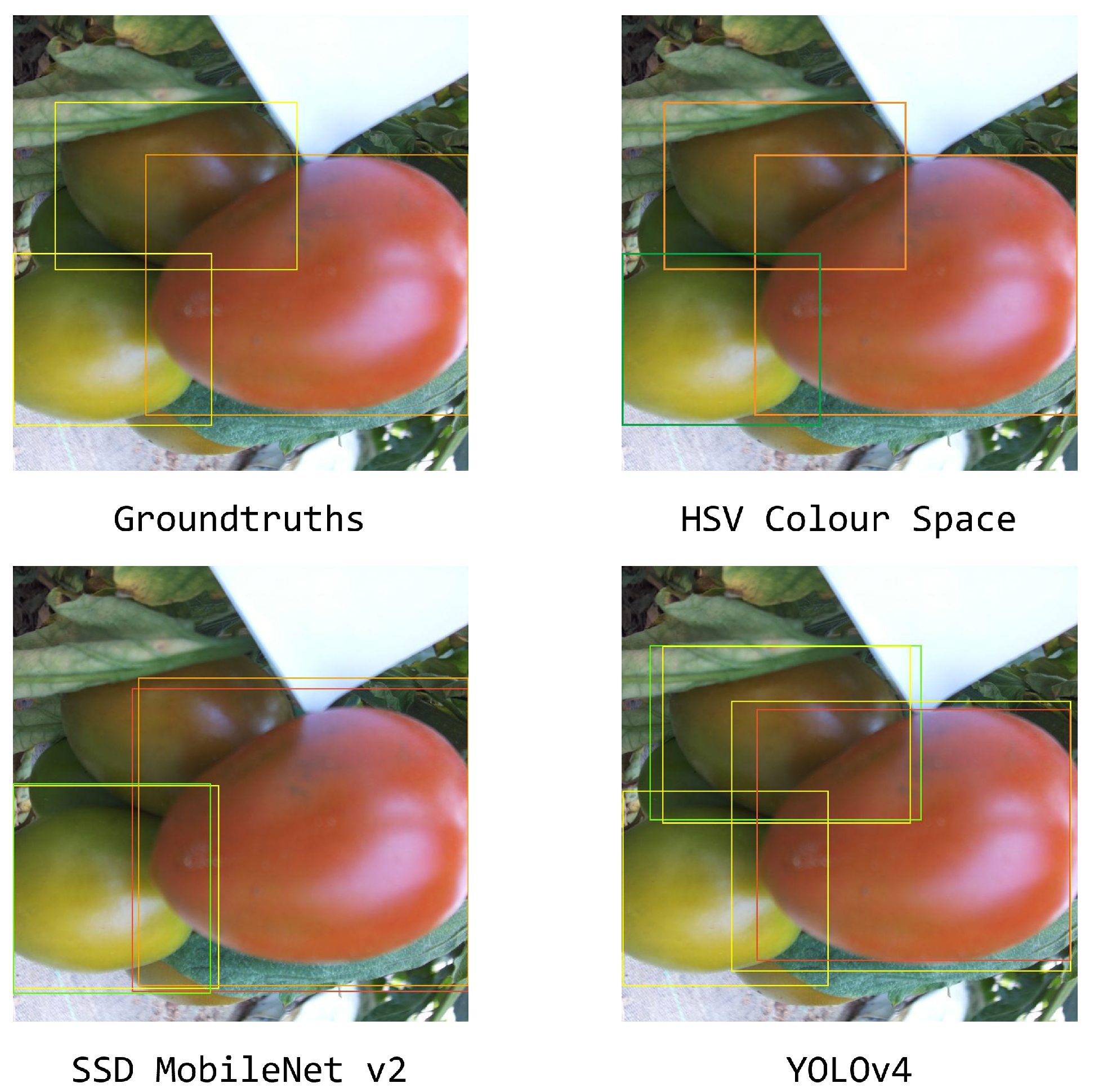
Figure 12 illustrates cases of poor classifications due to the difficulty of the models in distinguishing some tomato classes. An interesting aspect is how the DL models dealt with these situations. For some fruits, the models drew two bounding boxes of different classes. The tomatoes are correctly detected, but at least one of the class predictions is incorrect, which ultimately affects the classification results obtained.

Figure 12. Classification results comparison between the two DL models and the HSV colour space model with the groundtruth annotations. Green, Yellow, Orange and Red bounding boxes represents Green, Turning, Light Red and Red tomatoes predictions, respectively.

5. Discussion

This work proposed the training and testing of two DL models for tomato detection and compared them with a developed HSV colour space model regarding the classification of those fruits according to their colour/ripeness through images of two datasets collected for this effect.

Overall, both models were generic enough to detect tomato successfully. The results were similar between the validation set and the test set, with the YOLOv4 model obtaining promising results, being the best performing model. Interestingly, the use of filtered results by a threshold was only significant to the YOLOv4 model. The SSD MobileNet v2 model obtained identical results regardless of the confidence threshold, which means that it can be used without any filtering process without compromising the results. The models were able to detect tomatoes at different ripeness stages, even in complex scenarios, considering occlusions, overlaps and variations in illumination conditions. As they are one-stage detectors, the SSD MobileNetv2 and YOLOv4 models, although faster at detecting, could lack accuracy. This is not overly verified, showing good inference times that, together with the results of Precision and Recall, allow these models to be applied in systems equipped with computer vision to perform tasks in real time.

Comparing these results with different authors is essential to understand the relevance of the results obtained and potential aspects that could be improved. Both models outperformed with distinction those presented by Yuan et al. [28], Magalhães et al. [49], Padilha et al. [50] and Rupareliya et al. [55], which obtained quite high Precision rates but ended up failing in their ability to detect all relevant objects, causing the overall F1-Score to vary only between 60 and 66%. The models evaluated in this paper only lagged behind some heavily modified models. Chen et al. [51], Liu et al. [53], Lawal [56] and Xu et al. [54] improved the YOLOv3 and YOLOv3 Tiny models leading to an F1-Score consistently higher than 90%. However, most of these models were trained with a single class, regardless of the fruit ripeness stage, and in some cases the datasets were largely or entirely composed of red tomatoes which, due to the higher colour contrast between the fruit and the background, are easier to detect. To the best of our knowledge, there is no literature reporting the application of DL models in the detection of tomato in a greenhouse context with more than three classes. Therefore, taking into account that the models were lightly modified and trained with four classes with real greenhouse environment images, the SSD MobileNet v2 and YOLOv4 model results are very promising, even more so considering that the latter achieved an F1-Score close to 86%.

When it comes to classification ability, the DL models behaved quite differently. The results did not follow the detection ones, largely due to the difficulty of the models in distinguishing the intermediate classes (Turning and Light Red). The similarity in terms of colour between the two classes may interfere with the results. Besides, even to the human eye, the distinction of the fruits between these classes can be somewhat subjective and imprecise. This is reflected in the annotation process itself that, at the training level, can make complex the models learning. Nevertheless, both models achieved great results in the Green and Red class tomatoes classification.

As an alternative in classification, an HSV colour space model was proposed. The model obtained superb results in the Green class tomatoes classification but struggled to distinguish tomatoes from the Turning class with the Light Red class. A possible reason for this is the Gaussian mixture model used. It is an iterative algorithm that is not optimal. As such, especially in frontier classes, it does not always give the same result that varies according to what was initially assumed. Still, it outperformed the SSD MobileNet v2 model with distinction and came close to the YOLOv4 model, especially regarding the Balanced Accuracy. The results become more interesting when one realises that to achieve these results, the DL models had to be trained with a large number of images (7393 images). In contrast, the HSV colour space model was developed with only 40 images (10 from each class). Another advantage of the proposed model is its simplicity, making it more intuitive and accepted: adjusting the number of classes required and changing the confidence thresholds for each class.

The sorting of fruits based on their ripeness stage is an operation much more associated with post-harvest. For this reason, in the overwhelming majority of studies, the classification of fruits is done in a structured environment. This is similar to that found in processing industries after the fruits are harvested. The only relevant paper that has evaluated the ability of DL models to classify tomatoes is from Mutha et al. [58], who achieved an average accuracy of 94.67% through a YOLO architecture in the classification of 3 distinct tomato classes. Despite this, the tomato images used do not even represent the agricultural environment in general, nor a greenhouse, in particular, and the test set only contained 23 images. Regarding more conventional methods, through colour-based models, Benavides et al. [34] achieved an accuracy of 77% through the aggregated percent surface area below certain Hue angles, when classifying tomatoes in 6 different ripening stages. Using the HSV colour space to classify tomatoes into 5 classes, Gupta et al. [44] proposed a colour histogram matching and Malik et al. [35] used a K-Nearest Neighbour obtaining an accuracy of 97.20% and 100%, respectively. Although these studies show better results than our proposed HSV colour space model, they were all conducted with images of tomatoes detached from the plant, in an artificial environment, with a stable and solid background. All this demonstrates and makes our work groundbreaking since it was carried out with images of a real greenhouse environment, aimed at evaluating not only the detection but also the classification of tomatoes at different ripeness stages.

In summary, the DL models performed well in the detection task but had more difficulty in the classification one, with the HSV colour space model outperforming the SSD MobileNet v2 model. The different models have their advantages and disadvantages. The DL models are more time and computationally demanding. However, unlike the HSV colour space model, they handle complex scenarios a lot better, which can have a big influence on the performance of more elementary methods. Getting the best out of each model, an alternative could be modifying and fusing a DL model with the proposed HSV colour space model, to create a framework capable of detecting a greater number of fruits and classify them correctly without much loss in both moments. Some work has been developed along this line of thought, such as the one carried out by Ko et al. [72] that proposes a novel method for classifying tomato ripeness by utilizing multiple streams of CNN and their stochastic decision fusion, however, once again, the study was conducted in an artificial environment, still lacking the transfer and applicability of these models in a real agricultural context. Our publicly available datasets also contributes to scientific progress with the potential to be used to train and develop more accurate visual perception solutions for operation in a greenhouse context.

6. Conclusions

In this paper, two pre-trained DL models were benchmarked in tomato detection and compared with a HSV colour space model in the classification of those fruits in four maturity classes. Two datasets of tomato images in greenhouses were acquired for that purpose.

The YOLOv4 model best detected tomatoes, achieving an F1-Score of 85.81%, with a good tradeoff between the Precision and Recall rates. The results of the classification task were satisfactory and promising, with the YOLOv4 model standing out once again with a Macro F1-Score of 74.16%. The HSV colour space model outperformed the SSD MobileNet v2, obtaining a Balanced Accuracy similar to the YOLOv4 model of 68.10%. All models had more difficulty classifying tomatoes of the intermediate classes (Turning and Light Red). Although less demanding in its development, the HSV colour space model does not deal as well as DL models with highly complex scenarios.

In perspective, putative future work should go through: (i) enlarge the dataset, balancing it with more images with Red tomatoes; (ii) evaluating the performance of these models in on-time conditions, inside the greenhouses; (iii) benchmark this DL models against new and more optimized backbone networks, such as ResNet18, ResNet50, SE-ResNet, SENet-154 [73] or ViT vision transformers [74] and (iv) improve the HSV colour space model to better deal with the problems of the complex environment, considering an image segmentation DL model or develop an algorithm for tomato boundaries detection inside the bounding box, by formalizing a thresholding algorithm that picks the most reddish pixel and analyzes all neighbors without a drastic change to green (background).