Evaluation and Development of Pedo-Transfer Functions for Predicting Soil Saturated Hydraulic Conductivity in the Alpine Frigid Hilly Region of Qinghai Province

Abstract

In recent years, Pedo-Transfer Functions (PTFs) have become a commonly used tool to predict the hydraulic properties of soil. As an important index to evaluate the function of forest water conservation, the prediction of saturated hydraulic conductivity (K_S) on the regional scale is of great significance to guide the vegetation construction of returning farmland to forest area. However, if the published PTFs are directly applied to areas where the soil conditions are different from those where the PTFs are established, their predictive performance will be greatly reduced. In this study, 10 basic soil properties were measured as input variables for PTFs to predict K_S in the three watersheds of Taergou, Anmentan, and Yangjiazhai in the alpine frigid hilly region of Qinghai Province, China. The parameters of the eight published PTFs were modified by the least-squares method and new PTFs were also constructed, and their prediction performance was evaluated. The results showed that the K_S of coniferous and broad-leaved mixed forests and broad-leaved pure forests in the study area were significantly higher than those of pure coniferous forests, and grassland and farmland were the lowest (p > 0.05). Soil Organic Matter plays an important role in predicting K_S and should be used as an input variable when establishing PTFs. The Analysis-Back Propagation Artificial Neural Network (BP ANN) PTF that was established, with input variables that were, Si·SOM, BD·Si, ln²Cl, SOM², and SOM·lnCl had a better predictive performance than published PTFs and MLR PTFs.

1. Introduction

Soil, as an important link in the Soil-Plant-Atmosphere Continuum (SPAC) system, exerts an important influence on global terrestrial surface water and energy balance by regulating local water balance through infiltration, runoff, and groundwater recharge [1]. Saturated hydraulic conductivity (K_S), an important physical characteristic of soil, refers to the water flux or seepage velocity per unit area when the water potential gradient is fixed and the soil reaches saturation state [2]. To some extent, K_S can be used as an index to evaluate the ability of soil to conserve water and resist erosion. Although some studies have shown that the soil preferential flow plays a dominant role in groundwater recharge and chemical transport [3,4,5], the flowability of saturated flow in soil has a significant influence on the generation and development of surface runoff. Hence, K_S plays an important role in solving the management problems of soil and water resources related to agricultural production and ecological environment [6]. Meanwhile, K_S is usually a sensitive input variable in many hydrological models such as HYDRUS, TOPMODEL, and DHSVM, so whether K_S is accurate or not will directly affect the simulation results of the models [7]. K_S is not only an important variable in the Darcy equation to calculate the velocity in saturated soil, but is also crucial in unsaturated flow equations such as the Richards equation.

As for the determination of K_S, representative soil samples are usually collected in the study area and brought back to the laboratory for measurement. Common indoor measurement techniques are the Guelph permeameter in situ method and the constant head permeameter laboratory method [8,9]. Furthermore, there are some methods of field measurement. Although laboratory or field measurements are well developed, it is not easy to measure K_S over a large study area. Due to the strong spatial variability of K_S, more representative soil samples are needed to characterize the soil hydraulic characteristics in the study area, which will take a considerable amount of time and cost to carry out the large-scale application and be unrealistic if the study area is large [10,11]. To solve this problem, some scholars have developed Pedo-Transfer Functions (PTFs) to estimate the hydraulic properties of soils. PTFs refer to a function established by linking the hydraulic properties of soil with other soil properties (such as mechanical composition, bulk density, organic matter content, etc.) that are more easily obtained [12]. Over the past few decades, many PTFs from theoretical research to small-scale, to regional and global scales have been developed by soil scientists for a variety of purposes [11]. Wosten et al. have provided a comprehensive overview of the research that has been carried out in this research field [7]. Most of the original PTFs were built based on regression methods, including Multiple Linear Regression (MLR) and nonlinear regression [13,14]. The Artificial Neural Network (ANN), as a common tool for building complex input-output dependency models, has also been used in the development of PTFs in recent years [15]. The comparison of ANN-based and regression-based PTFs has also been reported in detail in the literature [6,16,17,18].

Despite the fact that an increasing number of PTFs were developed and used to simulate field soil water movement and solute transport on a larger scale, PTFs have a negative impact on the results of the simulation if applied outside the region of development (this is because biological and non-biological factors of different areas will have different effects on soil structure and its physical and chemical properties) [18,19,20,21]. The predictive performance of PTFs, which have been published and widely used, have been proven, but it is clearly not reasonable to use them directly to predict K_S in the other regions because the soils to which they will be applied are different from those used when they were developed. This suggests that to apply it in an area, it may be necessary to adjust its parameters using local soil data or to create new PTFs directly [10,22]. Therefore, it is important to develop a PTF for predicting K_S in the region where the K_S model has never been applied before.

In recent years, researches on K_S generally only focus on small spatial scales (generally <2 km²) that have a relatively single land type, which is insufficient to understand the hydrological process of a watershed with strong K_S spatial heterogeneity (especially the ecological watershed with different vegetation types and water conservation functions as the main function). The alpine frigid hilly region of Qinghai Province in Northwest China was selected in this study. This region, located in the crossover zone of the Qinghai-Tibet Plateau and the Loess Plateau, is the center of local agriculture and population. In recent years, the Grain for Green Project has been one of the main ecological restoration measures in this area, but the effect of vegetation reconstruction is not ideal, and forest with water conservation as the leading function cannot meet the local ecological service needs. The soil moisture in this region mainly comes from natural precipitation, and dry with little rainfall are the climatic characteristics of this region. Water resources have become the main environmental factor restricting the vegetation growth in this area. Understanding the eco-hydrological process of the study area can provide a scientific basis for the transformation of the existing vegetation types. As part of the forest hydrological cycle, the study of the K_S model is rarely reported by the majority of scholars, who only focus on spatiotemporal heterogeneity of K_S in this area [23,24,25]. Therefore, it is necessary to establish a PTF that can effectively predict K_S, so as to have a more complete understanding of the hydrological process of the alpine frigid hilly region.

The objectives of this paper were as follows: (i) characterize the regional scale variation of K_S in the Grain for Green Project region of the alpine frigid hilly region; (ii) determine the distribution of K_S in different stand types and the primary soil physicochemical parameters affecting the distribution of K_S; (iii) develop a reliable PTF for estimating K_S in the Grain for Green Project region of the alpine frigid hilly region.

2. Materials and Methods

2.1. Description of the Study Area

The study area is located in Datong Hui and Tu Autonomous County (100°51′–101°56′ E, 36°43′–37°23′ N), Xining City, Qinghai Province. This county is located in the eastern part of Qinghai Province and the southern foot of the eastern section of the Qilian Mountains, and it belongs to the transition zone between the Loess Plateau and the Qinghai-Tibet Plateau, with an altitude of roughly 2280 to 4622 m. The region is deep inland, far from the ocean, in the middle latitude area, with high altitude and continental plateau climate. The total annual radiation is 547.03–615.93 kJ/cm², and the average annual sunlight duration is 2605 h. The vertical distribution of temperature in this region is obvious, and the temperature difference between day and night is large. The annual average temperature is 2.8 °C, the highest temperature being in the three months of June, July, and August. Datong County has many precipitation days and low intensity, and the seasonal distribution of rainfall is very uneven. The average annual rainfall is about 508 mm, and the annual rainfall ranges from 450 to 820 mm. The main land types in Datong County are alpine stony soil, alpine meadow soil, mountain brown soil, chernozem soil, chestnut soil, and tidal sand soil, etc. In our study, three basins were selected as experimental points: Taergou, Anmentan, and Yangjiazhai. Since the 1970s, these basins have undergone large-scale projects to convert farmland to forests. Due to the insufficient cognitive condition and backward technology of vegetation reconstruction at that time, the water conservation function of the existing forest types was low and could not completely fulfil its ecological service function.

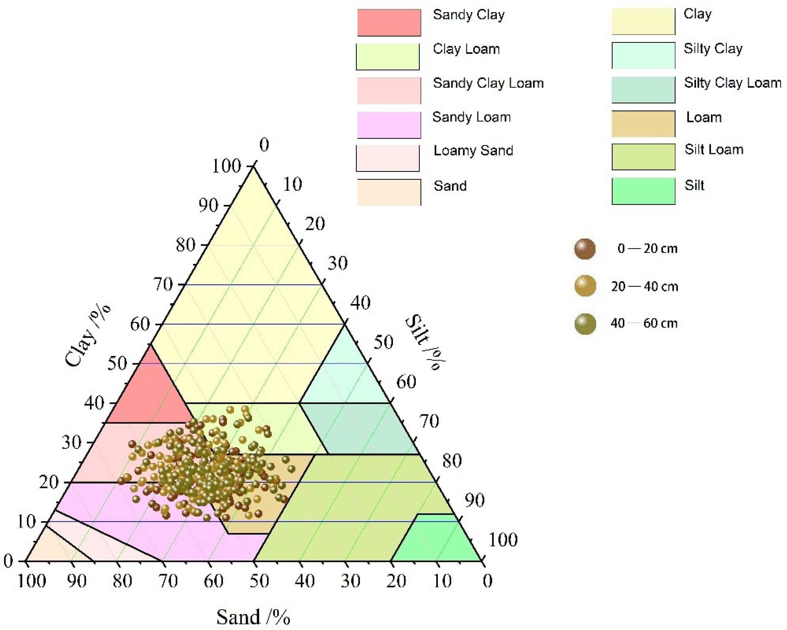
2.2. Soil Sample Collection

According to the vegetation coverage type and soil type distribution characteristics of the study area, a total of 126 plots from May to September 2019 were set up. Soil profiles were dug at each sampling site for soil sample collection. The average depth of soil in the study area is 60 cm; the soil samples were collected at soil layer depths of 10–20 cm, 20–40 cm, and 40–60 cm. Three undisturbed soil cores were taken from the depth of each soil layer to determine K_S (mm min⁻¹) by using ring knifes (Φ 61.80 mm × 56.70 mm), and the average value was taken as the K_S value of the sampling point. Small ring knifes (Φ 50.50 mm × 50.00 mm) were used to collect another three undisturbed soil cores, which were used to measure soil saturated water content (SSWC, cm³ cm⁻³), total porosity (P, %), bulk density (BD, g cm⁻³), non-capillary porosity (P_NC, %), capillary porosity (P_C, %), and field capacity (FC, %). In addition, three portions of disturbed soil (1 per kg) were taken from the same soil layer for determination of organic matter (SOM, %) and mechanical composition (clay (Cl, %), silt (Si, %), sand (Sa, %). In total, 2268 undisturbed soil cores and 1134 disturbed bulk soils were taken back to the laboratory for analysis and measurement. The average of three repeated experiments was used to characterize the soil properties of each soil layer. The physical and chemical properties of 378 soil layers were obtained from 126 plots (

Table 1. Descriptive statistics of soil properties for a total dataset, modeling dataset, and test dataset.

Data	Variables	Minimum	Maximum	Mean	SD	CV (%)
Total (n = 378)	SSWC (cm3 cm−3)	0.26	0.60	0.43	0.07	15.80
	P (%)	42.28	63.39	51.74	4.00	7.73
	BD (g cm−3)	0.89	1.56	1.22	0.11	8.98
	PNc (%)	0.31	18.46	3.70	1.74	46.92
	PC (%)	38.11	58.51	48.04	3.72	7.74
	FC (%)	16.89	60.88	39.81	7.03	17.65
	Cl (%)	10.97	38.47	22.33	5.44	24.36
	Si (%)	8.64	48.97	28.47	7.47	26.25
	Sa (%)	29.98	68.79	49.19	7.68	15.61
	SOM (%)	0.75	4.77	2.63	0.69	26.07
	KS (mm min−1)	0.17	2.17	0.94	0.49	52.45
Modeling (n = 264)	SSWC (cm3 cm−3)	0.26	0.60	0.44	0.07	15.81
	P (%)	42.28	63.39	52.15	4.11	7.88
	BD (g cm−3)	0.89	1.56	1.20	0.11	9.45
	PNc (%)	0.31	18.46	3.76	1.86	49.45
	PC (%)	38.11	58.51	48.39	3.80	7.85
	FC (%)	16.89	60.88	40.64	7.44	18.32
	Cl (%)	10.97	36.24	21.64	5.09	23.52
	Si (%)	8.64	46.69	28.09	7.31	26.03
	Sa (%)	29.98	68.79	50.27	7.51	14.94
	SOM (%)	1.08	4.57	2.75	0.65	23.57
	KS (mm min−1)	0.17	2.17	1.05	0.50	47.13
Test (n = 114)	SSWC (cm3 cm−3)	0.26	0.57	0.41	0.06	14.43
	P (%)	43.52	61.45	50.78	3.58	7.05
	BD (g cm−3)	1.01	1.41	1.26	0.09	6.97
	PNc (%)	1.39	12.95	3.56	1.41	39.50
	PC (%)	39.38	58.15	47.22	3.40	7.20
	FC (%)	24.20	57.40	37.90	5.52	14.57
	Cl (%)	13.36	38.47	23.94	5.89	24.60
	Si (%)	11.66	48.97	29.36	7.79	26.54
	Sa (%)	30.42	67.06	46.70	7.51	16.08
	SOM (%)	0.75	4.77	2.37	0.71	29.76
	KS (mm min−1)	0.17	1.61	0.67	0.37	54.28

SD: standard deviation; C_V: coefficient of variation.

).

2.3. Laboratory Experiment

The saturated hydraulic conductivity (K_S) of undisturbed soil scores was measured by the constant head method [9].

Before measurement, all the soil samples were dried naturally. Soil Organic Carbon (SOC, %) was determined by the potassium dichromate dilution heating method. Soil Organic Matter (SOM, %) can be converted by the following formula:

$$\mathrm{SOM}=\mathrm{SOC}\times 1.724$$

(1)

Particle-size distribution was determined using a Malvin laser particle size analyzer (Mastersizer 2000). Soil texture was classified according to the International Classification of soil texture. Soil samples that were disturbed were dried in an oven at 105 °C for 24 h and weighed to determine their SSWC, P, BD, P_NC, P_C, and FC.

2.4. Data Analysis

Modeling data (n = 264) were used to modify the parameters of the PTFs using the nonlinear least-square method. Test data (n = 114) were used to validate the prediction performance of the modified PTFs. For consistency, modeling data (n = 264) was used to develop the MLR and ANN PTFs, and the test data (n = 114) were used to validate the prediction performance of the newly established PTFs.

2.4.1. Regression Analysis

Multiple Linear Regression (MLR) is a well-established method for the development of Pedo-Transfer Functions to predict the soil hydraulic parameters. Stepwise regression is a common method to avoid multicollinearity in Multiple Linear Regression analysis. Firstly, variables were introduced into the model one by one, and an F test was performed after each explanatory variable was introduced. Secondly, to ensure that only significant variables were included in the regression equation before each new variable was introduced, T-test was performed on the selected explanatory variables one by one when an explanatory variable was introduced and it was significant. However, when the second explanatory variable was introduced, the previously introduced explanatory variable was deleted because it was no longer significant. The explanatory variables finally retained in the model were not only important, but there was also no serious multicollinearity after stepwise regression. Before the multiple regression analysis, the variables (P_NC, FC, Cl, K_S) that did not conform to the normal distribution were converted logarithmically to make them meet the normal distribution.

The basic form of the regression equation was:

$$\mathrm{Y}=\mathrm{a}+{\mathrm{b}}_1{\mathrm{X}}_1+{\mathrm{b}}_2{\mathrm{X}}_2+{\mathrm{b}}_3{\mathrm{X}}_3+\cdots +{\mathrm{b}}_{\mathrm{i}}{\mathrm{X}}_{\mathrm{i}}$$

(2)

where Y is the dependent variable, K_S, a is the intercept; b₁, …, b_i are unstandardized regression coefficients; and X₁, …X_i are independent variables.

Although stepwise multiple regression can be used as a method to solve multicollinearity problems, important variables might be removed in practical applications. For example, variables X₁, X₂, and X₃ had been selected and continued to introduce variable X₄ in the execution process. Due to the multicollinearity problem between X₄ and X₂ and X₃, the variance inflation of X₄ was not significant and was excluded. As a matter of fact, X₄ had a stronger response related to the dependent variable Y, but variable X₄ was perfectly eliminated after the execution of stepwise regression. To solve this problem, it was necessary to consider the possible interaction between variables and quadratic regression when carrying out stepwise multiple regression, so that important variables could be retained as much as possible and the prediction accuracy of the model improved. The formula was as follows:

$$\mathrm{Y}=\mathrm{a}+{\mathrm{b}}_1{\mathrm{X}}_1+\cdots +{\mathrm{b}}_{\mathrm{i}}{\mathrm{X}}_{\mathrm{i}}+{\mathrm{c}}_1{\mathrm{X}}_1{}^2+\cdots +{\mathrm{c}}_{\mathrm{i}}{\mathrm{X}}_{\mathrm{i}}{}^2+{\mathrm{d}}_1{\mathrm{X}}_1{\mathrm{X}}_2+\cdots +{\mathrm{d}}_{\mathrm{i}}{\mathrm{X}}_{\mathrm{i}-1}{\mathrm{X}}_{\mathrm{i}}$$

Stepwise multiple regression was accomplished in SPSS 23.0.

2.4.2. Construction of BP Artificial Neural Network

When two or more highly correlated independent variables are input into the Artificial Neural Network, it will harm the learning ability of the Artificial Neural Network (multicollinearity). Highly correlated inputs mean that the amount of characteristic information presented by each variable is small, so less important variables can be eliminated or new input variables can be sought to replace the old ones. Input variables ensured by stepwise regression were used as the input variables of the ANN to test whether it had better predictive performance than MLR.

The Artificial Neural Network model was established by using MATLAB R2018b. In this study, the new variables extracted from the principal component analysis were taken as the input layer, while K_S was taken as the output layer and the Artificial Neural Network based on the Feed-forward backprop (BP) algorithm used for modeling. In the ANN, the Sigmoid function was selected as the activation function of the input layer, the activation function of the hidden layer was the Tansig function, the Purelin function was the activation function of the output layer, and Trainlm was the training function of the network. The training accuracy was 0.0001, the number of training times was 1000, and the learning rate was 0.01. Training was stopped when the training accuracy was below the set accuracy, or when the maximum number of training times was reached. At present, there is no effective way to determine the number of hidden layers in the Artificial Neural Network. It can only be tested one by one according to the empirical formula:

$$h=\sqrt{m+l}+\alpha$$

where h is the number of hidden layers, m and l are the numbers of the input layer and output layer, respectively, and α is a constant between 1 and 10.

The number of hidden layer nodes was determined by cross-validation. The modeling data were randomly divided into two parts, namely, training data (N = 264) and verification data (N = 114). The training data was used to create the Artificial Neural Network, and the validation data was used to test the error of the model. The number of nodes in the hidden layer with the minimum error was selected as the final model structure.

2.5. Evaluation Criteria of Performance

Two methods are usually used to verify the predicted performance of PTFs. One is the traditional method of statistical comparison of predicted values and measured values of K_S. Another method is a process-based functional verification that uses soil hydraulic parameters to predict water flow through a software program [26]. In this study, the first approach was taken because it can judge the prediction performance of the model well without disturbing the modeling data. For this reason, 264 sample points were randomly selected as modeling data, and the remaining 114 sample points were used as test data to evaluate the prediction effect of the model. To evaluate the predictive performance of PTFs, the following five indicators were selected: (1) the Mean Relative Error (MRE); (2) the Mean Error (ME); (3) the Root Mean Square Error (RMSE); (4) the coefficient of determination (R²); and (5) the Akaike Information Criterion (AIC).

$$\mathrm{MRE}=\frac{1}{n}{\displaystyle \sum }_{n=1}^n\frac{\left|\left(p_i-m_i\right)\right|}{m_i}\times 100\%$$

$$\mathrm{ME}=\frac{1}{n}{\displaystyle \sum }_{i=1}^n\left(p_i-m_i\right)$$

$$\mathrm{RMSE}=\sqrt{\frac{1}{n}{\displaystyle \sum }_{i=1}^n{\left(p_i-m_i\right)}^2}$$

$${\mathrm{R}}^2={\left[\frac{{{\displaystyle \sum }}_{i=1}^n\left(p_i-\overline{p}\right)\left(m_i-\overline{m}\right)}{\sqrt{{{\displaystyle \sum }}_{i=1}^n{\left(p_i-\overline{p}\right)}^2{\left(m_i-\overline{m}\right)}^2}}\right]}^2$$

$$\mathrm{AIC}=2k+n\ln \left({\displaystyle \sum }_{i=1}^n{\left(p_i-m_i\right)}^2\right)$$

where n is the number of the test data, $p_i$ and $m_i$ are the ith predicted value and measure value, respectively (i = 1, 2, 3, …, n), and $\overline{p}$ and $\overline{m}$ are the mean values of the predicted and measured values, respectively. The k is the number of parameters in the PTFs. To achieve a better predictive performance of PTFs, MRE, RMSE, and AIC should be as low as possible, and ME should approach 0 while R² should be close to 1.

3. Results and Discussion

3.1. Descriptive Statistics

The descriptive statistics and variable coefficient of K_S and basic soil parameters for total data, modeling data, and test data are shown in Table 1. For all our samplings, K_S varied between 0.17 and 2.17 mm/min, with an average value of 0.94 mm/min and a medium variation of 52.45%. The average bulk density was 1.22 g/cm³ with a variable coefficient of 8.98%, in the range of 0.89–1.56 g/cm³. The mean of SSWC was 0.43 cm³cm⁻³; this represents the maximum water-holding capacity of the soil, that is, the amount of water in which all the porosities between soil particles are filled with water. The P, which included both P_NC and P_C, varied between 42.28 and 63.39%. The P_C, also known as soil water-holding porosity, ranged between 38.11 and 58.51%, with a variable coefficient of 7.74%. The P_NC, which varied between 0.31 and 18.46%, with a coefficient of variation of 46.92%, was filled by water only when there was a large amount of gravity water, so it was also called the soil air pore or soil aeration pore. Representing the soil mechanical composition, Cl, Si, and Sa had average values of 22.33, 28.47, and 49.19%, respectively. The SOM varied between 0.75 and 4.77%, and its mean value and variable coefficient were 2.63% and 26.07%, respectively.

Among all the measured soil basic parameters, the P had the least variable coefficient (7.73%), while the K_S had the highest variable coefficient (52.64%). As the research results of Arshad et al. show, one of the reasons for the higher variable coefficient of K_S is probably the large study area and obvious spatial heterogeneity [27]. The higher variation degree of parameters may be due to the difference between small-scale and large-scale data fluctuations [7,28].

The texture types of the soil layers 0–20 cm, 20–40 cm, and 40–60 cm at 128 plots in the study area and the International Classification of soil texture are shown in Figure 1. It can be seen that all soil samples collected covered four types of soil texture (sandy clay loam, sandy loam, loam, and clay loam). Sandy clay loam and loam were the main soil texture types in the study area. There was also no obvious heterogeneity of soil texture at different soil depths. Therefore, all soil samples were taken as a whole and a single soil transfer function was adopted instead of calculating soil layers separately when predicting soil saturated water conductivity by PTFs, which can increase the number of samples and improve the prediction accuracy.

As Figure 2 shows, Pearson correlation analysis of 11 soil basic properties demonstrates that, among the 55 variable pairs, 51 pairs were significantly correlated when p ≤ 0.05, and 4 pairs were not. The strongest positive correlations (R > 0.8) were obtained between P and SSWC, P_C and SSWC, P_C and P, FC and SSWC, FC and P, and FC and P_C, while the highest negative correlations (R < −0.8) were observed between BD and SSWC, BD and P, BD and FC, and BD and P_C. K_S had a significant correlation with all variables, and had a moderate positive correlation with SWWC (0.68), P (0.57), P_C (0.54), FC (0.66), Sa (0.71) and SOM (0.66), and a moderate negative correlation with BD (−0.74) and Cl (−0.54).

Exploratory factor analysis was carried out for 10 basic physical and chemical properties of soil by principal component analysis, as shown in

Table 2. Component Matrix after rotating by maximum variance.

	Soil Property	PC1	PC2	PC3	PC4	PC5
Component Matrix	SSWC	0.922	0.189	0.139	0.191	0.163
	P	0.916	0.16	0.099	0.256	0.108
	BD	−0.865	−0.219	−0.19	−0.121	−0.25
	PNC	0.095	0.115	0.035	0.984	0.081
	PC	0.941	0.118	0.09	−0.186	0.08
	FC	0.948	0.153	0.149	−0.003	0.153
	Cl	−0.267	0.067	−0.95	−0.041	−0.14
	Si	−0.166	−0.914	0.344	−0.086	−0.105
	Sa	0.35	0.843	0.337	0.112	0.202
	SOM	0.289	0.204	0.144	0.095	0.917
Eigenvalue		4.536	1.752	1.252	1.151	1.050
Cumulative variance contribution rate		45.358	62.874	75.391	86.899	94.402

. There are generally two selection criteria for principal component factors: (1) select principal component factors with characteristic roots greater than 1.00; (2) select principal component factors with a cumulative contribution rate greater than 85%. The maximum variance method was used to carry out the orthogonal rotation and shows the factor load matrix after rotation. The eigenvalues of the first five principal component factors were greater than 1 and explained 94.402% of the variation of soil properties. The PC1 could explain 45.358% of the variation, and it had high positive loadings from SSWC (0.922), P (0.916), P_C (0.941), and FC (0.948), while having a high negative loading from BD (−0.865). PC1 was named the “pore of soil” component, because it chiefly explained the variations of soil bulk density and pore characteristics. The PC2 explained 17.516% of variation with high negative loading from Si (−0.914) and positive loading from Sa (0.843); hence, PC2 was defined as the “silt and sand” component. The PC3 had a high loading from Cl (−0.95) that explained 12.517% of variation, and it was named the “Clay” component. The PC4 explained 11.508% of variation and had a high loading from P_NC (0.984). PC4 was named the “non-water retention” component because these non-capillary porosity samples have no capillary function and are filled with air. The last PC also had one high loading from SOM (0.917), and it explained 7.503% of variation; PC5 was named the “organic matter” component.

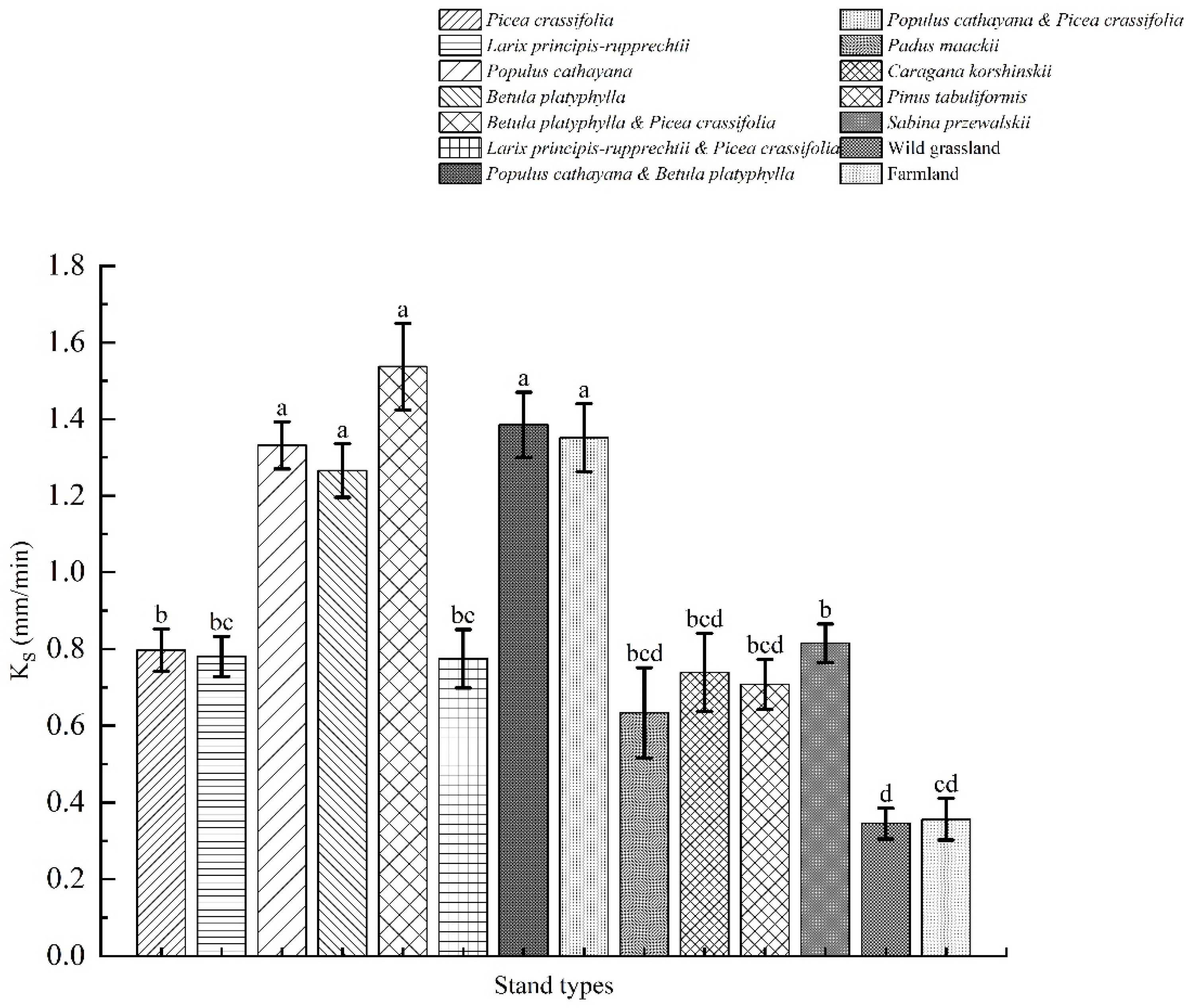
3.2. Characteristics of K_S in Different Stand Types of the Study Area

Comparisons of the average K_S of 14 stand types in the study area were made, and significant difference analysis was conducted, as shown in Figure 3. The saturated water conductivity of the mixed forest of Betula-Picea was significantly higher than that of other stands, but there was no significant difference between it and the mixed forest of Populus-Betula. Farmland and grasslands were significantly lower than most forestland. Rachman et al. and Seobi et al. provided the K_S in vegetation areas, and it can be seen that it is generally higher than that found in farmland [29,30]. The result was not surprising because related studies showed that the K_S of the native natural forest was higher than that of other vegetation types [31]. As the top vegetation community of natural succession in this area, the mixed forest of Betula-Picea had the best water conservation benefits. It is worth mentioning that the K_S of the coniferous pure forest was generally lower than that of coniferous and broad-leaved mixed forest. Lim et al. analyzed 1456 soil samples from South Korea and found that K_S in the broad-leaved mixed forest was significantly higher than that in the coniferous pure forest, which coincides with the results of this study [32]. Firstly, the roots of broad-leaved tree species were more widely spread laterally and produced a large number of small root branches, resulting in more developed soil pores than in coniferous forests [33]. Secondly, the litter of coniferous pure forests did not easily decompose, leading to soil acidification, reducing Soil Organic Matter content and changing soil structure, which is not conducive to the growth of understory vegetation. To increase the K_S, the litter layer could not only increase the organic matter content but also reduce the soil bulk density [34,35]. On the contrary, the soil structure of the coniferous and broad-leaved mixed forest was complex and the vegetation environment was diverse, which results in the difference of K_S. Previous studies have shown that better soil structure and root and pore networks, stronger soil microbial activity, and higher organic matter content can all increase soil saturated water conductivity.

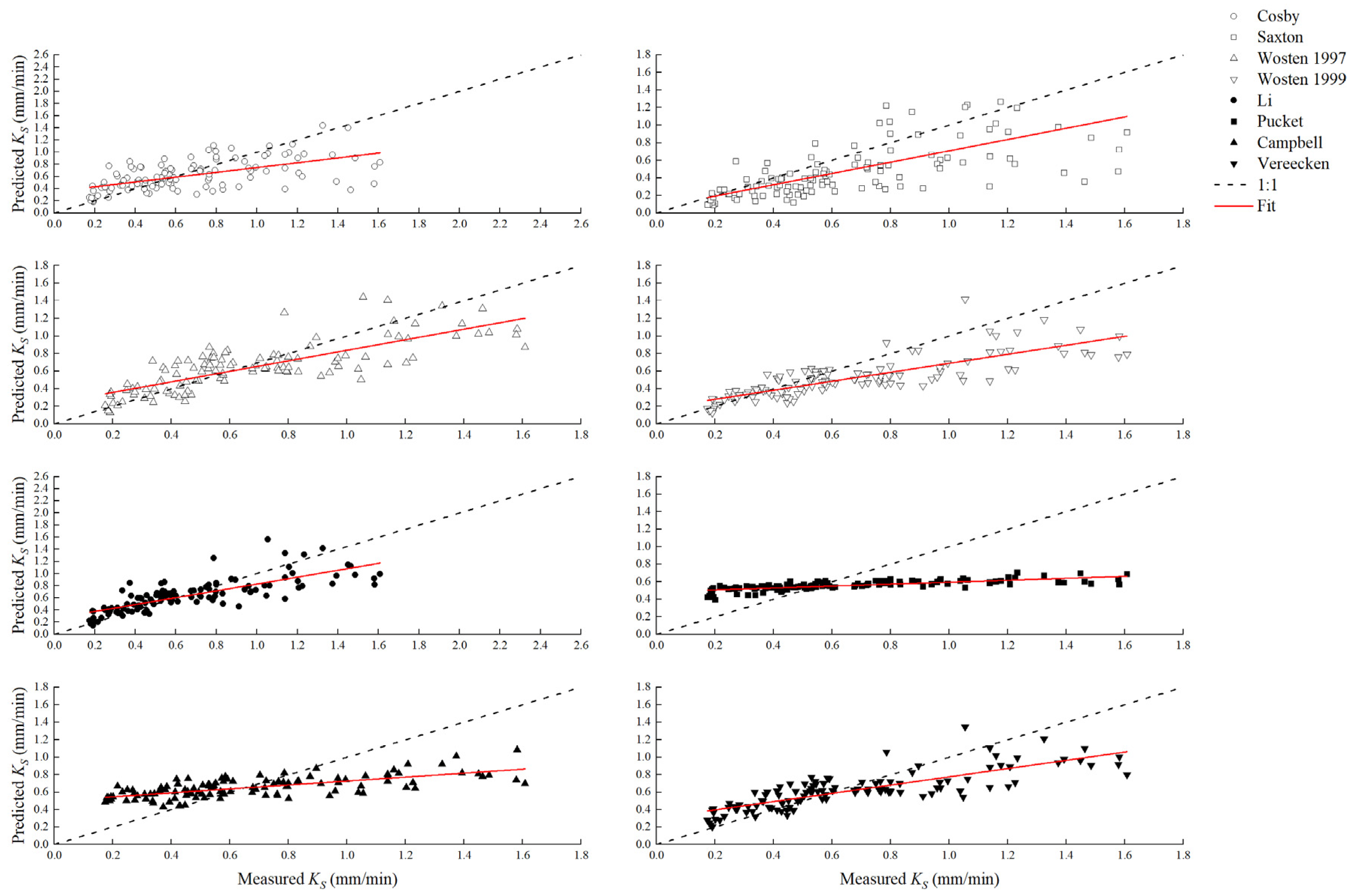
3.3. Modification of the Published PTFs

Currently, many PTFs have been developed with different input parameters and mathematical concepts. These PTFs, however, were established based on linear regression to simulate the relationship between soil hydraulic characteristics and soil basic properties. Based on this, some well-known PTFs were selected that at least contained information regarding soil particle size distribution.

Table 3. Fundamental form of the PTFs modified in this study.

Established PTFs	Input Variables	Formulation
Cosby	Sa; Cl	$\log \frac{K_S}{0.423}=\mathrm{a}+\mathrm{b}·\mathrm{Sa}+\mathrm{c}·\mathrm{Cl}$
Saxton	Sa; Cl; SSWC	$\ln \frac{K_S}{0.16668}=\mathrm{a}+\mathrm{b}·\mathrm{Sa}+\frac{\left(\mathrm{c}+\mathrm{d}·\mathrm{Sa}+\mathrm{e}·\mathrm{Cl}+\mathrm{f}·{\mathrm{Cl}}^2\right)}{\mathrm{SSWC}}$
Wosten 1997	BD; SOM; Cl	$\begin{array}{ll}\ln \frac{K_S}{0.00694}=& \mathrm{a}+\mathrm{b}·\mathrm{BD}+\mathrm{c}·{\mathrm{BD}}^2+\mathrm{d}·\mathrm{SOM}+\mathrm{e}·{\mathrm{SOM}}^2+\mathrm{f}·\ln \mathrm{SOM}+\mathrm{g}·\mathrm{SOM}·\mathrm{Cl}\\ & +\mathrm{h}·\mathrm{BD}·\mathrm{SOM}\end{array}$
Wosten 1999	Si; T; BD; Cl; SOM;	$\begin{array}{ll}\ln \frac{K_S}{0.00694}=& \mathrm{a}+\mathrm{b}·\mathrm{Si}+\mathrm{c}·\mathrm{T}+\mathrm{d}·{\mathrm{BD}}^2+\mathrm{e}·{\mathrm{Cl}}^2+\mathrm{f}·{\mathrm{Si}}^2+\frac{\mathrm{g}}{\mathrm{Si}}+\frac{\mathrm{h}}{\mathrm{SOM}}+\mathrm{i}\ast \ln \mathrm{Si}\\ & +\mathrm{j}·\mathrm{BD}·\mathrm{Cl}+\mathrm{k}·\mathrm{BD}·\mathrm{SOM}+\mathrm{l}·\mathrm{T}·\mathrm{Cl}+\mathrm{m}·\mathrm{T}·\mathrm{Si}\end{array}$
Li	Sa; Cl; SOM; BD	$\ln \frac{K_S}{0.00694}=\mathrm{a}+\mathrm{b}·\ln \mathrm{Sa}+\mathrm{c}·\ln \mathrm{Cl}+\mathrm{d}·\mathrm{Cl}+\mathrm{e}·\ln \mathrm{SOM}+\mathrm{f}·\mathrm{SOM}+\mathrm{g}·\ln \mathrm{BD}$
Pucket	Cl	$\ln \frac{{\mathrm{K}}_{\mathrm{S}}}{1.09}=\mathrm{a}·\mathrm{Cl}$
Campbell	BD; Si; Cl; Sa	$\frac{K_S}{2.4}={\left(\frac{1.3}{\mathrm{BD}}\right)}^{1.3·\mathsf{\alpha }}·\exp \left(\mathrm{a}+\mathrm{b}·\mathrm{Si}+\mathrm{c}·\mathrm{Cl}\right)$ $$\begin{gathered} \mathsf{\alpha }={\left[\exp \left(\mathrm{a}+\mathrm{b}·\mathrm{Si}+\mathrm{c}·\mathrm{Cl}\right)\right]}^{-0.5}+ \\ \mathrm{d}·\exp {\left[\mathrm{e}·\mathrm{Si}+\mathrm{f}·\mathrm{Sa}-{\ln }^2\exp \left(\mathrm{a}+\mathrm{b}·\mathrm{Si}+\mathrm{c}·\mathrm{Cl}\right)\right]}^{0.5} \end{gathered}$$
Vereecken	Cl; Sa; SOM; BD	$\ln \frac{K_S}{0.00694}=\mathrm{a}+\mathrm{b}·\ln \mathrm{Cl}+\mathrm{c}·\ln \mathrm{Sa}+\mathrm{d}·\ln \mathrm{SOM}+\mathrm{e}·\mathrm{BD}$

lists the equation forms of the eight PTFs selected and the required input variables.

Table 4. Results of parameter correction by the least-square method.

Parameter	Cosby	Saxton	Wosten 1997	Wosten 1999	Li	Pucket	Campbell	Vereecken
a	0.378 ± 0.017	1.801 ± 0.036	6.437 ± 0.327	5.916 ± 0.078	4.829 ± 0.131	−0.028 ± 0.002	−1.102 ± 0.064	6.018 ± 0.086
b	0.008 ± 0.001	0.003 ± 0.0007	−0.75 ± 0.321	−0.049 ± 0.016	0.141 ± 0.047		−0.0095 ± 0.0047	−0.176 ± 0.028
c	−0.026 ± 0.002	0.031 ± 0.006	−1.121 ± 0.242	0.076 ± 0.05	−0.234 ± 0.038		−0.0003 ± 0.0055	0.148 ± 0.039
d		0.017 ± 0.004	−0.732 ± 0.435	−1.18 ± 0.192	−0.035 ± 0.05		0.055 ± 0.077	0.649 ± 0.065
e		−0.077 ± 0.01	0.021 ± 0.046	0.00099 ± 0.00058	0.574 ± 0.114		−2.889 ± 0.284	−1.687 ± 0.137
f		0.001 ± 0.0002	0.957 ± 0.193	0.000424 ± 0.000289	0.134 ± 0.073
g			−0.004 ± 0.002	−0.017 ± 0.01	−0.406 ± 0.064
h			0.599 ± 0.205	−0.214 ± 0.028
i				0.344 ± 0.049
j				0.014 ± 0.022
k				0.128 ± 0.037
l				0.0062 ± 0.0059
m				0.0036 ± 0.0048

shows the results of parameter estimation for each PTFs. To evaluate the applicability of these functions in the study area more reasonably, the nonlinear least-square method was adopted to modify the parameters.

Table 5. Predictive performance of the modified PTFs.

Modified PTFs	R2	RMSE	MRE (%)	ME	AIC
Cosby	0.335	0.305	33.717	−0.055	274.970
Saxton	0.460	0.335	34.954	−0.177	302.794
Wosten 1997	0.624	0.226	27.159	−0.032	216.723
Wosten 1999	0.654	0.270	25.022	−0.152	267.629
Li	0.604	0.232	25.957	−0.029	220.600
Pucket	0.561	0.346	42.628	−0.115	299.691
Campbell	0.481	0.295	47.058	−0.02	273.876
Vereecken	0.655	0.235	28.266	−0.052	219.698

shows the estimated and measured values of AIC, R², RMSE, ME, and MRE, calculated using the eight modified Pedo-Transfer Functions of soil saturated water conductivity. From the determination coefficient R², the R² of the Vereecken (0.655) and Wosten 1999 (0.654) PTFs was the largest, which indicated that the predicted value of K_S calculated by these PTF s was closest to the variation trend of the measured value in the study area. The predicted value of the Wosten 1997 PTF had a minimum of RMSE (0.226) and AIC (216.723). From this aspect, the estimation accuracy of the Wosten 1997 PTF was the highest, and the estimation accuracy of the Li and Vereecken functions was also similar to that of the Wosten 1997 PTF. The ME of the predicted value calculated by all PTFs and the measured value were all less than 0, which indicated that the predicted value as a whole was less than the measured value. To further more intuitively understand the prediction effect, Figure 4 shows a comparison of the predicted and measured values of K_S, calculated using eight PTFs. It can be seen that the predicted values of the modified functions of Wosten 1997, Wosten 1999, Li, and Vereecken were basically distributed on both sides of the 1:1 scale line. Yao et al. used the Levenberg–Marquardt algorithm to non-linearly fit the Vereecken function and achieved good prediction results [6]. Tietje and Tapkenhinrichs compared several famous PTFs and believed that the Vereecken PTF had the best prediction performance, while the Saxton PTF had a poor prediction effect for soil with higher organic matter content, which was consistent with the results of this study [36]. In another study, Tietje pointed out that the K_S predicted values of the Saxton, Cosby, and Vereecken PTFs were usually higher than the measured values, which was contrary to the results of this study and might be caused by the correction of model parameters [37]. In summary, functions of the modified Wosten 1997, Wosten 1999, Li, and Vereecken PTFs had a better prediction effect, and they all took SOM as the input variable, while the modified Cosby, Saxton, Pucket, and Campbell functions had a poor prediction effect and did not take SOM into account. Therefore, SOM might be an important variable affecting the prediction accuracy of K_S. In addition to the selection of input variables, inherent variations of K_S, such as measurement error, spatial variability, and sample error, were the reasons for prediction errors of K_S using PTFs [37]. It was therefore necessary to establish a suitable Pedo-transfer function to better predict K_S.

3.4. Multiple Linear Regression

The multiple regression model established by the stepwise regression method was as follows. MLR₁ only considered the primary correlation of variables, while MLR₂ considered the interaction and secondary correlation between variables.

MLR₁:

$$K_S={\mathrm{e}}^{1.101-1.516\mathrm{BD}+0.029\mathrm{Sa}+0.284\mathrm{SOM}-0.533\ln \mathrm{Cl}}$$

MLR₂:

$$K_S={\mathrm{e}}^{2.45+0.011\left(\mathrm{Si}·\mathrm{SOM}\right)-0.047\left(\mathrm{BD}·\mathrm{Si}\right)-0.25{\ln }^2\mathrm{Cl}+{\mathrm{SOM}}^2+\mathrm{SOM}·\ln \mathrm{Cl}}$$

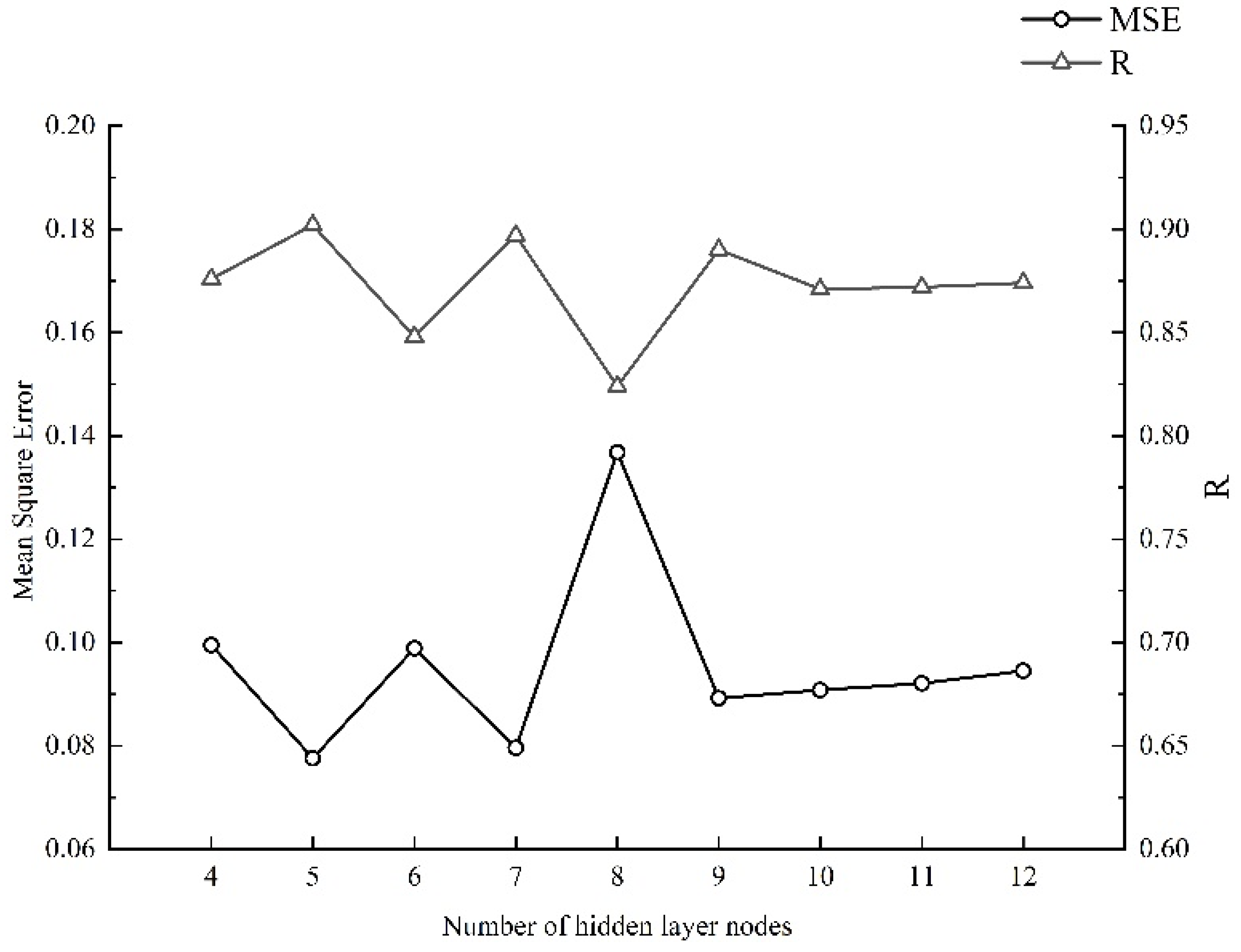
3.5. Development of BP Artificial Neural Network

In order to avoid multicollinearity among input variables, the interaction between soil properties should also be considered. Five variables (x₁ = $\mathrm{Si}·\mathrm{SOM}$, x₂ = $\mathrm{BD}·\mathrm{Si}$, x₃ = ${\ln }^2\mathrm{Cl}$, x₄ = ${\mathrm{SOM}}^2$, and x₅ = $\mathrm{SOM}·\ln \mathrm{Cl}$) were adopted, which were generated by the MLR₂ model as the input layer and $\ln {\mathrm{K}}_{\mathrm{S}}$ as the output layer of the ANN to verify whether it had better predictive performance than MLR₂. The number of hidden layer nodes selected ranged from 4 to 12. Figure 5 shows that the R and MSE of the ANN can be used for predicting soil saturated water conductivity by setting the different numbers of hidden layer nodes. When the number of hidden layer nodes was 5, the ANN had the lowest MSE (0.0776) and the highest R (0.902). Therefore, when the topology of the neural network was 5-5-1, it had optimal prediction performance.

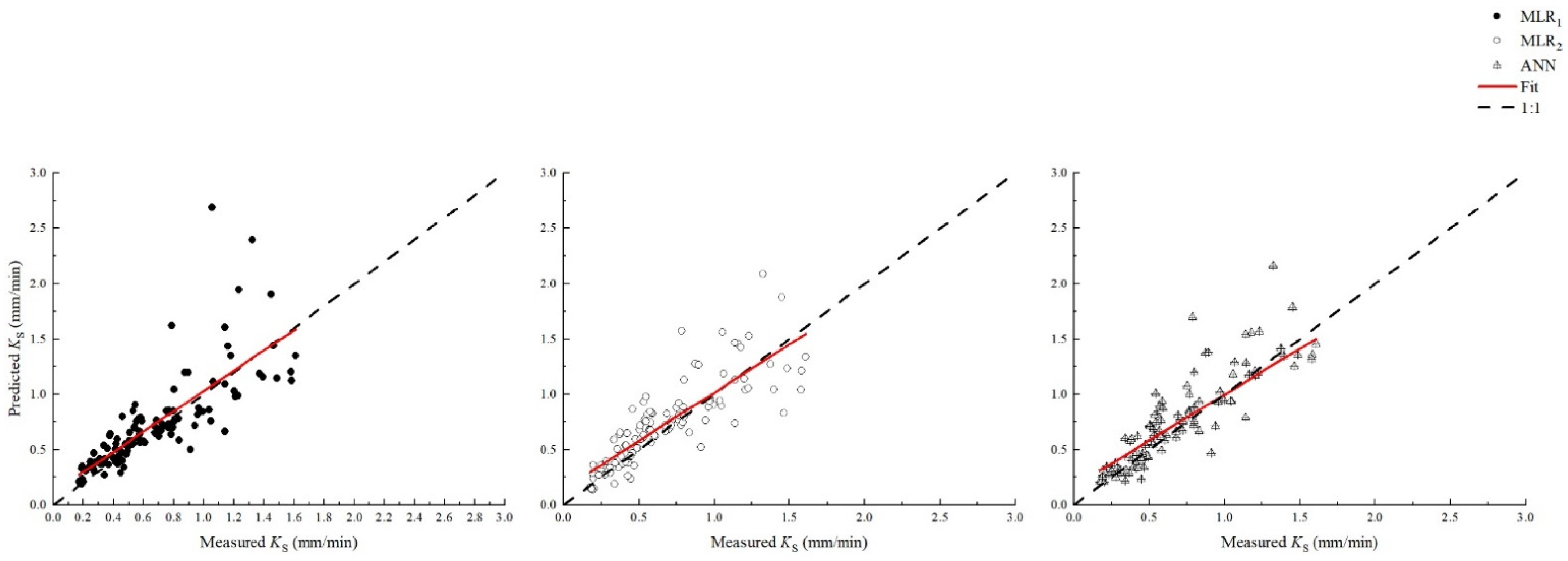
3.6. Evaluation of Prediction Performance of the Model

The 114 data that were not involved in the modeling were used as test data, and they were input into the proposed Multiple Linear Regression equation and the BP Artificial Neural Network to obtain the predicted values of the two models for soil saturated hydraulic conductivity.

As can be seen from Figure 6, the predicted values of K_S of the two models were basically distributed around the 1:1 proportion line, and some points greatly deviated from the 1:1 proportion line, but the overall predicted values were not significantly different from the measured values.

Table 6. Predictive performance of the newly established PTFs.

New PTFs	R2	RMSE	MRE	ME	AIC
MLR1	0.615	0.272	24.900	0.057	255.040
MLR2	0.694	0.223	25.002	0.057	209.812
ANN	0.769	0.209	22.248	0.067	192.610

shows the accuracy information of the two models in predicting soil saturated water conductivity. Compared with MLR₁ and MLR₂, the ANN had a higher R² and a lower RMSE and AIC. However, from the perspective of ME, MLR was lower than the ANN, which was not surprising, because MLR was unbiased. The prediction results of MLR and the ANN were superior to those of the published PTFs in Table 5.

As expected, the prediction performance of MLR₂ was better than that of MLR₁ because MLR₂ retained more useful information, such as Si. Another reason for this was that MLR₂ took into account possible interactions and quadratic correlations between soil properties. The ANN had the highest R² and the lowest RMSE, MRE, and AIC compared to MLR₁ and MLR₂, while ME was only just over 0.01 higher. Therefore, it can be considered that the BP-ANN had higher prediction accuracy than the model established by Multiple Linear Regression. Some scholars believe that Artificial Neural Networks can extract nonlinear information between soil properties, which was not available in Multiple Linear Regression [6]. As stated by Wosten et al., another advantage of Artificial Neural Networks is their ability to mimic the behavior of complex systems by altering the strength of interaction and range of choices of structures of interconnections between every component in a network [7].Compared with the eight previously modified the established PTFs, MLR₂ and ANN had higher predictive accuracy. From the perspective of the prediction results of the model, the difference between the prediction results of MLR and ANN was not only caused by the nature of the model itself (MLR₂ and ANN) but also by the different input variables (MLR₁ and ANN). After considering the interaction between every soil property, the prediction performance of MLR₂ and ANN was significantly higher than that of MLR₁. Although there was no strong multicollinearity between the input variables by stepwise regression, there was more or less of a correlation (even if the correlation was weak, it cannot be ignored) between the soil properties. Therefore, we suggest that the interaction between independent variables should be considered in future modeling work, rather than eliminating all of them in order to avoid collinearity problems.

To some extent, the MLR and ANN established in this study were comparable because they considered all the soil properties measured, and subjectivity was avoided in the selection of input variables. Of course, PTFs based on Artificial Neural Networks are not always better than PTFs built by MLR. Zhao et al. found that the randomness of grouping test data and modeling data had a great impact on the prediction accuracy of PTFs, so that the stability of the ANN was less than MLR when the input variables were the same, although their prediction performance was generally similar in their study on the Loess Plateau of China [18]. Hasan et al. analyzed 195 soil samples from the Erzincan Plains and showed that the accuracy of prediction of K_S by regression was slightly better than that of ANNs, but the experimental results of this study alone did not indicate that regression was always better than ANNs. Better results may be obtained if a better algorithm is used in the ANN [16]. For example, Rezaei Arshad et al. used two different neural network algorithms, namely a Radial Basis Function (RBF) neural network and a Multilayer Perceptual (MLP) model, to predict the soil saturated hydraulic conductivity in southwest Iran, and their prediction performance was both better than that of Multiple Linear Regression [27]. The research results of S. Tamri et al. and I. Yilmaz et al. also showed that an ANN PTF can obtain more reliable prediction results than MLR [38,39]. In contrast to traditional regression models, ANNs do not require a prior regression model that links the input data to the output data, which was often difficult because these models are unknown [40].

In addition to the commonly used linear regression and Artificial Neural Networks, many statistical techniques have been used in the development of PTFs. Lamorski et al. used soil data from Poland to compare PTFs developed by ANN and Support Vector Machine (SVM). They found that the prediction accuracy of two PTFs was roughly similar, and the one developed from the SVM was even higher [41]. Names et al. developed PTFs for 2125 soil samples from the US NRCS soil database using K-Nearest Neighbor methods (KNN), which is another machine algorithm, but the results showed that the predictive performance of KNN and ANN was almost identical [42]. McKenzie et al. and Souza et al. developed PTFs by methods of regression tree and random forest to predict saturated hydraulic conductivity and bulk density, respectively, and provided their predictive performance [43,44]. In addition to the methods already mentioned, there are some statistical techniques, such as Gaussian processes and Naive Bayes Classifiers, that have not been explored in developing PTFs. Some popular deep learning algorithms, such as convolutional neural networks and deep neural networks, are also expected to be widely used in the development of PTFs.

It should be noted that most PTFs are developed using data-driven methods, so their predictive performance is largely dependent on the reliability of soil data. No matter what kind of PTF, they are an indirect method to predict the saturated water conductivity and are based on the direct measurement method. As noted by Wosten et al. and Minasny and Hartemink, the reliability of the data is far more important than the complexity of the model [7,45]. Therefore, while exploring PTFs with more advanced algorithms, we should also devote ourselves to the innovation of direct measurement technology. The modeling data and test data in this study were randomly divided, and the choice of modeling data and test data will have an impact on the prediction effect of PTFs. Therefore, when comparing and selecting PTFs in the future, it is necessary to verify repeatedly to ensure the stability of the PTFs.

4. Conclusions

(1) Sandy clay loam and loam are the main soil types in the three watersheds. Among different vegetation types, the Ks of coniferous and broadleaf mixed forest and broadleaf pure forest were significantly higher than that of coniferous pure forest and shrub forest, while the Ks of wasteland and farmland were the lowest.

(2) In this study, the parameters of eight published PTFs were modified by the least-square method and their prediction accuracy was evaluated. Among them, the Wosten 1997, Wosten 1999, Li, and Vereecken models with SOM as input variables had good prediction accuracy, while the Cosby, Saxton, Pucket, and Campbell models without SOM as input variables had a poor prediction effect. When PTFs are used in this study area, Soil Organic Matter plays an important role in the estimation of Ks.

(3) In this paper, two types of PTFs were established based on Multiple Linear Regression and Artificial Neural Networks, respectively. Our newly created PTFs showed better predictive performance than the published PTFs evaluated earlier. In the regression analysis, we considered the possible interactions between variables and used the stepwise regression method to eliminate redundant variables, so as to avoid the multicollinearity problem while retaining the important variables. The constructed BP Artificial Neural Network model had better prediction performance than Multiple Linear Regression.

It should be pointed out that, in addition to soil properties, stand structure is also an indirect factor affecting K_S in the conversion of farmland to forest areas. In recent years, the northwest alpine region has gradually started to regulate the stand structure of artificial forests (such as supplementary planting of Qinghai Spruce in pure birch forest to promote natural regeneration; selective cutting and supplementary planting were also started for stands with unreasonable stand density. The PTFs we have established may only apply to the current vegetation structure. Whether the PTFs established in the present stage are suitable for the next few years is still to be further explored, regardless of whether the artificial stand is transformed or there is natural succession of the vegetation community. It is necessary to collect more soil information in the future and take into account site conditions and stand structure factors to develop a PTFs that is suitable in both time and scale.

References

1. Montzka, C.; Herbst, M.; Weihermüller, L.; Verhoef, A.; Vereecken, H. A global data set of soil hydraulic properties and sub-grid variability of soil water retention and hydraulic conductivity curves. Earth Syst. Sci. Data 2017, 9, 529–543. [Google Scholar] [CrossRef] [Green Version]
2. Woolhiser, D.A.; Smith, R.E.; Giraldez, J.V. Effects of spatial variability of saturated hydraulic conductivity on hortonian overland flow. Water Resour. Res. 1996, 32, 671–678. [Google Scholar] [CrossRef]
3. Noguchi, S.; Nik, A.R.; Kasran, B.; Tani, M.; Sammori, T.; Morisada, K. Soil physical properties and preferential flow pathways in tropical rain forest, bukit tarek, peninsular malaysia. J. For. Res. 1997, 2, 115–120. [Google Scholar] [CrossRef]
4. Lee, J.H. The Role of Preferential Flow as a Mechanism for Groundwater Contamination; American Geophysical Union: New York, NY, USA, 1988. [Google Scholar]
5. Shirmohammadi, A.; Montas, H.; Bergstrom, L.; Coyne, K.; Wei, S.; Gish, T. Deterministic and stochastic prediction of atrazine transport in soils displaying macropore flow. In Proceedings of the 2nd International Symposium, Ala Moana Hotel, Honolulu, HI, USA, 3–5 January 2001. [Google Scholar]
6. Yao, R.-J.; Yang, J.-S.; Wu, D.-H.; Li, F.-R.; Gao, P.; Wang, X.-P. Evaluation of pedotransfer functions for estimating saturated hydraulic conductivity in coastal salt-affected mud farmland. J. Soils Sediments 2015, 15, 902–916. [Google Scholar] [CrossRef]
7. Wösten, J.H.M.; Pachepsky, Y.A.; Rawls, W.J. Pedotransfer functions: Bridging the gap between available basic soil data and missing soil hydraulic characteristics. J. Hydrol. 2001, 251, 123–150. [Google Scholar] [CrossRef]
8. Reynolds, W.D.; Elrick, D.E. A method for simultaneous in situ measurement in the vadose zone of field-saturated hydraulic conductivity, sorptivity and the conductivity-pressure head relationship. Ground Water Monit. Remediat. 1986, 6, 84–95. [Google Scholar] [CrossRef]
9. Klute, A. Hydraulic conductivity and diffusivity: Laboratory methods. Soil Phys. 1986, 5, 687–734. [Google Scholar]
10. Abdelbaki, A.M. Evaluation of pedotransfer functions for predicting soil bulk density for U.S. Soils. Ain Shams Eng. J. 2018, 9, 1611–1619. [Google Scholar] [CrossRef]
11. Zhang, Y.; Schaap, M.G. Estimation of saturated hydraulic conductivity with pedotransfer functions: A review. J. Hydrol. 2019, 575, 1011–1030. [Google Scholar] [CrossRef]
12. Bouma, J. Transfer functions and threshold values: From soil characteristics to land qualities. In Proceedings of the Workshop on Quantified Land Evaluation Process, Washington, DC, USA, 27 April–2 May 1986; Volume 6. [Google Scholar]
13. Gupta, S.C.; Larson, W.E. Estimating soil water retention characteristics from particle size distribution, organic matter percent, and bulk density. Water Resour. Res. 1979, 15, 1633–1635. [Google Scholar] [CrossRef]
14. Rawls, W.J.; Brakensiek, D.L. An infiltration based runoff model for use with a design store. In Hydraulics & Hydrology in the Small Computer Age; American Society of Civil Engineers: Orlando, FL, USA, 2015. [Google Scholar]
15. Nelson, M.C.; Illingworth, W.T. A Practical Guide to Neural Nets; Addison-Wesley Publishing Company, Inc.: Upper Saddle River, NJ, USA, 1991. [Google Scholar]
16. Merdun, H.; Çınar, Ö.; Meral, R.; Apan, M. Comparison of artificial neural network and regression pedotransfer functions for prediction of soil water retention and saturated hydraulic conductivity. Soil Tillage Res. 2006, 90, 108–116. [Google Scholar] [CrossRef]
17. Motaghian, H.R.; Mohammadi, J. Spatial estimation of saturated hydraulic conductivity from terrain attributes using regression, kriging, and artificial neural networks. Pedosphere 2011, 21, 170–177. [Google Scholar] [CrossRef]
18. Zhao, C.; Shao, M.a.; Jia, X.; Nasir, M.; Zhang, C. Using pedotransfer functions to estimate soil hydraulic conductivity in the loess plateau of china. Catena 2016, 143, 1–6. [Google Scholar] [CrossRef]
19. Lilly, A.; Nemes, A.; Rawls, W.J.; Pachepsky, Y.A. Probabilistic approach to the identification of input variables to estimate hydraulic conductivity. Soil Sci. Soc. Am. J. 2008, 72, 16–24. [Google Scholar] [CrossRef] [Green Version]
20. De Vos, B.; Meirvenne, M.V.; Quataert, P.; Jozef, D.; Muys, B. Predictive quality of pedotransfer functions for estimating bulk density of forest soils. Soil Sci. Soc. Am. J. 2005, 69, 500–510. [Google Scholar] [CrossRef]
21. Mcbratney, A.B.; Minasny, B.; Cattle, S.R.; Vervoort, R.W. From pedotransfer functions to soil inference systems. Geoderma 2002, 109, 41–73. [Google Scholar] [CrossRef]
22. Kaur, R.; Kumar, S.; Gurung, H.P. A pedo-transfer function (ptf) for estimating soil bulk density from basic soil data and its comparison with existing ptfs. Aust. J. Soil Res. 2002, 40, 847–858. [Google Scholar] [CrossRef]
23. C, Y.W.A.B.; B, M.A.S.; C, Z.L.; D, R.H. Regional-scale variation and distribution patterns of soil saturated hydraulic conductivities in surface and subsurface layers in the loessial soils of china. J. Hydrol. 2013, 487, 13–23. [Google Scholar]
24. Hu, W.; Shao, M.A.; Si, B.C. Seasonal changes in surface bulk density and saturated hydraulic conductivity of natural landscapes. Eur. J. Soil Sci. 2012, 63, 820–830. [Google Scholar] [CrossRef]
25. Gao, L.; Shao, M.; Wang, Y. Spatial scaling of saturated hydraulic conductivity of soils in a small watershed on the loess plateau, china. J. Soil Sediments 2012, 12, 863–875. [Google Scholar] [CrossRef]
26. Simunek, J.; Nimmo, J.R. Estimating soil hydraulic parameters from transient flow experiments in a centrifuge using parameter optimization technique. Water Resour. Res. 2005, 41, 297–303. [Google Scholar] [CrossRef] [Green Version]
27. Arshad, R.R.; Sayyad, G.; Mosaddeghi, M.; Gharabaghi, B. Predicting saturated hydraulic conductivity by artificial intelligence and regression models. Isrn Soil Sci. 2013, 2013, 1–8. [Google Scholar] [CrossRef] [Green Version]
28. Zeleke, T.B.; Si, B.C. Scaling relationships between saturated hydraulic conductivity and soil physical properties. Soil Sci. Soc. Am. J. 2005, 69, 1691–1702. [Google Scholar] [CrossRef]
29. Seobi, T.; Anderson, S.H.; Udawatta, R.P.; Gantzer, C.J. Influence of grass and agroforestry buffer strips on soil hydraulic properties for an albaqualf. Soil Sci. Soc. Am. J. 2005, 69, 893–901. [Google Scholar] [CrossRef] [Green Version]
30. Rachman, A.; Anderson, S.H.; Gantzer, C.J. Computed-tomographic measurement of soil macroporosity parameters as affected by stiff-stemmed grass hedges. Soil Sci. Soc. Am. J. 2005, 69, 1609–1616. [Google Scholar] [CrossRef]
31. Hao, M.; Zhang, J.; Meng, M.; Chen, H.Y.H.; Guo, X.; Liu, S.; Ye, L. Impacts of changes in vegetation on saturated hydraulic conductivity of soil in subtropical forests. Sci. Rep. 2019, 9, 8372. [Google Scholar] [CrossRef] [PubMed] [Green Version]
32. Lim, H.; Yang, H.; Chun, K.W.; Choi, H.T. Development of pedo-transfer functions for the saturated hydraulic conductivity of forest soil in south korea considering forest stand and site characteristics. Water 2020, 12, 2217. [Google Scholar] [CrossRef]
33. Burch, W.H.; Jones, R.H.; Mou, P.; Mitchell, R.J. Root system development of single and mixed plant functional type communities following harvest in a pine-hardwood forest. Can. J. For. Res. 1997, 27, 1753–1764. [Google Scholar] [CrossRef]
34. Piaszczyk, W.; Lasota, J.; Błońska, E. Effect of organic matter released from deadwood at different decomposition stages on physical properties of forest soil. Forests 2019, 11, 24. [Google Scholar] [CrossRef] [Green Version]
35. Chen, Y.; Huang, Y.; Sun, W. Using organic matter and ph to estimate the bulk density of afforested/reforested soils in northwest and northeast china. Pedosphere 2017, 27, 890–900. [Google Scholar] [CrossRef]
36. Tietje, O.; Tapkenhinrichs, M. Evaluation of pedo-transfer functions. Soil Sci. Soc. Am. J. 2004, 57, 1088–1095. [Google Scholar] [CrossRef]
37. Tietje, O.; Hennings, V. Accuracy of the saturated hydraulic conductivity prediction by pedo-transfer functions compared to the variability within fao textural classes. Geoderma 1996, 69, 71–84. [Google Scholar] [CrossRef]
38. Tamari, S.; Wsten, J.H.M.; Ruiz-Suárez, J.C. Testing an artificial neural network for predicting soil hydraulic conductivity. Soil Sci. Soc. Am. J. 1996, 60, 1732–1741. [Google Scholar] [CrossRef]
39. Yilmaz, I.; Marschalko, M.; Bednarik, M.; Kaynar, O.; Fojtova, L. Neural computing models for prediction of permeability coefficient of coarse-grained soils. Neural Comput. Appl. 2011, 21, 957–968. [Google Scholar] [CrossRef]
40. Schaap, M.G.; Leij, F.J. Using neural networks to predict soil water retention and soil hydraulic conductivity. Soil Tillage Res. 1998, 47, 37–42. [Google Scholar] [CrossRef]
41. Lamorski, K.; Pachepsky, Y.; Sławiński, C.; Walczak, R.T. Using support vector machines to develop pedotransfer functions for water retention of soils in poland. Soil Sci. Soc. Am. J. 2008, 72, 1243–1247. [Google Scholar] [CrossRef]
42. Nemes, A.; Rawls, W.J.; Pachepsky, Y.A. Use of the nonparametric nearest neighbor approach to estimate soil hydraulic properties. Soil Sci. Soc. Am. J. 2006, 70, 327–336. [Google Scholar] [CrossRef]
43. Mckenzie, N.; Jacquier, D. Improving the field estimation of saturated hydraulic conductivity in soil survey. Aust. J. Soil Res. 1997, 35, 803–827. [Google Scholar] [CrossRef]
44. Souza, E.d.; Fernandes Filho, E.I.; Schaefer, C.E.G.R.; Batjes, N.H.; Santos, G.R.d.; Pontes, L.M. Pedotransfer functions to estimate bulk density from soil properties and environmental covariates: Rio doce basin. Sci. Agric. 2016, 73, 525–534. [Google Scholar] [CrossRef] [Green Version]
45. Minasny, B.; Hartemink, A.E. Predicting soil properties in the tropics. Earth-Sci. Rev. 2011, 106, 52–62. [Google Scholar] [CrossRef]
Figure 1. Soil texture types at all plots in study area.
Agronomy 11 01581 g001
Figure 2. Pearson correlation analysis between KS and soil properties.
Agronomy 11 01581 g002
Figure 3. Analysis of KS significance difference among different vegetation types.
Agronomy 11 01581 g003
Figure 4. Comparison of the predicted and measured values of KS of the modified PTFs.
Agronomy 11 01581 g004
Figure 5. Mean Square Error and R of different hidden layer nodes.
Agronomy 11 01581 g005
Figure 6. Comparison of the predicted and measured values of KS of the new PTFs developed by MLR and ANN.
Agronomy 11 01581 g006