Characterizing Genotype-Specific Rice Architectural Traits Using Smart Mobile App and Data Modeling

Abstract

The quantity and quality of light captured by a plant’s canopy control many of its growth and development processes. However, light quality-related processes are not very well represented in most traditional and functional–structural crop models, which has been a major barrier to furthering crop model improvement and to better capturing the genetic control and environment modification of plant growth and development. A main challenge is the difficulty in obtaining dynamic data on plant canopy architectural characteristics. Current approaches on the measurement of 3D traits often relies on technologies that are either costly, excessively complicated, or impractical for field use. This study presents a methodology to estimate plant 3D traits using smart mobile app and data modeling. Leaf architecture data on 16 genotypes of rice were collected during two crop seasons using the smart-app PocketPlant3D. Quadratic Bézier curves were fitted to leaf lamina for estimation of insertion angle, elevation angle, and curve height. Leaf azimuth angle distribution, leaf phyllotaxis, canopy leaf angle distribution, and light extinction coefficients were also analyzed. The results could be used for breeding line selection or for parameterizing or evaluating rice 3D architectural models. The methodology opens new opportunities for strengthening the integration of plant 3D architectural traits in crop modeling, better capturing the genetic control and environment modification of plant growth and development, and for improving ideotype-based plant breeding.

1. Introduction

The three-dimensional (3D) architecture of a plant affects its ability to compete for resources, such as light and space aboveground as well as water and nutrients belowground [1]. The quantity and quality of light captured by a plant’s canopy control many of its growth and development processes, such as leaf and stem elongation, bud outgrowth, branching or tillering, flowering, and leaf senescence [2,3,4,5].

Plant responses to light quality changes are coordinated at the individual organ level [6], and the molecular mechanisms underpinning a plant’s response to changes in light quality have been well established [3,4]. Plants perceive neighbor-associated changes in light quality and quantity mainly with phytochromes for red and far-red light and cryptochromes and phototropins for blue light [3].

Most of the knowledge on plant photomorphogenesis and photobiology have been gained through experiments in controlled environments. Application of this knowledge for the precision management and engineering of crops under field conditions requires characterization of the light quality signal (blue or red and far-red light) perceived by plant organs within a canopy and quantification of the subsequent responses of plant organs in a stand setting [2,7]. Crop modeling, especially functional–structural modeling, has been considered an important tool in addressing these challenges [7].

Traditional crop models, such as DSSAT [8,9] and APSIM [10], incorporate major plant physiological and soil processes to simulate soil–plant–environment interactions. These models either represent an average plant or plant population over a unit area. They do not consider plants as individual entities with their own developmental patterns and plastic responses to their environment [11], and they usually do not have an explicit representation of the above- and below-ground 3D plant architecture [12].

Functional–structural plant models (FSPMs) integrate a plant’s architecture and processes that underlie its growth and development [13]. Earlier formulations of FSPMs focused on plant 3D architecture but lacked major plant physiological and soil processes [14,15,16], while more recent FSPMs increasingly incorporate plant physiological and soil processes [17,18,19,20]. FSPM modeling provides the possibilities of simulating individual plants and their architectural dynamics in space and time in a stand setting. It can take into account light interception and scattering at the individual leaf level as a function of leaf size, angle, and optical properties, and it can simulate the dynamic change in light quality with regard to red, far-red light, and blue light within a canopy [3].

With continued progress in the genomics of major crops, there has also been an increasing interest in integrating crop modeling across the biological organization from genomics to individual plants to plant populations to communities [21,22]. Combining the physiological strength of traditional crop models with the functional–structural strength of FSPMs offers a great opportunity to better capture the genetic control and environment modification of plant growth and development, which can lead to a greater capability for developing new plant ideotypes or designing precision management strategies for target environments.

A main challenge is the difficulty in obtaining dynamic data on plant canopy architectural characteristics for 3D characterization and for model performance evaluation. Two of the most important architectural traits for rice crop include leaf angle and leaf curvature, which change in relation to leaf position, leaf age, and plant density [23,24,25,26,27,28]. These two traits, along with leaf area index and several other architectural traits, including tiller distribution, leaf phyllotaxis, and leaf azimuth distribution, define a genotype’s canopy structure, affect its canopy light distribution, and play a crucial role in light harvesting and plant productivity [29,30,31,32].

Leaf angle refers to the inclination between the midrib of the leaf blade and the vertical stem of a plant [33], while leaf angle distribution refers to the probability of a leaf element of unit size to have its normal within a specified unit solid angle [32]. Assuming the uniform distribution of leaf azimuth angles, leaf angle distribution becomes the probability density function of the zenith angle of leaf normal [32]. It is one of the most important parameters used to describe the structure of horizontally homogeneous vegetation canopies such as rice. It affects how light is distributed on plant leaves, thus directly affecting plant productivity [32]. Leaf angle distribution has been identified as a key component in developing high-yielding varieties of cereal crops, including rice [33].

Many methods have been developed for estimating leaf angle and/or leaf angle distribution, including inclinometers [34], protractors [27], 3D digitizers [35,36], ground-based digital photography [32,37,38,39,40,41,42,43,44,45], LiDAR (light detection and ranging laser scanning) [46,47,48,49,50,51,52,53,54,55], aerial photography including drones [56,57,58,59], and smartphone photography [43]. Terrestrial LiDAR scanning is increasingly used to measure the canopy structure using point cloud data, which can capture detailed 3D structural information of the canopy [54,55,60,61]. Most of the terrestrial LiDAR studies have been focused on tree canopies, including work by Itakura and Hosoi [51] on isolated tress and Liu et al. [62] on natural beech forest.

A main drawback of terrestrial LiDAR systems is its high cost, making it prohibitive for small budget field campaigns [58]. Photogrammetric methods are limited to outside layers and/or unoccluded objects [58]. Most of the image- and laser-based approaches work poorly in situations where high plant densities are common, such as in rice fields due to excessive object occlusion. PocketPlant3D [63] is a smartphone application that records leaf angles with respect to zenith as the device is moved along the leaf lamina. It has been successfully tested for plant 3D trait estimation in maize [63], rice [64], and common bean [65]. However, detailed methodology and analysis on 3D trait estimation in rice is still lacking. The objectives of this study are to (1) estimate key rice leaf 3D traits using measurements from PocketPlant3D, (2) quantify the effect of genotype, plant density, leaf position, and leaf age on leaf 3D traits, and (3) assess the impact of leaf 3D traits on rice canopy characteristics, including leaf azimuth angle distribution, leaf phyllotaxis, canopy leaf angle distribution, and light extinction coefficients. Existing studies on rice 3D architectural traits have been mainly based on data collected from either protractors [27] or 3D digitizers [28,36,66], representing one or two rice genotypes. This study represents a first comprehensive quantification of the dynamic change in leaf architectural traits of 16 rice genotypes through the rice growing season, based on a smart mobile app and data modeling. The results could be used for breeding line selection or for parameterizing or evaluating rice 3D architectural models. The methodology presented in this paper could also be adapted to 3D architectural research for other Poaceae crops.

2. Materials and Methods

2.1. Experiment Design and Data Collection

A two-year field experiment (16 rice genotypes × two plant densities × three transplanting dates) was conducted at the Texas A&M AgriLife Research Center in Beaumont, Texas (30.0603° N and 94.2934° W) from 2018 to 2019. In 2018, rice was seeded in the greenhouse on 3, 10, and 17 July and the seedlings were transplanted to field plots on 24 July, 31 July, and 7 August, respectively. In 2019, rice was seeded in the greenhouse on 25 April, 9 May, and 23 May and transplanted to field plots on 13 May, 28 May, and 11 June, respectively. Recommended rice production practices were followed to manage the experiment plots (Way et al., 2014). Pesticides were not applied in 2018, but Mustang Maxx was applied to control rice water weevil (Lissorhoptrus oryzophilus) in 2019.

Sixteen rice genotypes were grown each year, consisting of 2 thermogenic male sterile (TGMS) lines, 2 cytoplasmic male sterile (CMS) lines, 2 near-isogenic maintainer (B) lines, 2 restorers (R) lines, 4 TGMS × R hybrids, and 4 CMS × R hybrids (

Table 1. Rice genotypes used in the study.

	Thermogenic Male Sterile		Cytoplasmic Male Sterile
Restorer	212S	279S	119A	339A
170R	212S × 170R	279S × 170R	119A × 170R	339A × 170R
173R	212S × 173R	279S × 173R	119A × 173R	339A × 173R
Maintainers	-	-	119B	339B

). A randomized complete block design was used for this study [67]. A field 35 m wide × 42 m long was divided into 3 equal blocks. Each block was randomly assigned to one of the three transplanting dates. Each block was subdivided into 32 subplots, each randomly assigned to one of the 16 genotypes × two plant densities (5 or 10 plants per meter row with a 20 cm row spacing) combinations. Each subplot had a planting area of 1.0 m × 1.5 m.

In 2018, the three upper most fully expanded leaves from each of 3 tagged main tillers in each subplot were sampled using PocketPlant3D, beginning two weeks after transplanting. Sampling was repeated every 1–2 weeks until flag leaf emergence. In 2019, all fully expanded leaves on 5 tagged main tillers were measured two weeks after transplanting, with leaf length and nodal position recorded with respect to the coleoptile node (node zero). The PocketPlant3D records leaf angle (°) with respect to the zenith and azimuth angles every 200 milliseconds as the device is moved along the leaf lamina. Similar water and fertilizer management were used in both years, and we assumed the same flag leaf nodal position for a genotype in both years.

Four weeks after transplanting in 2019, the uppermost 3–6 fully expanded leaves from a randomly selected tiller in an internal row in each subplot were sampled using PocketPlant3D and then clipped from the insertion point. The clipped leaf blades were placed inside clear plastic bags in a cooler and taken to the lab. The area of each leaf blade was measured with a LI-COR LI 3100 (LI-COR Biosciences, Lincoln, NE, USA), and the length and width of each leaf were measured with a ruler. Individual leaf samples were oven-dried for 3 days at 75 °C, weighed (DL-204, Denver Instrument Company, Arvada, CO, USA), and specific leaf weight (SLW) was calculated as the leaf dry weight (g) divided by the leaf area (cm²). The leaf morphological data (leaf length, width, area, and specific leaf weight) were used to analyze their effect on rice 3D architectural traits.

Temperature data were obtained from the Beaumont Center’s weather station located about 0.8 km from the research field. In 2018, temperatures for rice seedlings while growing inside the greenhouse were estimated by adding a 3 °C adjustment to the outside temperature based on data from Beuzelin et al. [68]. In 2019, temperatures inside the greenhouse were measured with an EM50 data logger and sensors (METER Group, Inc., Pullman, WA, USA). Plant age was calculated as the cumulative degree-days from sowing above a base temperature of 10 °C. Leaf age was calculated as the cumulative degree-days from estimated leaf emergence. To facilitate the graphical comparison of leaf 3D traits among genotypes, leaf node positions were normalized as the current leaf node divided by the flag leaf node position for a genotype, resulting in a value of 1.0 for the flag leaf node position.

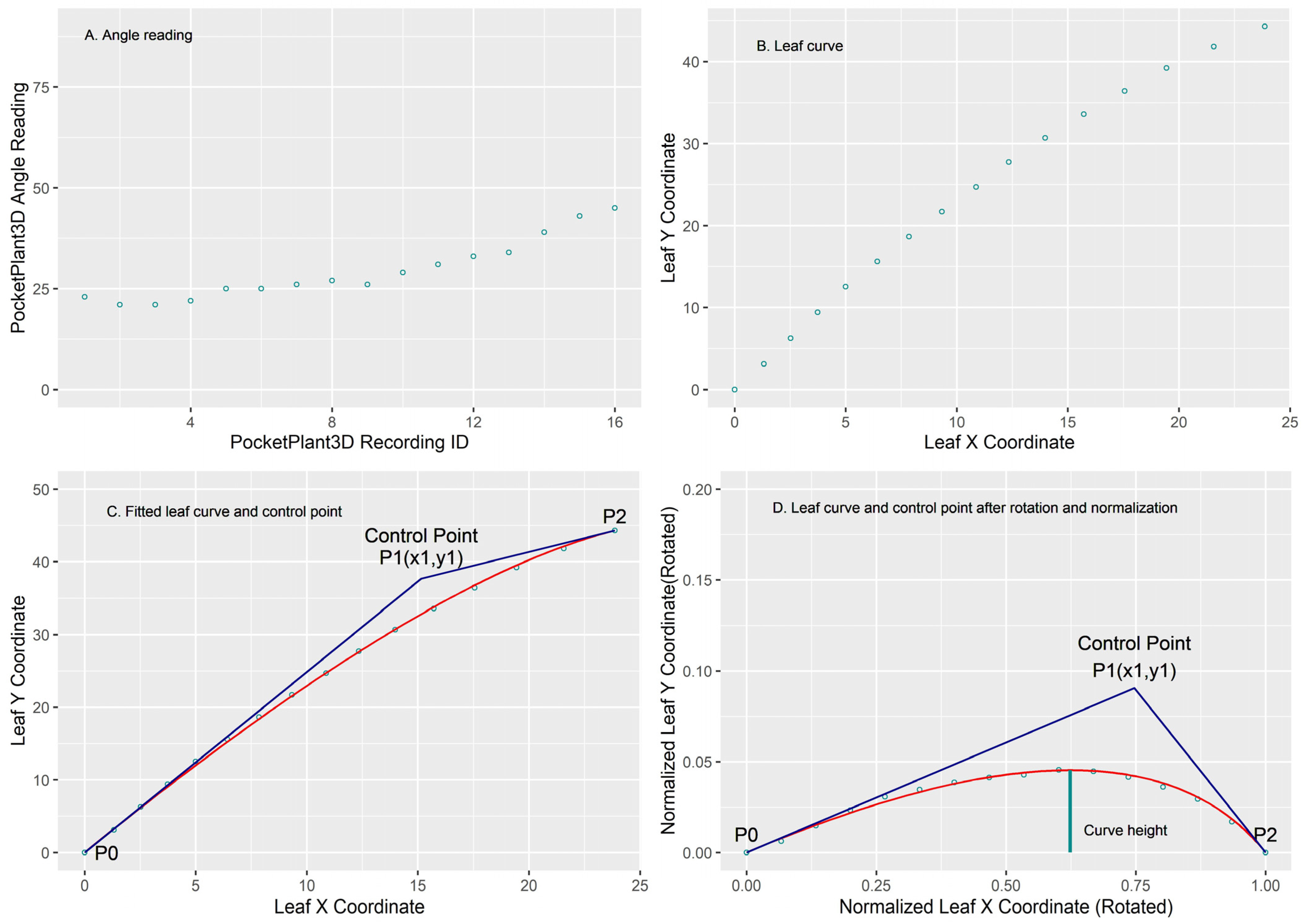
2.2. Calculation of Leaf Insertion Angle, Elevation Angle, and Curve Height

The leaf angles (${\theta }_L$) recorded by PocketPlant3D were converted to a point trace by assuming the phone was moved at a constant speed (Figure 1A) and the total distance traced equal to the leaf length. The length of a leaf segment between two consecutive traced data points ($Lengt{h}_{Segment}$) was calculated as the leaf length divided by the total number of leaf segments for the leaf. The x- and y-coordinate of a segment were calculated as

$$x_{Segment}=\cos ({\theta }_L*\pi /180)*Lengt{h}_{Segment}$$

$$y_{Segment}=\sin ({\theta }_L*\pi /180)*Lengt{h}_{Segment}$$

where ${\theta }_L$ refers to the leaf angle recorded by PocketPlant3D with respect to zenith. Then, the coordinates of the leaf are $(0,0)$ for the leaf base and $({\displaystyle \sum _1^n{x}_{Segment,}}{\displaystyle \sum _1^n{y}_{Segment}})$ for the leaf tip (Figure 1B). This approach assumes the phone was moved in a 2D plane. The leaf shape traced in the 2D plane in combination with the leaf azimuth distribution (see Section 2.3) characterizes the 3D distribution of leaves around the rice culms.

A quadratic Bézier function was used to represent leaf blade shape [69,70,71], and it is defined by an insertion point $P_0(x_0,y_0)$, which is the leaf base, a control point $P_1(x_1,y_1)$, and an endpoint $P_2(x_2,y_2)$, which is the leaf tip (Figure 1C) as described by Equations (1) and (2).

$$X(t)={(1-t)}^2{x}_0+2t(1-t)x_1+t^2{x}_2\begin{array}{ccc}& & \end{array}t\in [0,1]$$

(1)

$$Y(t)={(1-t)}^2{y}_0+2t(1-t)y_1+t^2{y}_2\begin{array}{ccc}& & \end{array}t\in [0,1]$$

(2)

where t is the normalized distance from the base of the leaf to the end of the leaf, following the outline of the leaf. Each leaf was fitted to the quadratic Bézier function with a starting point of $P_0(x_0=0,y_0=0)$ at the leaf base and an endpoint of $P_2(x_2,y_2)$ at the leaf tip where $x_2={\displaystyle \sum _1^n{x}_{Segment}}$ and $y_2={\displaystyle \sum _1^n{y}_{Segment}}$, with n being the number of segments. The control point $P_1(x_1,y_1)$ is estimated through curve fitting. The leaf insertion angle refers to the angle formed between the leaf blade at the insertion point and the vertical culm [63]. The leaf insertion angle was calculated as

$$Angl{e}_{Insertion}=90-\arctan \left(\frac{y_1}{x_1}\right)*\frac{180}{\pi }.$$

The leaf insertion angle characterizes how a leaf is attached to the rice stem, with the control point depending on the leaf curvature, leaf length, and insertion angle. To isolate the leaf curvature characteristics, the axes were rotated and normalized so that the x-axis overlaps with the line formed between leaf base and leaf tip. We have $P_0(x_0=0,y_0=0)$ and $P_2(x_2=1,y_2=0)$ after the rotation (Figure 1D), and the Bézier function is simplified to

$$X(t)=2t(1-t)x_1+t^{2}t\in [0,1]$$

(3)

$$Y(t)={(1-t)}^2{y}_0+2t(1-t)y_{1}t\in [0,1].$$

(4)

The leaf elevation angle is typically defined as the angle between the leaf rachis at its insertion point to the stem and the horizontal plane [31]. In the present study, it is defined as the angle formed between the leaf blade at its insertion point to the stem and the horizontal plane after the axis rotation (i.e., the horizontal line between leaf base and leaf tip after the rotation) (Figure 1D) and was calculated as $Angl{e}_{Elevation}=\arctan \left(\frac{y_{1 (rotated and normalizd)}}{x_{1 (rotated and normalizd)}}\right)\frac{180}{\pi }$.

Curve height is defined as the maximum perpendicular distance from a leaf surface to the line formed between leaf base and leaf tip. The elevation angle and curve height characterize the curvature of a rice leaf. A greater elevation angle indicates greater curvature near the leaf base, and a greater curve height indicates greater leaf bending (Figure 1D). The three leaf 3D traits (leaf insertion angle, leaf elevation angle, and curve height) provide a concise characterization of the 3D architecture of rice leaves.

2.3. Leaf Azimuth Distribution and Leaf Phyllotaxis

The average azimuth angle of the first 3 recorded data points were used to estimate the azimuth angle for the leaf. The frequency distribution of leaves in octants (i.e., 45° angular sections around the plant culm) was calculated to summarize the results. Leaf phyllotaxis was calculated as the difference in the azimuth angles of two consecutive leaves progressing from an older or lower leaf to the next younger or higher leaf.

2.4. Canopy Leaf Angle Distribution and Light Extinction Coefficient

Leaf angles were used to estimate the parameter χ (unitless) of the ellipsoidal leaf angle distribution as described in Equation (5) [72]

$$\chi =-3+{\left(\frac{MTA}{9.65}\right)}^{-0.6061}$$

(5)

where the mean leaf tilt angle (MTA) represents the angle in radians between the normal (i.e., perpendicular plane) to the phone screen and the zenith, and it is the complement of ${\theta }_L$. Parameter χ is the ratio of vertical to horizontal projections of leaves in the canopy. It provides a synthetic representation of the degree of erectness of the leaves [72,73]. The lower the value of χ, the higher the tendency of the distribution to approximate a prolate spheroid (erectophile canopy). The extinction coefficient for solar radiation ($k$, unitless) was estimated using Equation (6) [63,73]:

$$k=\frac{\sqrt{{\chi }^2+{\tan }^2{\theta }_L}}{A}$$

(6)

where $A$ was estimated using Equation (7) [72]:

$$A\approx \chi +1.774{(\chi +1.182)}^{-0.733}.$$

(7)

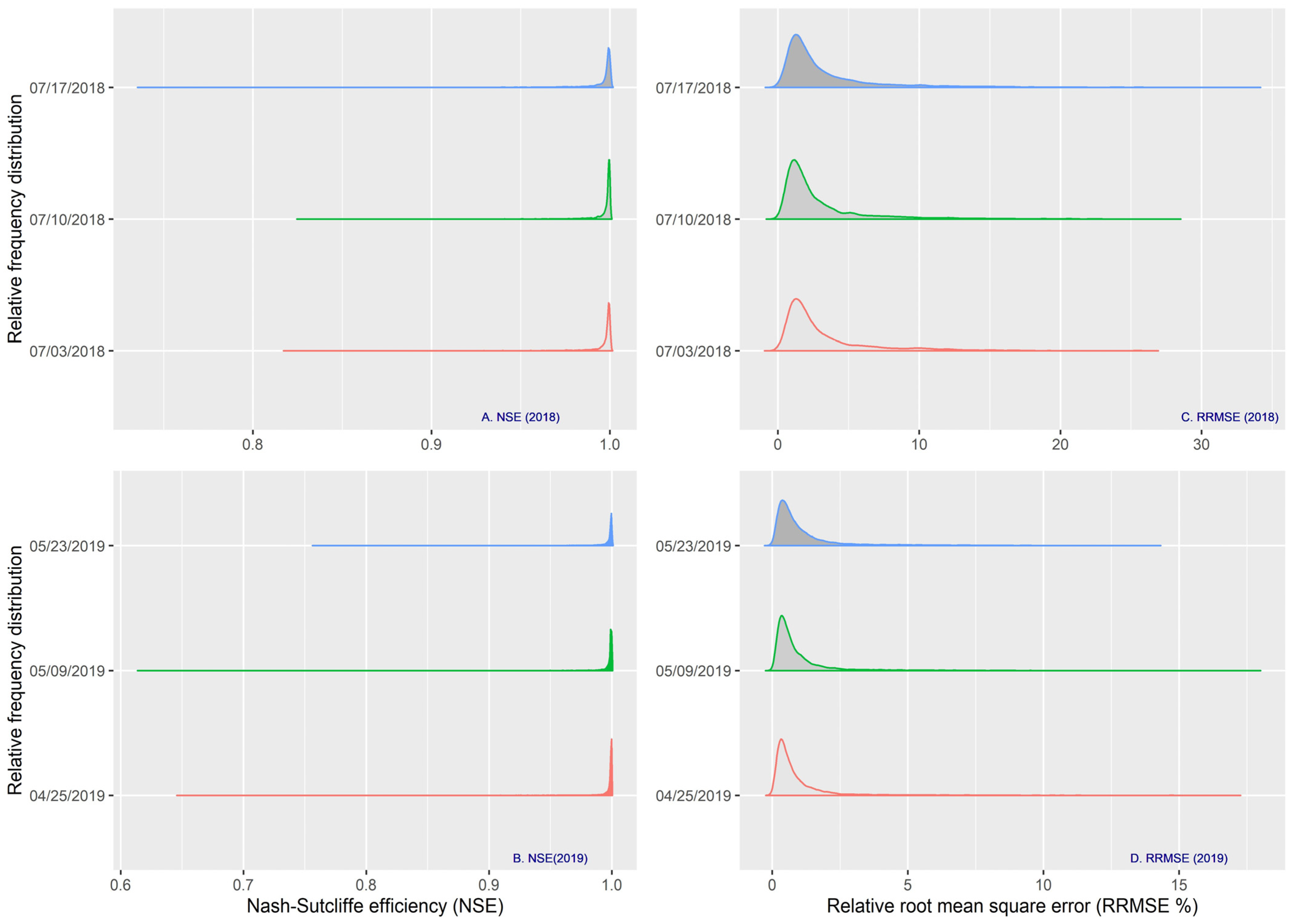
2.5. Curve Fitting and Statistical Analysis

Bézier curve fitting was carried out using a customized version of C# code from GitHub (2019). The agreement between the observed and fitted leaf curves was evaluated using Nash–Sutcliffe efficiency (NSE) [74] and relative root mean square error (RRMSE). Analysis of variance (ANOVA) was conducted using SAS Proc GLM [75], with genotype, density, transplanting time, leaf position, leaf age, and plant age as factors. Leaf and plant ages were converted into categorical variables by grouping data in increments of 200 degree-days, with the mid-point values (e.g., 100, 300, and 500) used as levels.

3. Results

3.1. Analysis of Variance on Leaf Insertion Angle and Leaf Curvature (Elevation Angle and Curve Height)

The shapes of the rice leaves were captured quite well by Bézier curves with mean NSEs of 0.994 and 0.995 and mean RRMSEs of 3.3% and 1.0% for 2018 and 2019, respectively (Figure 2). Figure 3 shows the insertion angle and curvature distribution of leaves at different growth stages for hybrid genotype 212S/173R, which were captured by tracing leaves using PocketPlant3D. Insertion angle decreased at higher leaf positions (lighter-color circles) and curvature increased (more convex) with increasing plant age. Most upper leaves on older plants had smaller insertion angles and much less curvature.

In 2018, each of the five independent variables significantly impacted insertion angle, elevation angle, and curve height (

Table 2. Analysis of variance and percentage of variance explained by main and nested effects for insertion angle, elevation angle, and curve height (field-scanned leaves from tagged plants in 2018 and 2019).

Year	Plant 3D Traits	Variance Explained (%)
		Planting Date	Genotype (PD) 1	Density (PD) 1	Leaf Order (PD G D) 1	Leaf Age (PD G D LO) 1	Total
2018	Insertion angle	8.1 **	7.1 **	0.2 **	25.9 **	22.4 **	63.7
	Elevation angle	13.5	3.8 **	0.1 *	28.6 **	8.9 **	54.9
	Curve height	11.6 **	5.6 **	0.3 **	31.4	8.0 *	56.8
2019	Insertion angle	0.1 **	5.2 **	0.1	8.8 **	18.4 **	32.6
	Elevation angle	1.7 **	1.9 **	0.2 **	12.9 **	7.2 **	23.8
	Curve height	2.0 **	2.6 **	0.4 **	15.5 **	6.3 **	26.9

¹ PD: Planting Date; G: Genotype; D: Density; LO: Leaf order as normalized leaf position; Leaf age as leaf age class; (): Nested ANOVA notation as in SAS. * Significant at p = 0.05; ** significant at p = 0.01. Model and error degrees of freedom for the ANOVA analysis were 763 and 3154, respectively.

). Leaf order (i.e., relative node position) explained the most variability, which is followed by leaf age for insertion angle and planting date for elevation angle and curve height. In 2019, leaf age had the greatest impact on insertion angle and leaf order had the greatest impact on elevation angle and curve height. The impact of planting date on all 3D traits decreased greatly in 2019, while plant density had a marginal but significant impact in both years except for insertion angle in 2019 (Table 2).

Analysis based on measurements from clipped leaves in 2019 indicated that each of the four leaf morphological traits (leaf length, width, area, and specific leaf weight) had a significant impact on elevation angle and curve height except for leaf area, while leaf length was the only morphological trait that significantly impacted insertion angle (

Table 3. Analysis of variance and percentage of variance explained by main and nested effects for insertion angle, elevation angle, and curve height (field-scanned and then destructively clipped leaves from randomly selected plants in 2019).

Plant 3D Traits	Variance Explained (%)
	Planting Date	Genotype (PD) 1	Density (PD) 1	Leaf Order (PD G D) 1	Leaf Age 2	Leaf Length 2	Leaf Width 2	Leaf Area 2	Specific Leaf Weight 2	Total
Insertion angle	0.1	9.9 **	0.2	25.3 **	36.9 **	11.1 **	5.3	4.8	2.6	96.2
Elevation angle	2.2 **	4.8 **	0.0	25.8 **	22.7 *	14.0 **	11.1 **	9.4 **	5.4 **	95.4
Curve height	1.6 **	7.4 **	0.0	29.9 **	16.8	13.6 *	12.7 **	6.6	6.1 *	94.7

¹ PD: Planting Date; G: Genotype; D: Density; Leaf age as leaf age class; (): Nested ANOVA notation as in SAS.; ² Nested ANOVA (PD G D); * Significant at p = 0.05; ** significant at p = 0.01. Model and error degrees of freedom for the ANOVA analysis were 1355 and 121, respectively.

). Similar to field-scanned leaves (Table 2), the leaf order and leaf age had the greatest impact on leaf 3D traits for the clipped leaves (Table 3), which was followed by genotype and planting date. Density had no significant impact on any of the leaf 3D traits. Together with the four leaf morphological traits, these factors explained over 94% of the variability in insertion angle, elevation angle, and curve height (Table 3).

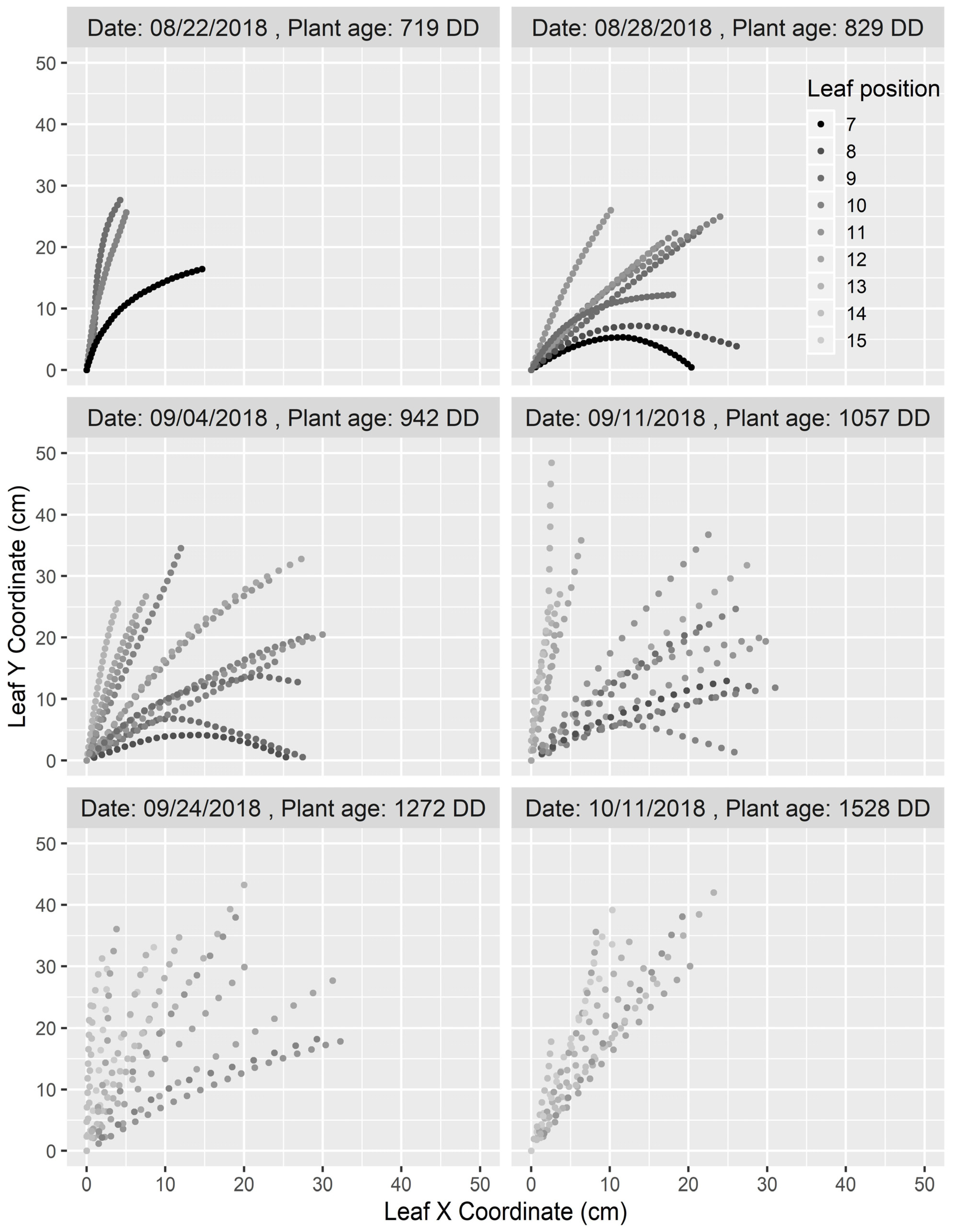
3.2. Dynamics of Leaf Insertion Angle

Leaf insertion angle differed significantly across the three planting dates in 2018 but not between the first and second planting dates in 2019 (Figure 4A,B). The average insertion angle in 2018 was 5.6° less than for 2019, which was probably due to the higher relative leaf order in 2018 (0.71) than in 2019 (0.57), with higher-order leaves being more erect. Average insertion angles were less at the high transplanting density of 10 plants per meter-row in both years, indicating more erect leaves at the higher density, but the difference was significant only in 2018 (Figure 4C,D). There was a strong trend of decreasing insertion angles with increasing leaf order (i.e., for leaves in higher nodal positions) (Figure 4E,F) and a strong trend of increasing insertion angle with increasing leaf age (Figure 4G,H). In 2018, there was a general trend of decreasing insertion angle with increasing plant age (Figure 4I). The insertion angle tended to increase early in 2019 and then slightly decreased for the oldest plant sample (Figure 4J). Average insertion angles among the genotypes ranged from 14.3 to 25.0° in 2018 and 18.3 to 28.5° in 2019, indicating relatively small variation in insertion angles among the genotypes (Figure 4K,L). Insertion angles for the genotypes formed two general groups consistent for both years: (1) small insertion angles (more erect) for 119A-B and 339A-B parents and hybrids developed from crosses with 119A or 339A male sterile parents, and (2) large insertion angles (less erect) for 173R, 212S, and 279S male sterile parents, and hybrids developed from crosses with 212S or 279S parents.

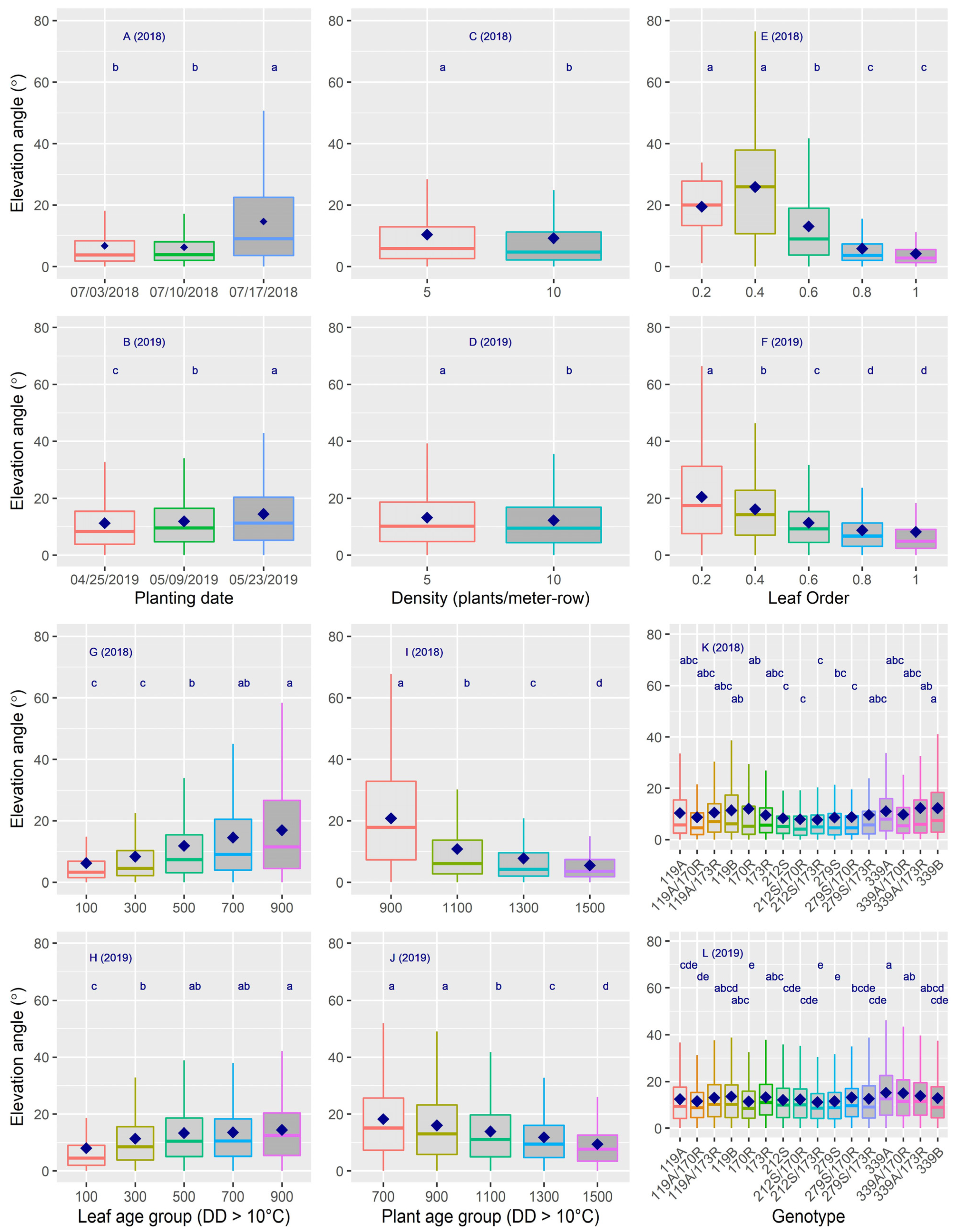
3.3. Dynamics of Leaf Elevation Angle

Elevation angle tended to increase with later planting in both years (Figure 5A,B). The higher elevation angle for later planting dates was due to the inclusion of lower-position leaves. Average leaf orders were 0.71, 0.73, and 0.6 in 2018 and 0.62, 0.61, and 0.51 in 2019 for the first, second, and third plantings, respectively, with a value of 1.0 indicating the flag leaf. Plant density had a small but significant effect on elevation angle in both years (Figure 5C,D), with less elevation angle at the higher density. There were strong trends of decreasing elevation angle with increasing leaf order (Figure 5E,F), increasing elevation angle with increasing leaf age (Figure 5G,H), and decreasing elevation angle with increasing plant age (Figure 5I,J). The trend in elevation angle change in relation to leaf and plant ages was more pronounced in 2018 than in 2019. The elevation angle among genotypes ranged from 7.7 to 13.6° in 2018 and from 11.1 to 15.3˚ in 2019 (Figure 5K,L), with 212S/173R having the lowest elevation angle.

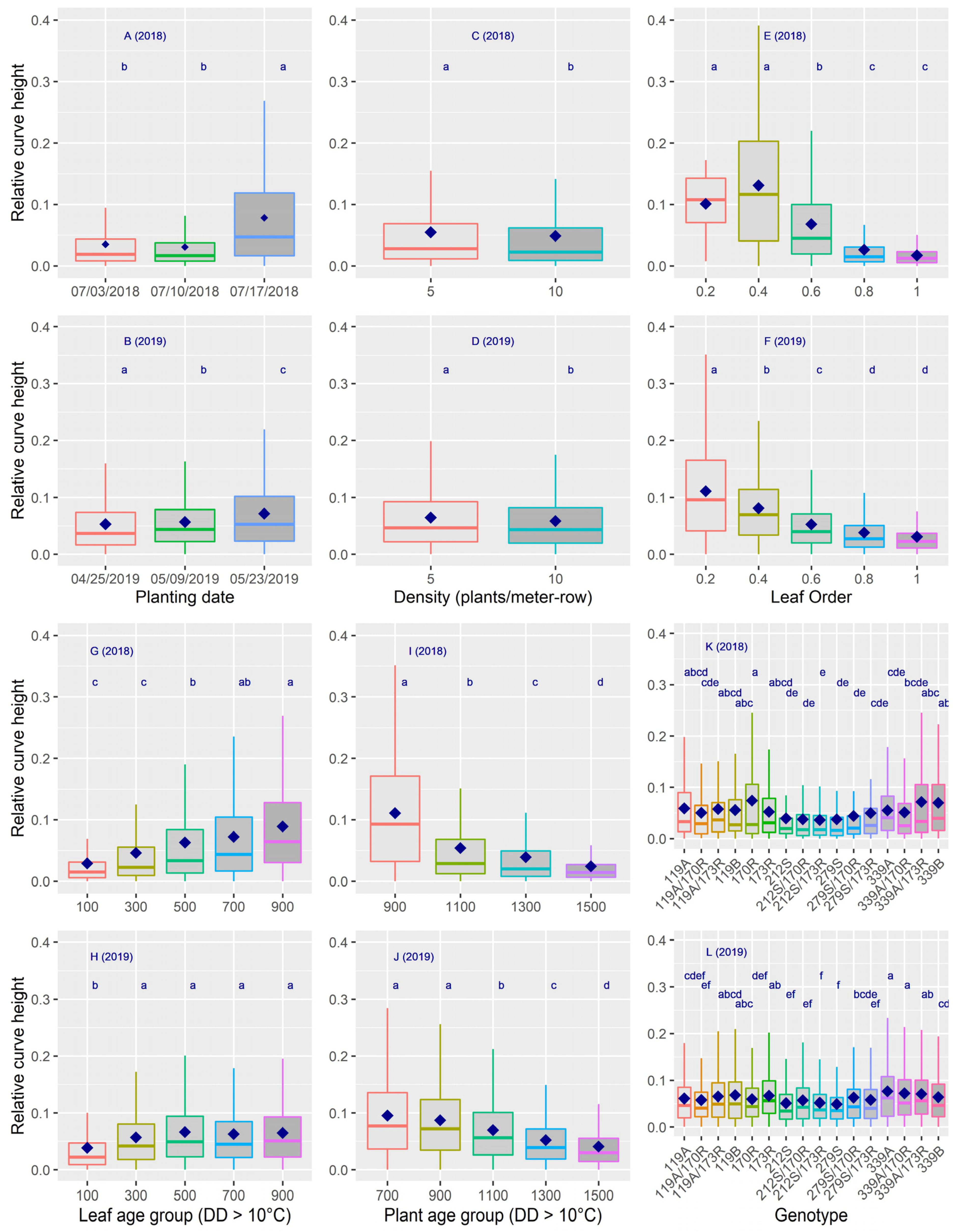
3.4. Dynamics of Curve Height

Increased curve height was observed for later planting (Figure 6A,B), which was due to a greater number of lower-position leaves being present at sampling. Density had a small but significant effect on curve height in both years, with less curve height at the higher density (Figure 6C,D). There were strong trends of decreasing curve height with increasing leaf order (Figure 6E,F), increasing curve height with increasing leaf age (Figure 6G,H), and decreasing curve height with increasing plant age (Figure 6I,J). The trend in curve height change in relation to leaf and plant ages was more pronounced in 2018 than in 2019.

Curve height varied significantly with genotypes (Figure 6K,L), with 279S and 212S/173R having the lowest curve height in both years. The genotypes with the highest elevation angles varied between years, but the general patterns remained similar between the two years. Elevation angle and curve height for the genotypes formed two groups consistent for both years: (1) higher elevation angle and greater curve height (more curved) for 119A-B and 339A-B parents and hybrids developed from crosses with 119A or 339A male sterile parents, and (2) lower elevation angle and less curve height curve height (less curved) for 173R, 212S, and 279S male sterile parents, and hybrids developed from crosses with 212S or 279S parents. This grouping among genotypes is consistent with what was observed for the insertion angle: Genotypes with more erect leaves at the insertion point tended to be more curved, which was probably due to the combined impact of leaf length, width, specific leaf weight, and gravity.

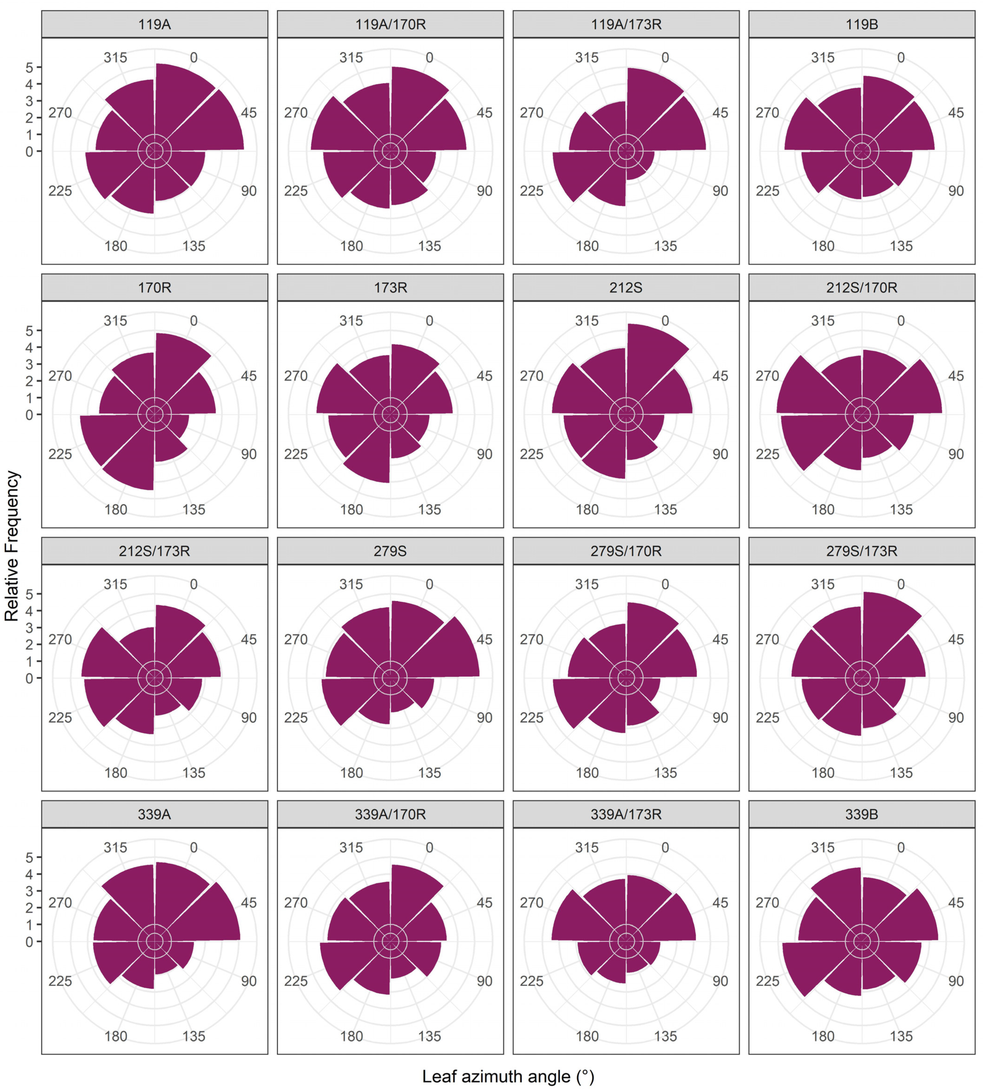
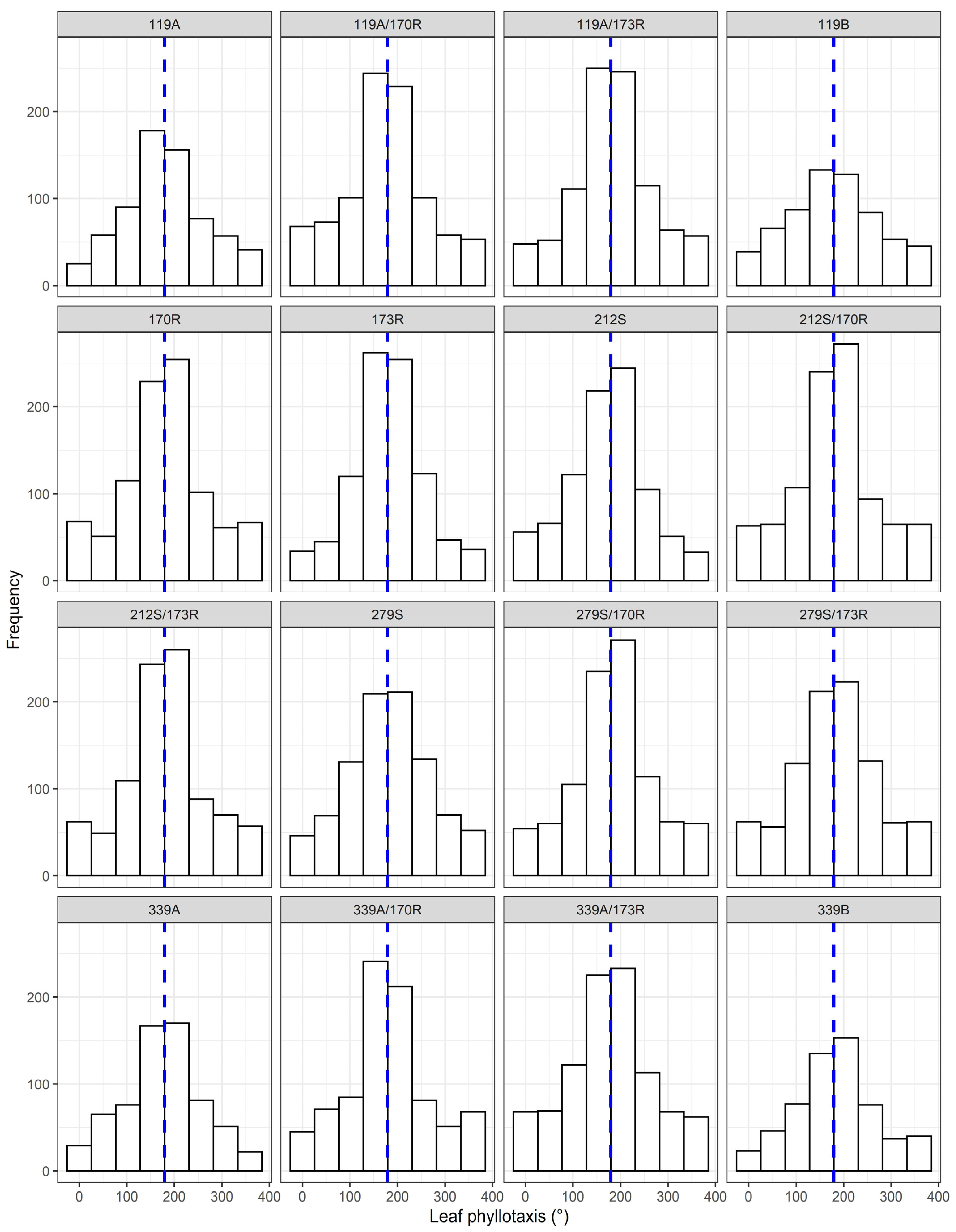
3.5. Leaf Azimuth Distribution and Leaf Phyllotaxis

The distribution of leaf azimuth angles was most significantly impacted by its octant position, which was followed by genotypes, with density and planting date having no significant effect (

Table 4. Analysis of variance for leaf azimuth angle and phyllotaxis as affected by planting date, genotype, density, and octant or leaf order.

Plant 3D Traits	Year	Variance Explained (%)
		Planting Date	Genotype (PD) 1	Density (PD) 1	Octant (PD G D) 1	Leaf Order (PD G D LO) 1	Total
Azimuth angle	2018	0.2	3.9 **	0.1	41.6 **	-	45.8
	2019	0.4	2.48 **	0.1	30.7 **	-	33.7
Phyllotaxis	2018	0.1	1.9	0.1	-	4.2	6.2
	2019	0.0	0.3	0.0	-	1.0	1.3

¹ PD: Planting Date; G: Genotype; D: Density; LO: Leaf order as normalized leaf position; (): Nested ANOVA notation as in SAS. ** significant at p = 0.01. Model and error degrees of freedom for ANOVA analysis on leaf azimuth angles were 713 and 1331 in 2018 and 767 and 3832 in 2019, respectively. Model and error degrees of freedom for ANOVA analysis on leaf phyllotaxis were 144 and 2481 in 2018 and 146 and 10968 in 2019, respectively.

and Figure 7). The uneven distribution was probably due to tiller arrangement within a rice plant and its spatial relationship with adjacent plants. On the other hand, leaf phyllotaxis was not significantly impacted by planting date, genotype, density, and leaf order (Table 4). These four factors explained only 6.2% and 1.3% of the observed variability in leaf phyllotaxis in 2018 and 2019, respectively. The frequency distribution of leaf phyllotaxis had an approximately normal distribution for all genotypes with an average phyllotaxis of 180° for pooled data across years, planting dates, genotypes, and densities (Figure 8); however, the distribution curves were relatively flat, indicating large variation in leaf phyllotaxis.

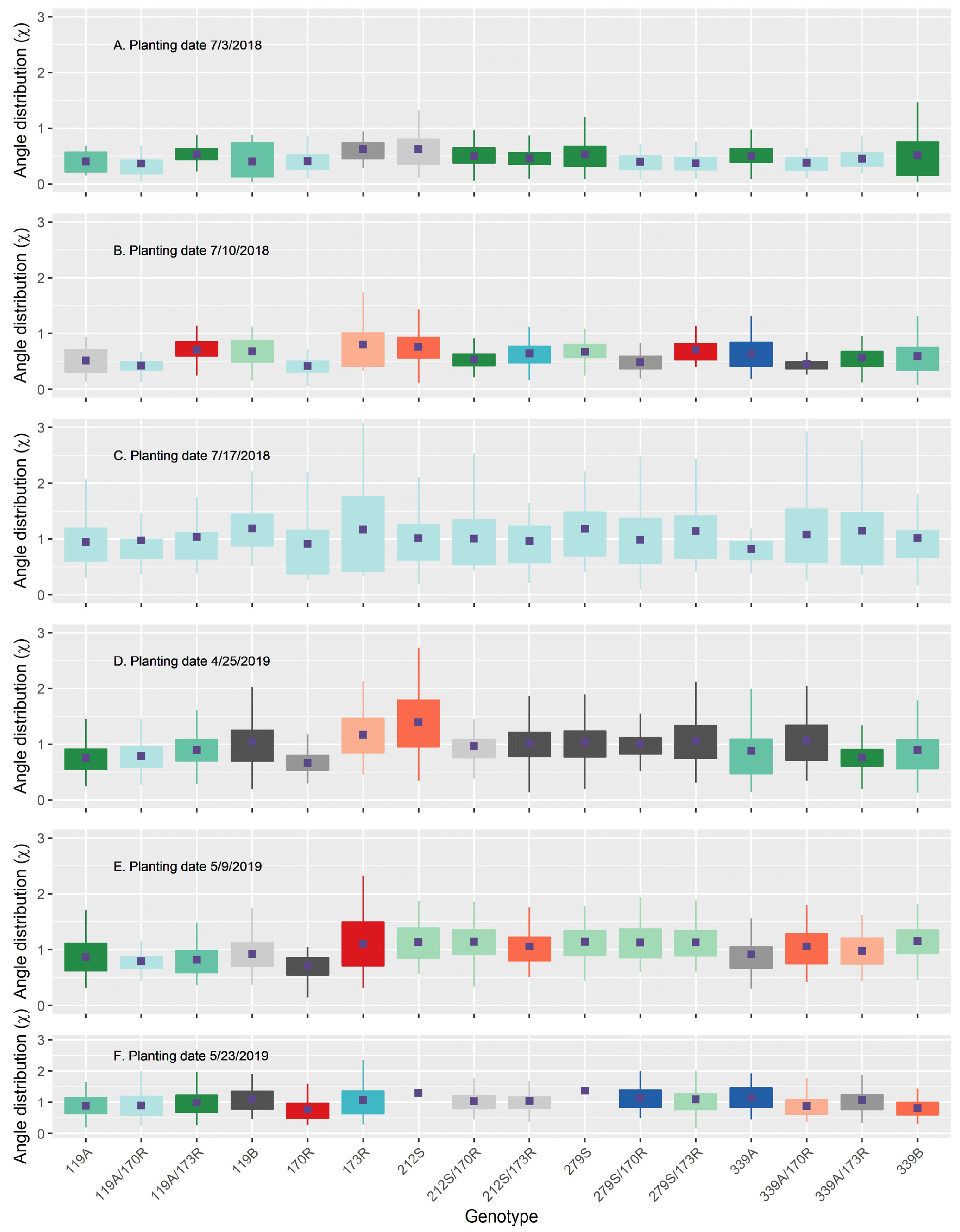
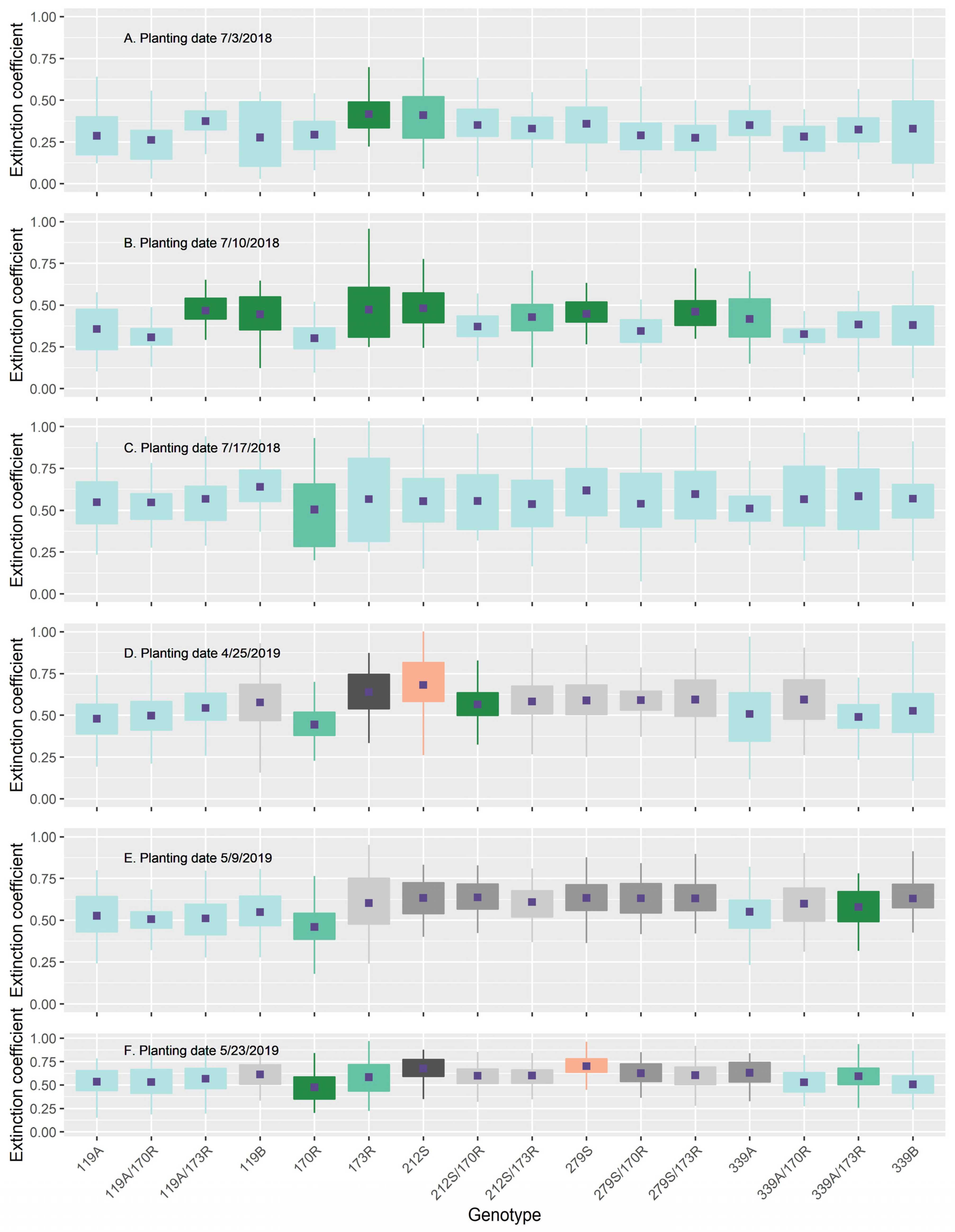
3.6. Canopy Leaf Angle Distribution and Light Extinction Coefficient

Analysis of variance showed significant effects on canopy leaf angle distribution and light extinction coefficient by planting date, genotype, and density, indicating the dynamic nature of canopy structure (

Table 5. Analysis of variance for canopy leaf angle distribution and light extinction coefficient as affected by planting date, genotype, and density.

Plant 3D Traits	Year	Variance Explained (%)
		Planting Date	Genotype (PD) 1	Density (PD) 1	Total
Leaf angle distribution	2018	24.0 **	4.4 **	0.3 *	28.7
	2019	0.5 **	14.4 **	0.9 **	15.7
Light extinction coefficient	2018	27.5 **	6.7 **	0.5 **	34.6
	2019	0.6 **	15.3 **	0.8 **	16.7

¹ PD: Planting Date; (): Nested ANOVA notation as in SAS. * Significant at p = 0.05; ** significant at p = 0.01. Model and error degrees of freedom for ANOVA analysis were 50 and 2167 in 2018 and 50 and 4394 in 2019, respectively, for leaf angle distribution as well as for light extinction coefficient.

). The average leaf angle distribution values (χ) among the genotypes ranged from 0.37 to 1.18 in 2018 and from 0.66 to 1.39 in 2019 (Figure 9). The corresponding light extinction coefficients ranged from 0.26 to 0.64 in 2018 and from 0.44 to 0.70 in 2019 (Figure 10). Ranking in light extinction coefficient among genotypes varied among different planting dates. Genotype 170R consistently had the lowest average light extinction coefficient, while 119B, 212S, and 279S were among the top three genotypes with the largest light extinction coefficients in at least three out of the six planting dates in 2 years (Figure 10).

4. Discussion

This study provided a comprehensive analysis on the impact of plant density, plant age, leaf age, leaf position, genotype, and leaf morphological characteristics on leaf 3D architectural traits. The results could serve as a foundation for building functional–structural plant models critical to analyzing and designing plant types that optimize light harvesting and productivity.

4.1. Rice Leaf Curvature Modeling

Rice leaf curvatures have been described by a number of functions, including Bézier and quadratic curves [69], Bézier surface [76], and Hermite curves [36]. Watanabe, Hanan, Room, Hasegawa, Nakagawa, and Takahashi [36] described rice leaf blade curvatures using three axial angles, with the first axial angle representing leaf insertion angle. Shi, Zhu, and W.X. [66] developed a model for rice leaf curvature characteristics, taking into consideration leaf angle, length, width, specific leaf weight, and deformation coefficient. The model dynamically simulates curvatures of leaves with different leaf angles and specific leaf weights. Yang et al. [69] used a quadratic function to describe leaf mid-vein curvature in 3D space and further expanded the function to account for leaf twisting around the midvein. Liu et al. [77] developed a parabolic leaf vein curve model, considering the vein curve as an arbitrary particle trajectory, involving three parameters that define the leaf vein shape [78]. Dornbusch et al. [79] developed a dynamic leaf curvature model for spring barley, involving eight parameters, which was then adopted by Zhang et al. [28] to develop a dynamic rice curvature model in 3D space, using normalized thermal time. Confalonieri et al. [63] used the mean coefficient of variation of the angles measured by PocketPlant3D for each leaf as a synthetic indicator of leaf curvature.

In this study, we used a quadratic Bézier function to describe rice leaf blade shape and derived three leaf 3D traits, including leaf insertion angle, leaf elevation angle, and curve height. Then, we conducted a comprehensive analysis on how the 3D traits are impacted by genotype, density, leaf age, plant age, and leaf position. These 3D leaf traits provide a concise characterization of the 3D architecture of rice leaves. They could be used to select the best plant types for breeding and cultivation [80] and to strengthen physiologically based functional–structural plant modeling through a detailed characterization of leaf 3D architecture.

4.2. Leaf Angle Dynamics and Distribution Pattern

Leaf angle is determined by the shape of the lamina joint connecting the leaf blade and sheath [81]. Zhou et al. [82] reported that successive cell division and expansion, cell wall thickening, and programmed cell death at the adaxial or abaxial sides form the cytological basis of the lamina joint, and an increased leaf angle results from the asymmetric cell proliferation and elongation. Based on an analysis of 60 maize hybrids released over a span of 65 years, Perez et al. [83] showed that maize leaf erectness tended to decrease with days after sowing for all hybrids. They also reported that the average vertical plane of plants tends to orient toward a direction perpendicular to plant rows, but a high plant-to-plant variability was observed with very low heritability.

Based on the ideotype concept [84], upright leaves were introduced to new rice varieties to increase the penetration of sunlight to lower leaves, to optimize light distribution throughout the canopy, and to enhance the net photosynthesis, total biomass, and grain yield [85]. In a study on field-grown rice, Murchie et al. [86] reported that the flag leaves of two rice cultivars changed from an upright to a more horizontal orientation as they aged. Moreover, they observed that as the canopy matures and the grain-filling stage progresses, more than 50% of new plant type flag leaves have a more horizontal orientation.

Zheng et al. [87] compared leaf inclination angle, which is complementary to the leaf insertion angle, of contrasting rice hybrids in the reproductive stage. The inclination angles were 70–90° (i.e., 20–10° in insertion angle) in the upper canopy and 30–60° (i.e., 60–30° in insertion angle) in the lower canopy, which is comparable to what was observed in our study. The authors also reported that leaf azimuth distributions did not significantly differ from a uniform distribution, which differed from our results. The difference was probably due to their measurements of leaf azimuth only at the reproductive stage as compared to our measurements of leaf azimuth from vegetative to flowering stage. Hopkins et al. [88] reported that ecotypes of Arabidopsis thaliana from lower latitudes had more erect leaves, which was selected to maximize photosynthesis; no information is available on how leaf angles change for rice varieties grown in different latitudes.

4.3. Canopy Leaf Angle Distribution and Light Capture

Most reports on canopy leaf angle distribution for crops have been based on RGB imaging and 3D digitizing. Uto et al. [89] developed a method to distinguish different leaf angle distributions based on the frequency of shading intensity of leaf-scale RGB and depth images of rice plants with/without silicate fertilizer under sunlight. Zhu et al. [90] reconstructed the 3D architectures of maize and soybean plants for sole crops and intercrops based on multi-view images obtained at five growth dates in the field. Through 3D digitizing and modeling of rice plants grown in paddies, Zheng et al. [87] reported that a plant type with steeper leaf angles lets light penetrate more deeply with relatively uniform light distribution into the canopy at higher sun elevation angles, but this did not convert into differences of light distribution across rice cultivars at lower sun elevation angles. Similar results were reported by Burgess et al. [91], who also suggest that rice plant type with steeper leaf angles allows for greater canopy-level photosynthetic potential and higher maximum quantum yield. The authors also reported that plants containing steep leaf inclination angles tend to have a decreased light capture when the sun is directly overhead (i.e., during midday hours or during summer) but increased light capture at lower solar angles (i.e., start/end of the day or during seasonal changes in the higher latitude regions). Erect leaves in rice could also potentially enhance yield per unit area through dense planting and the resulting higher number of panicles [92].

In a study on the leaf angle distributions of four cultivars of sugar beet populations, Mueller-Linow et al. [93] showed that leaf angle distributions changed during the season with all cultivars and that leaf azimuth distribution was not uniform and was related to wind and row orientation.

In our study, we observed significant year and planting date effects on leaf azimuth angle. In a study on photographic estimation of leaf angle distribution in field crops, Zou et al. [32] used both leaf length and width data. Using leaf width as a weight factor for rice could potentially improve estimation of leaf angle distribution and subsequently light extinction coefficient.

Terrestrial LiDAR scanning is increasingly used to measure canopy structure using point cloud data, which can capture detailed 3D structural information of the canopy [54,55,60,61,94]. Most of the terrestrial LiDAR studies have been focused on tree canopies. Stovall et al. [54] developed an automatic leaf angle estimation algorithm from single-scan terrestrial laser scanning. The algorithm can capture leaf curvature by estimating multiple angles per leaf through capturing incidence angle at the pixel level [55], which provides a more precise representation of leaf angle distribution. Implementing leaf angle distribution with the full angular distribution of sub-leaf curvature will provide more realistic estimates of canopy light interception [54]. Its applicability for rice has yet to be studied.

4.4. Leaf Area Index Estimation through Leaf Curvature Modeling and Leaf Area Integration

Leaf area index refers to the hemi-surface leaf area per unit horizontal ground area [95]. It is another important plant structural parameter because it determines the primary photosynthetic production, plant evaporation, and plant growth characterization [42]. Leaf area index and leaf angle distribution are the two most important vegetation parameters quantifying the structure of a crop canopy. For simple and horizontally relatively homogeneous canopies such as field crops, leaf angle distribution and leaf area index are the only two structure parameters required for the accurate prediction of reflected, transmitted, and absorbed radiation fluxes [32,96,97]. Many methods have been developed to estimate leaf area index, including direct and indirect measurement methods [30,98,99,100,101], leaf curvature modeling [102], and area integration.

Hirooka, Homma, and Shiraiwa [101] developed a method to characterize the vertical distribution of rice leaf area index non-destructively by utilizing a LAI-2200 plant canopy analyzer in combination with statistical moment equations. Fukuda et al. [103] reported a novel technique for non-destructive estimation of leaf area index by continuous measurement of near-infrared and photosynthetically active radiation in a rice canopy using optical sensors inside and outside the rice canopy. Antunes, Walter-Shea, and Mesarch [102] used quadratic equations to describe straight and curved corn leaf shapes based on horizontal and vertical leaf coordinates. They described leaf width using a third-order polynomial equation. A leaf was divided into a number of equal segments along the leaf length. Leaf area for a particular leaf segment was estimated by integrating the leaf width over the leaf segment.

Our study mainly focuses on leaf angles and leaf angle distribution. A follow-up study would be to quantify the dynamic change of leaf area index during the rice crop season through leaf curvature modeling and area integration of individual leaves in 3D space and to analyze the effect of leaf angle distribution and leaf area index on light capture, canopy photosynthesis, and crop productivity.

5. Conclusions

This study presented a new methodology to estimate plant 3D traits using a cost-effective and easy-to-use smart mobile app and data modeling. Three key leaf architectural traits (insertion angle, elevation angle, and curve height) and four canopy-level traits (leaf azimuth angles, phyllotaxis, leaf angle distribution, and light extinction coefficient) were derived based on leaf architecture data collected using the smart-app PocketPlant3D. Leaf position had the greatest impact on each of the three leaf 3D traits, which was followed by leaf age, genotype, and planting density. The insertion angle, elevation angle, and curve height all decreased with leaf position, indicating increasingly upright and less curved leaves at higher leaf positions, but they increased with leaf age, indicating less upright and more curved leaves. Leaf length, width, area, and specific leaf weight had a greater impact on elevation angle and curve height, and a lesser impact on insertion angle. Analysis of variance showed significant effects on canopy leaf angle distribution and light extinction coefficient by planting date, genotype, and density, indicating the dynamic nature of the canopy structure. The results could be used for breeding line selection or for parameterizing or evaluating rice 3D architectural models. The methodology opens new opportunities for strengthening the integration of plant 3D architectural traits with crop modeling, better capturing systems biology on the genetic control and environment modification of plant growth and development as well as for improving ideotype-based plant breeding.

References

1. Evers, J.B.; Marcelis, L.F.M. Functional—Structural plant modeling of plants and crops. In Improving Organic Animal Farming; Burleigh Dodds Science Publishing: Cambridge, MA, USA, 2019; Volume 75, pp. 45–68. [Google Scholar]
2. Küpers, J.; van Gelderen, K.; Pierik, R. Location Matters: Canopy Light Responses over Spatial Scales. Trends Plant Sci. 2018, 23, 865–873. [Google Scholar] [CrossRef]
3. Huber, M.; Nieuwendijk, N.M.; Pantazopoulou, C.K.; Pierik, R. Light signalling shapes plant–plant interactions in dense canopies. Plant Cell Environ. 2021, 44, 1014–1029. [Google Scholar] [CrossRef]
4. Casal, J.J. Photoreceptor signaling networks in plant responses to shade. In Annual Review of Plant Biology; Merchant, S.S., Ed.; Annual Reviews: Palo Alto, CA, USA, 2013; Volume 64, pp. 403–427. [Google Scholar]
5. Demotes-Mainard, S.; Péron, T.; Corot, A.; Bertheloot, J.; Le Gourrierec, J.; Pelleschi-Travier, S.; Crespel, L.; Morel, P.; Huché-Thélier, L.; Boumaza, R.; et al. Plant responses to red and far-red lights, applications in horticulture. Environ. Exp. Bot. 2016, 121, 4–21. [Google Scholar] [CrossRef]
6. De Kroon, H.; Huber, H.; Stuefer, J.F.; Van Groenendael, J.M. A modular concept of phenotypic plasticity in plants. New Phytol. 2005, 166, 73–82. [Google Scholar] [CrossRef]
7. Chelle, M.; Evers, J.B.; Combes, D.; Varlet-Grancher, C.; Vos, J.; Andrieu, B. Simulation of the three-dimensional distribution of the red:far-red ratio within crop canopies. New Phytol. 2007, 176, 223–234. [Google Scholar] [CrossRef] [PubMed]
8. Hoogenboom, G.; Porter, C.H.; Boote, K.J.; Shelia, V.; Wilkens, P.W.; Singh, U.; White, J.W.; Asseng, S.; Lizaso, J.I.; Moreno, L.P.; et al. The DSSAT crop modeling ecosystem. In Advances in Crop Modeling for a Sustainable Agriculture; Boote, K.J., Ed.; Burleigh Dodds Science Publishing: Cambridge, UK, 2019; pp. 173–216. [Google Scholar] [CrossRef]
9. Jones, J.W.; Hoogenboom, G.; Porter, C.H.; Boote, K.J.; Batchelor, W.D.; Hunt, L.A.; Wilkens, P.W.; Singh, U.; Gijsman, A.J.; Ritchie, J.T. The DSSAT cropping system model. Eur. J. Agron. 2003, 18, 235–265. [Google Scholar] [CrossRef]
10. Holzworth, D.P.; Huth, N.I.; Devoil, P.G.; Zurcher, E.; Herrmann, N.; McLean, G.; Chenu, K.; van Oosterom, E.J.; Snow, V.; Murphy, C.; et al. APSIM–Evolution towards a new generation of agricultural systems simulation. Environ. Model. Softw. 2014, 62, 327–350. [Google Scholar] [CrossRef]
11. Evers, J.B. Simulating crop growth and development using functional-structural plant modeling. In Canopy Photosynthesis: From Basics to Applications; Hikosaka, K., Niinemets, U., Anten, N.P.R., Eds.; Springer: Dordrecht, The Netherlands, 2016; Volume 42, pp. 219–236. [Google Scholar]
12. Auzmendi, I.; Hanan, J.S. Investigating tree and fruit growth through functional–structural modelling: Implications of carbon autonomy at different scales. Ann. Bot. 2020, 126, 775–788. [Google Scholar] [CrossRef]
13. Louarn, G.; Song, Y. Two decades of functional-structural plant modelling: Now addressing fundamental questions in systems biology and predictive ecology. Ann. Bot. 2020, 126, 501–509. [Google Scholar] [CrossRef]
14. Prusinkiewicz, P.; Lindenmayer, A. The Algorithmic Beauty of Plants; Springer: New York, NY, USA, 1991; p. 228. [Google Scholar]
15. Fournier, C.; Andrieu, B. A 3d architectural and process-based model of maize development. Ann. Bot. 1998, 81, 233–250. [Google Scholar] [CrossRef] [Green Version]
16. Room, P.; Hanan, J.; Prusinkiewicz, P. Virtual plants: New perspectives for ecologists, pathologists and agricultural scientists. Trends Plant Sci. 1996, 1, 33–38. [Google Scholar] [CrossRef]
17. Reyes, F.; Pallas, B.; Pradal, C.; Vaggi, F.; Zanotelli, D.; Tagliavini, M.; Gianelle, D.; Costes, E. MuSCA: A multi-scale source–sink carbon allocation model to explore carbon allocation in plants. An application to static apple tree structures. Ann. Bot. 2020, 126, 571–585. [Google Scholar] [CrossRef] [PubMed]
18. Zhang, B.; DeAngelis, D.L. An overview of agent-based models in plant biology and ecology. Ann. Bot. 2020, 126, 539–557. [Google Scholar] [CrossRef] [PubMed]
19. DeJong, T.M.; Da Silva, D.; Vos, J.; Gutierrez, A.E. Using functional–structural plant models to study, understand and integrate plant development and ecophysiology. Ann. Bot. 2011, 108, 987–989. [Google Scholar] [CrossRef] [PubMed] [Green Version]
20. Sievänen, R.; Godin, C.; DeJong, T.M.; Nikinmaa, E. Functional–structural plant models: A growing paradigm for plant studies. Ann. Bot. 2014, 114, 599–603. [Google Scholar] [CrossRef]
21. Peng, B.; Guan, K.; Tang, J.; Ainsworth, E.A.; Asseng, S.; Bernacchi, C.J.; Cooper, M.; Delucia, E.H.; Elliott, J.W.; Ewert, F.; et al. Towards a multiscale crop modelling framework for climate change adaptation assessment. Nat. Plants 2020, 6, 338–348. [Google Scholar] [CrossRef]
22. Yin, X.; van der Linden, C.G.; Struik, P.C. Bringing genetics and biochemistry to crop modelling, and vice versa. Eur. J. Agron. 2018, 100, 132–140. [Google Scholar] [CrossRef] [Green Version]
23. Jang, S.; An, G.; Li, H.-Y. Rice Leaf Angle and Grain Size Are Affected by the OsBUL1 Transcriptional Activator Complex. Plant Physiol. 2017, 173, 688–702. [Google Scholar] [CrossRef]
24. Wang, R.; Liu, C.; Li, Q.; Chen, Z.; Sun, S.; Wang, X. Spatiotemporal Resolved Leaf Angle Establishment Improves Rice Grain Yield via Controlling Population Density. iScience 2020, 23, 101489. [Google Scholar] [CrossRef]
25. Zhao, S.-Q.; Hu, J.; Guo, L.-B.; Qian, Q.; Xue, H.-W. Rice leaf inclination2, a VIN3-like protein, regulates leaf angle through modulating cell division of the collar. Cell Res. 2010, 20, 935–947. [Google Scholar] [CrossRef] [Green Version]
26. Zhu, Y.; Chang, L.; Tang, L.; Jiang, H.; Zhang, W.; Cao, W. Modelling leaf shape dynamics in rice. NJAS-Wagening. J. Life Sci. 2009, 57, 73–81. [Google Scholar] [CrossRef] [Green Version]
27. Zhang, Y.; Tang, L.; Liu, X.; Liu, L.; Cao, W.; Zhu, Y. Modeling the leaf angle dynamics in rice plant. PLoS ONE 2017, 12, e0171890. [Google Scholar]
28. Zhang, Y.-H.; Tang, L.; Liu, X.-J.; Liu, L.-L.; Cao, W.-X.; Zhu, Y. Modeling curve dynamics and spatial geometry characteristics of rice leaves. J. Integr. Agric. 2017, 16, 2177–2190. [Google Scholar] [CrossRef] [Green Version]
29. Duncan, W.G. Leaf Angles, Leaf Area, and Canopy Photosynthesis 1. Crop. Sci. 1971, 11, 482–485. [Google Scholar] [CrossRef]
30. Weiss, M.; Baret, F.; Smith, G.J.; Jonckheere, I.; Coppin, P. Review of methods for in situ leaf area index (lai) determination part ii. Estimation of lai, errors and sampling. Agric. For. Meteorol. 2004, 121, 37–53. [Google Scholar] [CrossRef]
31. Sarlikioti, V.; De Visser, P.H.B.; Buck-Sorlin, G.H.; Marcelis, L.F.M. How plant architecture affects light absorption and photosynthesis in tomato: Towards an ideotype for plant architecture using a functional–structural plant model. Ann. Bot. 2011, 108, 1065–1073. [Google Scholar] [CrossRef] [Green Version]
32. Zou, X.; Mõttus, M.; Tammeorg, P.; Torres, C.L.; Takala, T.; Pisek, J.; Mäkelä, P.; Stoddard, F.; Pellikka, P. Photographic measurement of leaf angles in field crops. Agric. For. Meteorol. 2014, 184, 137–146. [Google Scholar] [CrossRef] [Green Version]
33. Mantilla-Perez, M.B.; Fernandez, M.G.S. Differential manipulation of leaf angle throughout the canopy: Current status and prospects. J. Exp. Bot. 2017, 68, 5699–5717. [Google Scholar] [CrossRef] [Green Version]
34. Lang, A. Leaf-Area and Average Leaf Angle from Transmission of Direct Sunlight. Aust. J. Bot. 1986, 34, 349–355. [Google Scholar] [CrossRef]
35. Sinoquet, H.; Thanisawanyangkura, S.; Mabrouk, H.; Kasemsap, P. Characterization of the Light Environment in Canopies Using 3D Digitising and Image Processing. Ann. Bot. 1998, 82, 203–212. [Google Scholar] [CrossRef] [Green Version]
36. Watanabe, T.; Hanan, J.S.; Room, P.M.; Hasegawa, T.; Nakagawa, H.; Takahashi, W. Rice Morphogenesis and Plant Architecture: Measurement, Specification and the Reconstruction of Structural Development by 3D Architectural Modelling. Ann. Bot. 2005, 95, 1131–1143. [Google Scholar] [CrossRef] [Green Version]
37. Sasidharan, R.; Chinnappa, C.C.; Staal, M.; Elzenga, J.T.M.; Yokoyama, R.; Nishitani, K.; Voesenek, L.; Pierik, R. Light quality-mediated petiole elongation in arabidopsis during shade avoidance involves cell wall modification by xyloglucan endotransglucosylase/hydrolases. Plant Physiol. 2010, 154, 978–990. [Google Scholar] [CrossRef] [Green Version]
38. Wang, H.; Zhang, W.; Zhou, G.; Yan, G.; Clinton, N. Image-based 3D corn reconstruction for retrieval of geometrical structural parameters. Int. J. Remote Sens. 2009, 30, 5505–5513. [Google Scholar] [CrossRef]
39. Pisek, J.; Ryu, Y.; Alikas, K. Estimating leaf inclination and G-function from leveled digital camera photography in broadleaf canopies. Trees 2011, 25, 919–924. [Google Scholar] [CrossRef]
40. Raabe, K.; Pisek, J.; Sonnentag, O.; Annuk, K. Variations of leaf inclination angle distribution with height over the growing season and light exposure for eight broadleaf tree species. Agric. For. Meteorol. 2015, 214–215, 2–11. [Google Scholar] [CrossRef]
41. Zhang, X.-C.; Lu, C.-G.; Hu, N.; Yao, K.-M.; Zhang, Q.-J.; Dai, Q.-G. Simulation of Canopy Leaf Inclination Angle in Rice. Rice Sci. 2013, 20, 434–441. [Google Scholar] [CrossRef]
42. Itakura, K.; Hosoi, F. Automatic Leaf Segmentation for Estimating Leaf Area and Leaf Inclination Angle in 3D Plant Images. Sensors 2018, 18, 3576. [Google Scholar] [CrossRef] [PubMed] [Green Version]
43. Qi, J.; Xie, D.; Li, L.; Zhang, W.; Mu, X.; Yan, G. Estimating Leaf Angle Distribution from Smartphone Photographs. IEEE Geosci. Remote Sens. Lett. 2019, 16, 1190–1194. [Google Scholar] [CrossRef]
44. Raju, S.K.K.; Adkins, M.; Enersen, A.; De Carvalho, D.S.; Studer, A.J.; Ganapathysubramanian, B.; Schnable, P.S.; Schnable, J.C. Leaf Angle eXtractor: A high-throughput image processing framework for leaf angle measurements in maize and sorghum. Appl. Plant Sci. 2020, 8, e11385. [Google Scholar]
45. Zhang, Y.; Teng, P.; Aono, M.; Shimizu, Y.; Hosoi, F.; Omasa, K. 3D monitoring for plant growth parameters in field with a single camera by multi-view approach. J. Agric. Meteorol. 2018, 74, 129–139. [Google Scholar] [CrossRef] [Green Version]
46. Shaaf, S.; Bretani, G.; Biswas, A.; Fontana, I.M.; Rossini, L. Genetics of barley tiller and leaf development. J. Integr. Plant Biol. 2018, 61, 226–256. [Google Scholar] [CrossRef] [Green Version]
47. Yang, W.; Feng, H.; Zhang, X.; Zhang, J.; Doonan, J.H.; Batchelor, W.D.; Xiong, L.; Yan, J. Crop Phenomics and High-Throughput Phenotyping: Past Decades, Current Challenges, and Future Perspectives. Mol. Plant 2020, 13, 187–214. [Google Scholar] [CrossRef] [Green Version]
48. Gibbs, J.A.; Pound, M.P.; French, A.; Wells, D.; Murchie, E.; Pridmore, T.P. Approaches to three-dimensional reconstruction of plant shoot topology and geometry. Funct. Plant Biol. 2017, 44, 62–75. [Google Scholar] [CrossRef] [Green Version]
49. Paulus, S.; Schumann, H.; Kuhlmann, H.; Léon, J. High-precision laser scanning system for capturing 3D plant architecture and analysing growth of cereal plants. Biosyst. Eng. 2014, 121, 1–11. [Google Scholar] [CrossRef]
50. Bailey, B.N.; Mahaffee, W.F. Rapid measurement of the three-dimensional distribution of leaf orientation and the leaf angle probability density function using terrestrial LiDAR scanning. Remote Sens. Environ. 2017, 194, 63–76. [Google Scholar] [CrossRef] [Green Version]
51. Itakura, K.; Hosoi, F. Estimation of Leaf Inclination Angle in Three-Dimensional Plant Images Obtained from Lidar. Remote Sens. 2019, 11, 344. [Google Scholar] [CrossRef] [Green Version]
52. Hosoi, F.; Nakai, Y.; Omasa, K. Estimating the leaf inclination angle distribution of the wheat canopy using a portable scanning lidar. J. Agric. Meteorol. 2009, 65, 297–302. [Google Scholar] [CrossRef] [Green Version]
53. Hosoi, F.; Omasa, K. Estimation of vertical plant area density profiles in a rice canopy at different growth stages by high-resolution portable scanning lidar with a lightweight mirror. ISPRS J. Photogramm. Remote Sens. 2012, 74, 11–19. [Google Scholar] [CrossRef]
54. Stovall, A.E.L.; Masters, B.; Fatoyinbo, L.; Yang, X. Tlsleaf: Automatic leaf angle estimates from single-scan terrestrial laser scanning. New Phytol. 2021, 232, 1876–1892. [Google Scholar] [CrossRef]
55. Vicari, M.B.; Pisek, J.; Disney, M. New estimates of leaf angle distribution from terrestrial LiDAR: Comparison with measured and modelled estimates from nine broadleaf tree species. Agric. For. Meteorol. 2019, 264, 322–333. [Google Scholar] [CrossRef]
56. McNeil, B.E.; Pisek, J.; Lepisk, H.; Flamenco, E.A. Measuring leaf angle distribution in broadleaf canopies using UAVs. Agric. For. Meteorol. 2016, 218, 204–208. [Google Scholar] [CrossRef]
57. Nevalainen, O.; Honkavaara, E.; Tuominen, S.; Viljanen, N.; Hakala, T.; Yu, X.; Hyyppä, J.; Saari, H.; Pölönen, I.; Imai, N.N.; et al. Individual Tree Detection and Classification with UAV-Based Photogrammetric Point Clouds and Hyperspectral Imaging. Remote Sens. 2017, 9, 185. [Google Scholar] [CrossRef] [Green Version]
58. Xu, S.; Zaidan, M.A.; Honkavaara, E.; Hakala, T.; Viljanen, N.; Porcar-Castell, A.; Liu, Z.G.; Atherton, J. On the Estimation of the Leaf Angle Distribution from Drone Based Photogrammetry. In Proceedings of the IEEE International Geoscience and Remote Sensing Symposium (IGARSS), Waikoloa, HI, USA, 26 September–2 October 2020; pp. 4379–4382. [Google Scholar]
59. Huang, W.; Niu, Z.; Wang, J.; Liu, L.; Zhao, C.; Liu, Q. Identifying Crop Leaf Angle Distribution Based on Two-Temporal and Bidirectional Canopy Reflectance. IEEE Trans. Geosci. Remote Sens. 2006, 44, 3601–3609. [Google Scholar] [CrossRef]
60. Zhao, K.; Garcia, M.; Liu, S.; Guo, Q.; Chen, G.; Zhang, X.; Zhou, Y.; Meng, X. Terrestrial lidar remote sensing of forests: Maximum likelihood estimates of canopy profile, leaf area index, and leaf angle distribution. Agric. For. Meteorol. 2015, 209–210, 100–113. [Google Scholar] [CrossRef]
61. Dassot, M.; Constant, T.; Fournier, M. The use of terrestrial LiDAR technology in forest science: Application fields, benefits and challenges. Ann. For. Sci. 2011, 68, 959–974. [Google Scholar] [CrossRef] [Green Version]
62. Liu, J.; Skidmore, A.K.; Wang, T.; Zhu, X.; Premier, J.; Heurich, M.; Beudert, B.; Jones, S. Variation of leaf angle distribution quantified by terrestrial LiDAR in natural European beech forest. ISPRS J. Photogramm. Remote Sens. 2019, 148, 208–220. [Google Scholar] [CrossRef]
63. Confalonieri, R.; Paleari, L.; Foi, M.; Movedi, E.; Vesely, F.M.; Thoelke, W.; Agape, C.; Borlini, G.; Ferri, I.; Massara, F.; et al. PocketPlant3D: Analysing canopy structure using a smartphone. Biosyst. Eng. 2017, 164, 1–12. [Google Scholar] [CrossRef]
64. Paleari, L.; Movedi, E.; Vesely, F.M.; Confalonieri, R. Tailoring parameter distributions to specific germplasm: Impact on crop model-based ideotyping. Sci. Rep. 2019, 9, 1–9. [Google Scholar]
65. Paleari, L.; Vesely, F.; Ravasi, R.; Movedi, E.; Tartarini, S.; Invernizzi, M.; Confalonieri, R. Analysis of the Similarity between in Silico Ideotypes and Phenotypic Profiles to Support Cultivar Recommendation—A Case Study on Phaseolus vulgaris L. Agronomy 2020, 10, 1733. [Google Scholar] [CrossRef]
66. Tang, L.; Shi, C.-L.; Zhu, Y.; Jing, Q.; Cao, W.-X. A Quantitative Analysis on Leaf Curvature Characteristics in Rice. Crop. Modeling Decis. Support 2009, 32, 71–76. (In Chinese) [Google Scholar]
67. Welham, S.J.; Gezan, S.A.; Clark, S.J.; Mead, A. Statistical Methods in Biology: Design and Analysis of Experiments and Regression; CRC Press Taylor & Francis Group: Boca Raton, FL, USA, 2015. [Google Scholar]
68. Beuzelin, J.M.; Wilson, L.T.; Showler, A.T.; Meszaros, A.; Wilson, B.E.; Way, M.O.; Reagan, T.E. Oviposition and larval development of a stem borer, eoreuma loftini, on rice and non-crop grass hosts. Entomol. Exp. Appl. 2013, 146, 332–346. [Google Scholar] [CrossRef]
69. Yang, H.; Luo, W.; He, H.; Xie, X. Rice leaf blade 3d morphology modeling and computer simulation. J. Agric. Mech. Res. 2008, 12, 33–36. (In Chinese) [Google Scholar]
70. Farin, G. Curves and Surfaces for Computer Aided Geometric Design—A Practical Guide, 2nd ed.; Academic Press Inc.: London, UK, 1990; p. 444. [Google Scholar]
71. Foley, J.D.; Feiner, S.K.; Hughes, J.F.; Dam, A.V. Computer Graphics: Principles and Practice, 2nd ed.; Addison-Wesley: Boston, MA, USA, 1990. [Google Scholar]
72. Campbell, G.S. Derivation of an angle density function for canopies with ellipsoidal leaf angle distributions. Agric. For. Meteorol. 1990, 49, 173–176. [Google Scholar] [CrossRef]
73. Campbell, G.S. Extinction coefficients for radiation in plant canopies calculated using an ellipsoidal inclination angle distribution. Agric. For. Meteorol. 1986, 36, 317–321. [Google Scholar] [CrossRef]
74. Moriasi, D.N.; Arnold, J.G.; Van Liew, M.W.; Bingner, R.L.; Harmel, R.D.; Veith, T.L. Model evaluation guidelines for systematic quantification of accuracy in watershed simulations. Trans. ASABE 2007, 50, 885–900. [Google Scholar] [CrossRef]
75. SAS. The Glm Procedure 9.3 User’s Guide; SAS Institute Inc.: Cary, NC, USA, 2015. [Google Scholar]
76. Ma, P.L.; Ding, W.L.; Gu, H. The visual modeling of rice leaf based on opengl and bezier curved surface. J. Zhejiang Univ. Technol. 2010, 38, 36–40. (In Chinese) [Google Scholar]
77. Liu, H.W.; Wu, B.; Zhang, H.Y.; Li, F.; Shao, Y.H. Research on rice leaf geometric model and its visualization. Comput. Eng. 2009, 35, 263–265. (In Chinese) [Google Scholar]
78. Liu, H.W.; Liang, Y.Y.; Zhang, H. Research on the rice leaf morphological formation and its visualization. In Advanced Manufacturing Systems; Yang, D.G., Gu, T.L., Zhou, H.Y., Zeng, J.M., Jiang, Z.Y., Eds.; Trans Tech Publications Ltd.: Bäch SZ, Switzerland, 2011; Volume 201–203, pp. 2504–2508. [Google Scholar]
79. Dornbusch, T.; Wernecke, P.; Diepenbrock, W. Description and visualization of graminaceous plants with an organ-based 3D architectural model, exemplified for spring barley (Hordeum vulgare L.). Vis. Comput. 2007, 23, 569–581. [Google Scholar] [CrossRef]
80. Pieruschka, R.; Poorter, H. Phenotyping plants: Genes, phenes and machines introduction. Funct. Plant Biol. 2012, 39, 813–820. [Google Scholar] [CrossRef]
81. Hoshikawa, K. The Growing Rice Plant: An Anatomical Monograph, 1st ed.; Nobunkyo Press: Tokyo, Japan, 1989; p. 310. [Google Scholar]
82. Zhou, H.; Xia, D.; Zeng, J.; Jiang, G.; He, Y. Dissecting combining ability effect in a rice NCII-III population provides insights into heterosis in indica-japonica cross. Rice 2017, 10, 39. [Google Scholar] [CrossRef] [Green Version]
83. Perez, R.P.; Fournier, C.; Cabrera-Bosquet, L.; Artzet, S.; Pradal, C.; Brichet, N.; Chen, T.; Chapuis, R.; Welcker, C.; Tardieu, F. Changes in the vertical distribution of leaf area enhanced light interception efficiency in maize over generations of selection. Plant Cell Environ. 2019, 42, 2105–2119. [Google Scholar] [CrossRef]
84. Dingkuhn, M.; Penning De Vries, F.; Datta, S.K.D.; Van Laar, H. Concepts for a new plant type for direct seeded flooded tropical rice. In Direct Seeded Flooded Rice in the Tropics; IRRI: Manila, Philippines, 1991; pp. 17–38. [Google Scholar]
85. Sinclair, T.R.; Sheehy, J.E. Erect Leaves and Photosynthesis in Rice. Science 1999, 283, 1455. [Google Scholar] [CrossRef]
86. Murchie, E.; Chen, Y.-Z.; Hubbart, S.; Peng, S.; Horton, P. Interactions between Senescence and Leaf Orientation Determine in Situ Patterns of Photosynthesis and Photoinhibition in Field-Grown Rice. Plant Physiol. 1999, 119, 553–564. [Google Scholar] [CrossRef] [PubMed] [Green Version]
87. Zheng, B.; Shi, L.; Ma, Y.; Deng, Q.; Li, B.; Guo, Y. Comparison of architecture among different cultivars of hybrid rice using a spatial light model based on 3-D digitising. Funct. Plant Biol. 2008, 35, 900–910. [Google Scholar] [CrossRef]
88. Hopkins, R.; Schmitt, J.; Stinchcombe, J.R. A latitudinal cline and response to vernalization in leaf angle and morphology inArabidopsis thaliana(Brassicaceae). New Phytol. 2008, 179, 155–164. [Google Scholar] [CrossRef] [PubMed]
89. Uto, K.; Dalla Mura, M.; Sasaki, Y.; Shinoda, K. Estimation of Leaf Angle Distribution Based on Statistical Properties of Leaf Shading Distribution. In Proceedings of the IEEE International Geoscience and Remote Sensing Symposium (IGARSS), Waikoloa, HI, USA, 26 September–2 October 2020; pp. 5195–5198. [Google Scholar]
90. Zhu, B.; Liu, F.; Xie, Z.; Guo, Y.; Li, B.; Ma, Y. Quantification of light interception within image-based 3-D reconstruction of sole and intercropped canopies over the entire growth season. Ann. Bot. 2020, 126, 701–712. [Google Scholar] [CrossRef] [Green Version]
91. Burgess, A.; Retkute, R.; Herman, T.; Murchie, E.H. Exploring Relationships between Canopy Architecture, Light Distribution, and Photosynthesis in Contrasting Rice Genotypes Using 3D Canopy Reconstruction. Front. Plant Sci. 2017, 8, 734. [Google Scholar] [CrossRef] [PubMed]
92. Sakamoto, T.; Morinaka, Y.; Ohnishi, T.; Sunohara, H.; Fujioka, S.; Ueguchi-Tanaka, M.; Mizutani, M.; Sakata, K.; Takatsuto, S.; Yoshida, S.; et al. Erect leaves caused by brassinosteroid deficiency increase biomass production and grain yield in rice. Nat. Biotechnol. 2005, 24, 105–109. [Google Scholar] [CrossRef]
93. Mueller-Linow, M.; Pinto-Espinosa, F.; Scharr, H.; Rascher, U. The leaf angle distribution of natural plant populations: Assessing the canopy with a novel software tool. Plant Methods 2015, 11, 1–6. [Google Scholar] [CrossRef] [Green Version]
94. Kuo, K.T.; Itakura, K.; Hosoi, F. Leaf segmentation based on k-means algorithm to obtain leaf angle distribution using terrestrial lidar. Remote Sens. 2019, 11, 2536. [Google Scholar] [CrossRef] [Green Version]
95. Watson, D.J. Comparative Physiological Studies on the Growth of Field Crops: I. Variation in Net Assimilation Rate and Leaf Area between Species and Varieties, and within and between Years. Ann. Bot. 1947, 11, 41–76. [Google Scholar] [CrossRef]
96. Lang, A.; Yueqin, X.; Norman, J. Crop structure and the penetration of direct sunlight. Agric. For. Meteorol. 1985, 35, 83–101. [Google Scholar] [CrossRef]
97. Zou, X.; Mõttus, M. Retrieving crop leaf tilt angle from imaging spectroscopy data. Agric. For. Meteorol. 2015, 205, 73–82. [Google Scholar] [CrossRef]
98. Jonckheere, I.; Fleck, S.; Nackaerts, K.; Muys, B.; Coppin, P.; Weiss, M.; Baret, F. Review of methods for in situ leaf area index determination: Part I. Theories, sensors and hemispherical photography. Agric. For. Meteorol. 2004, 121, 19–35. [Google Scholar] [CrossRef]
99. Yan, G.; Hu, R.; Luo, J.; Weiss, M.; Jiang, H.; Mu, X.; Xie, D.; Zhang, W. Review of indirect optical measurements of leaf area index: Recent advances, challenges, and perspectives. Agric. For. Meteorol. 2019, 265, 390–411. [Google Scholar] [CrossRef]
100. Confalonieri, R.; Foi, M.; Casa, R.; Aquaro, S.; Tona, E.; Peterle, M.; Boldini, A.; De Carli, G.; Ferrari, A.; Finotto, G.; et al. Development of an app for estimating leaf area index using a smartphone. Trueness and precision determination and comparison with other indirect methods. Comput. Electron. Agric. 2013, 96, 67–74. [Google Scholar] [CrossRef]
101. Hirooka, Y.; Homma, K.; Shiraiwa, T. Parameterization of the vertical distribution of leaf area index (LAI) in rice (Oryza sativa L.) using a plant canopy analyzer. Sci. Rep. 2018, 8, 1–9. [Google Scholar] [CrossRef] [Green Version]
102. Antunes, M.A.; Walter-Shea, E.A.; Mesarch, M.A. Test of an extended mathematical approach to calculate maize leaf area index and leaf angle distribution. Agric. For. Meteorol. 2001, 108, 45–53. [Google Scholar] [CrossRef]
103. Fukuda, S.; Koba, K.; Okamura, M.; Watanabe, Y.; Hosoi, J.; Nakagomi, K.; Maeda, H.; Kondo, M.; Sugiura, D. Novel technique for non-destructive LAI estimation by continuous measurement of NIR and PAR in rice canopy. Field Crop. Res. 2021, 263, 108070. [Google Scholar] [CrossRef]
Figure 1. PocketPlant3D rice leaf angle readings and Bezier curve fitting. (A) PocketPlant3D leaf angle reading; (B) Leaf angle reading mapped to leaf x and y coordinates based on measured leaf length; (C) Bezier curve control point, observed (open circle) and fitted leaf curve (red line); (D) Bezier curve control point, observed (open circle) and fitted leaf curve (red line) after axis rotation and normalization.
Agronomy 11 02428 g001
Figure 2. Distribution of Nash–Sutcliffe efficiency (NSE) and relative root mean square error (RRMSE %) for Bezier curve fitting of rice leaf shapes for three planting dates. (A) NSE in 2018; (B) NSE in 2019; (C) RRMSE in 2018; (D) RRMSE in 2019. RRMSE: Relative root mean square error.
Agronomy 11 02428 g002
Figure 3. Rice leaf insertion and curvature in relation to plant age and leaf position for hybrid genotype 212S/173R in 2018 (leaves of three plants at the density of five plants per meter row), which were captured by tracing leaves using PocketPlant3D. Plant age DD was calculated as cumulative degree-days from sowing above a base temperature of 10 °C.
Agronomy 11 02428 g003
Figure 4. Leaf insertion angle in relation to planting date (A): 2018 and (B): 2019, density (C): 2018 and (D): 2019, leaf order (E): 2018 and (F): 2019, leaf age (G): 2018 and (H): 2019, plant age (I): 2018 and (J): 2019, and genotypes (K): 2018 and (L): 2019. For each plot, categories having the same lowercase letter are not significantly different from each other at 0.05 with Tukey’s HSD multiple comparison test.
Agronomy 11 02428 g004
Figure 5. Elevation angle in relation to planting date (A): 2018 and (B): 2019, density (C): 2018 and (D): 2019, leaf order (E): 2018 and (F): 2019, leaf age (G): 2018 and (H): 2019, plant age (I): 2018 and (J): 2019, and genotypes (K): 2018 and (L): 2019. For each plot, categories having the same lowercase letter are not significantly different from each other at 0.05 with Tukey’s HSD multiple comparison test.
Agronomy 11 02428 g005
Figure 6. Relative curve height in relation to planting date (A): 2018 and (B): 2019, density (C): 2018 and (D): 2019, leaf order (E): 2018 and (F): 2019, leaf age (G): 2018 and (H): 2019, plant age (I): 2018 and (J): 2019, and genotypes (K): 2018 and (L): 2019. For each plot, categories having the same lowercase letter are not significantly different from each other at 0.05 with Tukey’s HSD multiple comparison test.
Agronomy 11 02428 g006
Figure 7. Relative frequency distribution of leaf azimuth angles around stems for different rice genotypes (based on field-scanned data from 2019).
Agronomy 11 02428 g007
Figure 8. Frequency distribution of leaf phyllotaxis for different rice genotypes (the dashed vertical blue line represents the mean).
Agronomy 11 02428 g008
Figure 9. Leaf angle distribution and multiple comparisons for different rice genotypes: (A) Planting date 7/3/2018; (B) Planting date 7/10/2018; (C) Planting date 7/17/2018; (D) Planting date 4/25/2019; (E) Planting date 5/9/2019; (F) Planting date 5/23/2019. Genotypes with the same color in a plot are not significantly different from each other at 0.05 with Tukey’s HSD multiple comparison test.
Agronomy 11 02428 g009
Figure 10. Light extinction coefficients and multiple comparisons for different rice genotypes: (A) Planting date 7/3/2018; (B) Planting date 7/10/2018; (C) Planting date 7/17/2018; (D) Planting date 4/25/2019; (E) Planting date 5/9/2019; (F) Planting date 5/23/2019. Genotypes with the same color in a plot are not significantly different from each other at 0.05 with Tukey’s HSD multiple comparison test.
Agronomy 11 02428 g010