Abstract
Introduction of temporary grasslands into cropping cycles could be a sustainable management practice leading to increased soil organic carbon (SOC) to contribute to climate change adaption and mitigation. To investigate the impact of temporary grassland management practices on SOC storage of croplands, we used a spatially resolved sampling approach combined with geostatistical analyses across an agricultural experiment. The experiment included blocks (0.4- to 3-ha blocks) of continuous grassland, continuous cropping and temporary grasslands with different durations and N-fertilizations on a 23-ha site in western France. We measured changes in SOC storage over this 9-year experiment on loamy soil and investigated physicochemical soil parameters. In the soil profiles (0–90 cm), SOC stocks ranged from 82.7 to 98.5 t ha−1 in 2005 and from 81.3 to 103.9 t ha−1 in 2014. On 0.4-ha blocks, the continuous grassland increased SOC in the soil profile with highest gains in the first 30 cm, while losses were recorded under continuous cropping. Where temporary grasslands were introduced into cropping cycles, SOC stocks were maintained. These observations were only partly confirmed when changing the scale of observation to 3-ha blocks. At the 3-ha scale, most grassland treatments exhibited both gains and losses of SOC, which could be partly related to soil physicochemical properties. Overall, our data suggest that both management practices and soil characteristics determine if carbon will accumulate in SOC pools. For detailed understanding of SOC changes, a combination of measurements at different scales is necessary.
Keywords:
temporary (ley) grassland; carbon sequestration; landscape; plot; N-fertilization; grazing 1. Introduction
With 1500 Pg organic carbon stored in the first meter [1,2], soils are the largest terrestrial carbon reservoir. Therefore, increasing soil organic carbon (SOC) storage has recently been promoted as negative emission technology, able to contribute significantly to climate change mitigation [3,4]. However, the C stored in soils can also be a source of CO2 depending on soil management practices [2]. Worldwide, soils have lost 116 Gt of organic carbon since the beginning of agriculture [5], and currently, agricultural activities are responsible for a quarter of all greenhouse gas emissions [6], which is partially due to the mineralization of SOC pools. However, introduction of sustainable practices may reduce these losses and also rebuild SOC stocks [7,8].
One agricultural practice able to increase SOC storage may be the establishment of a grassland phase in crop rotations [9,10,11]. Grassland soils can sequester SOC at a rate of 0.5 Pg SOC yr−1 [12]. Benefits of grassland introduction include reducing SOC and nutrient losses through permanent vegetation cover and establishment of closed biogeochemical cycles [13]. Accordingly, the introduction of grasslands into cropping cycles is promoted by the European Common Agricultural Policy due to its agronomic and environmental benefits [14]. However, the potential for temporary grasslands to increase SOC storage during and beyond the following crop rotations depends on the management methods that impact the composition and the stabilization processes of organic matter in soil [13,15,16].
Management practices that are likely to influence the SOC sequestering capacity of an agricultural system include the duration of the grassland phase, fertilization rates and the type of harvesting regime (grazing and/or mowing). Increasing grassland duration appears to be the most important management practice to enhance SOC sequestration [16]. Yet in productive grasslands, this includes substantial nutrient inputs to maintain biomass productivity, which will lead to promoting SOC storage through enhanced organic matter inputs [7,16,17,18]. An inadequate nutrient supply can lead to nutrient mining and reduction in native SOC stocks due to microbial decomposition of soil organic matter [19]. In contrast, adequate nutrient supply through fertilization management can enhance SOC concentration of grasslands by 2% [9] with changes in soil N being strongly correlated to changes in SOC [20]. However, nitrogen fertilizers are a source of N2O emissions; therefore, reducing their use may be a lever for greenhouse gas reduction of grassland systems [21]. Grazing management may have contrasting effects on SOC storage, ranging from strongly positive to negative [22]. Management of grazing intensity influences plant communities, which control SOC storage processes through their impact on microbial activity, litter quality and/or nutrient availability [23,24]. For example, grazing was found to enhance microbial activity, thereby favoring the transformation of labile organic matter inputs into microbial compounds, probably leading to higher SOC contents [24].
Up to now, the effect of grassland management on SOC stock changes was mostly studied after replicated field sampling, without taking into account the spatial heterogeneity of soil. In the present study, we assessed the impact of grassland management including contrasting fertilization, duration and harvesting regime (grazing or mowing) on soil SOC stock changes of a replicated field experiment in temperate climate conditions over nine years.
The aims of this study were to (1) quantify, using geostatistical analyses, the effect of contrasting (grassland) management on SOC storage at different spatial scales (0.4 and 3 ha) in order to (2) evaluate their impact on SOC stock changes in a spatially resolved manner. In particular, we (1) quantified mean SOC stock changes per treatment and (2) elaborated maps showing SOC stocks changes over the nine years of the experiment. Moreover, we (3) investigated influencing factors of SOC sequestration by determining soil physicochemical parameters, generally related to SOC. We hypothesized that the introduction of a temporary grassland phase into the cropping cycle would have a positive effect on SOC storage as compared to continuous cropping (control) and that the magnitude of this effect would depend on the duration of the grassland phase, the application of N fertilizer and the use of grazing versus mowing as harvesting regime. We hypothesized further that plot size would have no influence on SOC stock changes.
2. Materials and Methods
2.1. Experimental Design
The experimental site was the long-term observatory on environmental research: agrosystems biogeochemical cycles and biodiversity (SOERE ACBB) situated at the Institut National de Recherche Agronomique et Environnement (INRAE) research station in Lusignan (46°25′12.91″ N; 0°07′29.35″ E), western France (Figure 1). The mean annual temperature at the site is 12 °C and the mean annual precipitation is around 750 mm. The experiment was established in 2005 on a Cambisol with a loamy-clay texture and a bulk density of 1.43 g cm−3 [25,26]. At this site, temporary ley grasslands were introduced into the cropping cycle with two different kinds of plots (Table 1). Before installation of the experimental treatments, the site was under agricultural use for the last 200 years. Before 2005, agricultural treatments included managed grassland, grain-cropping or ley-arable rotations for at least 17 years [27].
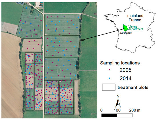
Figure 1.
Map of the sampling plots in 2005 and 2014 over 20 cm-color orthophotograph from the French National Institute of Geographic and Forest Information (IGN, 2017).

Table 1.
Experimental design of SOERE ACBB with the studied treatments. The vertical bold line indicates the date of sampling (March 2014); shaded zones indicate grassland phases.
Small blocks (0.4 ha) supported five treatments differentiated by fertilization and duration of grassland phase (Table 1): 3 years of fertilized ley (CGC), 6 years of N-fertilized ley (GGC) and 6 years ley (GGCN-) without nitrogen fertilization. As a control, there was one treatment with permanent cropland (CCC) and one other with permanent grassland (GGG). Treatments were replicated 4 times in 4 separated blocks. Grassland treatments in small blocks were all under mowing regime (4 cuts per year) with harvest exported. N-exports were replaced by mineral N fertilization in the form of NH4NO3. For mowed grasslands, multi-species mixtures were sown including Dactylis glomerata L. (cocksfoot) cultivar Ludac with a density of 12 kg ha−1, Festuca arundinacea Schreb (tall fescue) cultivar Soni with a density of 10 kg ha−1 and Lolium perenne L. (rye-grass) cultivar Milca with a density of 5 kg ha−1. Fertilization varied with years and ranged between 36 and 160 kg N ha−1 year−1 for cropland, and between 170 and 380 kg N ha−1 year−1 for fertilized grasslands. Unfertilized grassland received no N fertilization.
In big blocks (3 ha), permanent grasslands (GGG) and the temporary grasslands with crop rotations (GGCN+) were repeated in a similar condition, i.e., with mowing regime. In addition, two more grazing treatments were installed: one with permanent grassland managed as pasture (GGGp) and another with 6 years ley managed by grazing (GGCp). In these two treatments, a leguminous species in the multi-species mixture (Trifolium repens L. (white clover) cultivar Menna with a density of 2 kg ha−1) and dung return replaced mineral N fertilization (Table 1). Grazing intensity was 15 to 20 livestock unit per ha, from March to December with 20 to 50 days per year.
The cropping treatment established on small blocks as permanent cropland (CCC) with different periods of ley grassland (GGC and CGC) consisted of Zea mays L. (maize) cultivar Texxud sown at a density of 85,000 grains ha−1 followed by Triticum aestivum L. (wheat) cultivar Caphorn sown at density of 150 grains m−2 and 2006 Hordeum vulgare L. (barley) cultivar Vanessa sown at density of 165 grains m−2. All straw residues were exported. This scheme was repeated for the permanent cropland control (CCC).
Before the beginning of the experiment in 2005, total surface had been homogenized by 3 years of cropland (barley, maize and triticale).
2.2. Soil Sampling and Geostatistical Analyses
Before the installation of the treatments, in spring 2005, 400 cores (Ø 18 mm and 120-cm depth) were taken at the SOERE ACBB site with 350 located on small plots (Figure 1). Each core sample was subsequently cut to separate three depths: 0–30, 30–60 and 60–90 cm. The Poll campaign point was drawn randomly on a 10 × 10 grid principle. In addition, 76 samples were taken in triplicate at 50-cm distances to account for microscale variability. The soil samples were air-dried, sieved at 2 mm and grounded. In spring 2014, the sampling procedure was repeated at the same 400 georeferenced points complemented by 133 additional points to improve resolution (Figure 1).
Total carbon and total nitrogen concentrations ([C] and [N]) of soil samples were determined using an elementary analyzer (Flash EA, Thermo Electron Corporation, Bremen, Germany).
In spring 2005, the soil bulk density was determined for 27 soil profiles established in all treatments at the three depths: 0–30, 30–60 and 60–90 cm, whereas in 2014, a bulk density of 0–30 cm depth soil was measured in 112 points. For the 2005 data, we used the means per depth. For 2014 data, a mean of bulk density was calculated for each treatment with 2016 data after verifying that the data did not present a spatial residual structure (fit.gstatModel function of package gstat). As the bulk density values were not significantly different from the ones recorded for the same treatments in 2005, we did not make any correction for equivalent mass. This may be correct for our site, as it has been under similar management for 100 years. We did not expect significant bulk density changes on the decadal timescale of the experiment. For 30–60 and 60–90 cm 2014 data, we used the bulk density measurements of 2005. The soil bulk density (d; g cm−3) was the weight of the solid phase (Ms, dried soil at 105 °C) over the cylinder total volume (V) of sampled soil:
Soil C stocks (t ha−1) were calculated with Equation (2):
where [C] is the soil C concentration (mg g−1), p is with the depth of the layer (cm) and d is the soil bulk density (g cm−3; Equation (1)) [28].
The plots’ spatial patterns of carbon stock in 2005 and 2014 (C2005 stock and C2014 stock) were estimated using data from each sampling location coupled with a regression co-kriging method [29]. This approach combines a linear regression of carbon stocks on auxiliary variables with a co-kriging interpolation of the regression residuals. We used the treatment information as an auxiliary variable of C2005 stock and C2014 stock. We also computed the auto- and crossed variograms of the residuals (Table S1) and fitted a linear model of co-regionalization (LMCR). The coefficients of the linear model are then recomputed using the generalized ordinary least squared. The range of the LMCR was selected following a fitting procedure of the auto-variograms [30]. Variograms and models revealed spatial structure differences. Range as the distance at the stable semi-variance when the data have no correlation, nuggets representing error at small scale and partial sill representing increased semi-variance without nugget effects revealed small-scale variability. The whole procedure was validated using a leave-one-out cross-validation. We computed a standardized squared prediction error, where the mean should be equal to 1.0 and the median to 0.455 [31]. We then computed estimates of the carbon stock of the soil at the unsampled sites using universal co-kriging to produce a raster map of C2005 stock and C2014 stock. We implemented this procedure using the R package gstat [32].
The temporal changes of SOC stocks (kg ha−1 9 yrs−1) were estimated by calculating the difference between the raster maps of the 2005 and 2014 carbon stocks:
Evolution of C stocks per year based on initial stocks (C dynamic, ‰) was calculated as:
The C/N ratio was calculated with the raster maps for 2005 and 2004 C stocks and the nitrogen stocks as:
The variability was classified from the estimated data standard score (Z score) [33], calculated as:
as “0” is no change in carbon, with standard deviation (SD) calculated with variance (Var) and covariance (CoVar) [29]:
The Z score critical value corresponds to a p-value significance level, as for Z score > 1.96 or <−1.96, the p-value is 0.05 *; for Z score > 2.58 or <−2.58, the p-value is 0.01 ** and for Z score > 3.29 or <−3.29, the p-value is 0.001 *** [33].
All calculations and analyses were carried out with R (Studio Version 1.0.136). Treatment differences were analyzed by ANOVA followed by Tukey’s post hoc test (package agricolae).
2.3. Physicochemical Soil Analyses
To explain the spatial distribution of SOC stock changes, we analyzed pedological parameters of selected samples. In each of the 4 big plots, we chose 3 samples characterized by SOC gain and 3 samples characterized by SOC loss (except CGGp, where there are only SOC loss points). We performed additional analyses to characterize physicochemical parameters of these samples taken in 2014. Specific surface area (SSA, m2 g−1) is a property of soil defined as the total surface area per gram. It was shown to be correlated to water loss of air-dried samples [34]. Therefore, we estimated surface area as residual water loss from dried samples. Approximately 50 g of field moist soil was placed in tinfoil buckets and dried at 30 °C for 48–72 h before sieving at 2 mm. Thereafter, 10 g of a dried soil was put in an oven at 30 °C and 30% humidity until constant mass before determining the weight. Thereafter, the sample was dried at 105 °C to a constant mass and the weight (moven-dry in g) was recorded. Water loss was determined and the specific surface area (SSA, m2 g−1) was estimated after [34,35]:
The proportions of five classes of soils particles were determined according to standard NF X 31–107 (afnor 2003) including clays (<2 μm), fine silt (2 to 20 μm), coarse silt (20 to 50 μm), fine sand (0.050 to 0.200 mm) and coarse sand (0.2 to 2.0 mm). Separation of particle size classes was carried out after destruction of organic matter by hydrogen peroxide (H2O2). The sand fractions were separated by wet sieving. The fractions <50 μm were determined by the pipette method after sedimentation. The results were expressed relative to the mineral phase (sum of 5 fractions = 1000).
Fe, Al and Si oxides (Feo, Alo and Sio) were determined with the method described by [36]. Briefly, 1.25 g of grounded soil was agitated for 4 h in the dark at 20 °C with 50 mL of ammonium oxalate (0.1134 mol L−1) and oxalic acid (0.0866 mol L−1) solution at pH 3. Total amounts of Fe, Al and Si were determined by using the dithionite–citrate–bicarbonate (DCB) extraction method [37]. Briefly, 0.5 g of grounded soil was extracted at 80 °C with 25 mL 0.03 M sodium-citrate dithionite (0.267 mol L−1). Thereafter, 1.5 mL of reductive solution of sodium dithionite (200 g L−1) was added and the solution was stirred for 30 min. Inductively coupled plasma atomic emission spectroscopy (ICP-AES) analyses were performed on the filtered extracts for Feo, Alo and Sio and Fe, Al and Si.
Soil resistivity was expressed in Ω m−1 and represented its capacity to limit the passage of an electric current. Multi-electrode devices make it possible to describe the lateral and vertical variations of electrical resistivity by means of quasi-continuous probes and electric tows. The multipole Automatic Resistivity Profiling (ARP©) was composed at the head of a dipole emitter of electric current followed by a series of three dipole receivers for measuring the electric soil potential. The spacing of each dipole increased with distance from the transmitter dipole and it was 0.5, 1 and 2 m for the first, second and third dipoles, respectively (their depth of investigation was approximately equal to their spacing). The electrical current used for injection was 10 mA. The system makes it possible to carry out resistivity measurements at a pitch of 20 cm, whatever the speed of advancement. The location of measurements was provided by a Trimble Ag114 GPS with a subscription to differential corrections (Thalès-Omnistar) with a positioning accuracy of 1 m minimum.
All calculations and analyses were carried out with R (Studio Version 1.0.136). A two-way ANOVA statistical analysis followed by Tukey’s honest significant difference (HSD) post-hoc test (package agricola) allowed us to evaluate differences in physicochemical analyses between agricultural treatments and by areas with SOC gains and loss.
In order to identify explanatory factors for we carried out a principal component analysis (PCA) (package FactoMineR). The PCA function of the FactoMineR package automatically transformed data to a standardized normal distribution. The number of observations was 24 and the number of biophysical variables used for PCA was 10 [38].
3. Results
3.1. SOC Concentrations and Bulk Density
Soil organic carbon concentrations varied between 7.6 and 16.9 mg g−1 in 2005 and between 7.9 and 19.1 mg g−1 in 2014 in the first 30 cm of soil (Table 2). At lower depths, SOC concentrations were 10 times lower. The SOC concentrations at all depths were similar in 2005 and 2014. In the topsoil, the bulk density varied between 1.26 and 1.47 g cm−3 in 2005 and 1.40 and 1.65 g cm−3 in 2014. Although the bulk density tended to have higher values in 2014, these differences were not significant.
Table 2.
Variability of carbon and nitrogen concentrations and bulk density for the whole site in the two sampling years.
3.2. SOC Stocks and Spatial Patterns
In 2005, predicted SOC stocks ranged between 13.9 and 62.2 t ha−1 (Table 3). They decreased strongly with soil depth. The data show a spatial gradient of SOC stocks at 0–30 cm depth, with the highest values recorded for big plots and the lowest for small plots, especially in the western part of the site. In 2014, this variability seems to be reduced and was related to the grassland management treatment.
Table 3.
Predicted carbon stocks and their evolution under different grassland management. SD is standard deviation, * is statistical significances of storage’s Z-score (shown in Figure 3, * p-value is <0.05, ** p-value is <0.01 and *** p-value is <0.001) and a lowercase letter is statistical significance from ANOVA and Tukey’s HSD post-hoc test. Total stock changes over 9 years (ΔC) are printed in bold.
In deep soil (30–60 and 60–90 cm depth), the strong small-scale heterogeneity indicated by high nugget effects is randomly represented instead and not spatially organized in either treatment in 2014 (Figure 2).
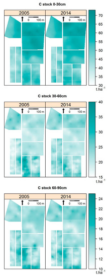
Figure 2.
Co-kriging predicted C2005 stock and C2014 stock for 0–30, 30–60 and 60–90 cm depths.
The SOC stock changes in 9 years under different grassland management techniques derived from subtraction of predicted SOC stocks at all three depths are shown in Figure 3a and for the whole profile in Figure 3b. As expected in topsoil (0–30 cm), continuous grassland (GGG) increased SOC storage by 4.9 t ha−1 and continuous cropland (CCC) reduced it by 3.3 t ha−1 over the 9 years (Table 3). Apart from temporarily grazed grassland GGCp, which lost SOC (−4.3 t ha−1 in 9 years), all other ley grasslands showed no significant changes in SOC stocks (Table 3 and Figure 3). In deep soil (30–60 and 60–90 cm), the variation in SOC storage was low and not significantly different from zero, except for the treatments CGC and GGG, which showed C loss in 60–90 cm (−0.8 and −0.9 t ha−1 in 9 years, respectively) (Table 3 and Figure 3). For whole profiles, our data showed an increase in SOC storage for GGG and a decrease from CCC (Table 4). It was interesting to note that especially in small blocks under ley grassland and big blocks, we could observe areas with carbon loss and gain regardless of their general trends (loss, gain or no change; Figure 3).
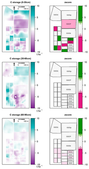
Figure 3.
Soil organic carbon (SOC) storage change calculated by different co-kriging-predicted C2005 stock and C2014 stock in for 0–30, 30–60 and 60–90 cm depths. Z-score calculated for each treatment (for Z-score > 1.96 or <−1.96, the p-value is 0.05 *, for Z-score > 2.58 or <−2.58, the p-value is 0.01 ** and for Z-score > 3.29 or <−3.29, the p-value is 0.001 ***).
Table 4.
Predicted carbon stocks and their evolution in the whole soil profiles under different grassland management. SD is standard deviation, * is statistical significances of storage’s Z-score (shown in Figure 3, * p-value is <0.05, ** p-value is < 0.01) and a lowercase letter is statistical significance from ANOVA and Tukey’s HSD post-hoc test. Total stock changes over 9 years (ΔC) are printed in bold.
The variograms and cross-variograms of SOC are plotted in Figure 4. In all variograms, the average of semi-variogram values was represented over a distance interval of 7 m and the model type was exponential with nuggets.
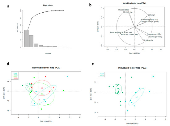
Figure 4.
Principal component analysis for pedological soil parameters. a Eigenvalues of principal components; b Variable factor map; c Individual factor map belong to treatment; and d Individual factor map belong to gain and loss C dynamic.
3.3. Pedological Soil Parameters in 3-ha Plots Showing Contrasted Response (SOC Gain or Loss) to Similar Treatment
As the SOC stock changes in the 3-ha plots showed contrasting responses despite similar soil management, we analyzed pedological soil parameters in zones with SOC gain and SOC loss in the four treatments. Soil texture separated in five fractions did not show significant differences among treatments, except for coarse sand (200–2000 µm) varying from 62.8 g kg−1 for GGCp to 99.7 g kg−1 for GGGp (Table 5). However, soils sampled in areas with SOC gain and/or loss showed contrasting soil texture, which was not influenced by the experimental treatments. Sampling plots with SOC gain were characterized by higher coarse sand fraction with 102.8 g kg−1 as compared to 72.3 g kg−1 in sampling plots with SOC loss (Table 5). In addition, lower fine and coarse silt content was found for SOC gain sampling plots as compared to sampling plots showing SOC loss, while no differences were found for soil clay content (Table 5).
Table 5.
Pedologic soil parameter measured for selected points (2014) in big plots (a) and predicted data for these points (b). Lowercase letter is statistical significance of the two-way ANOVA and Tukey’s HSD test: a, b and c for management treatments and a’ and b’ for C gain or loss points, respectively.
Big plot soils of all three treatments presented similar Fe, Al and Si oxide concentrations (Table 5 and Table 6). Significant differences for sampling plots with SOC gain and loss were recorded for amorphous and crystalline Al oxides and crystalline Fe oxides, which were higher in samples showing SOC gain as compared to sampling plots characterized by SOC loss (Table 5 and Table 6). Soil specific surface area as estimated by water loss from dry samples comprised between 35.48 and 36.78 m2 g−1, without any significant differences between treatments or sampling plots characterized by SOC gain and loss. Soil resistivity ranged between 79.3 at 134.5 Ω m−1 and was significantly higher for GGCb than all other treatments (Table 5 and Table 6).
Table 6.
Predicted SOC for the points, where pedological parameters (Table 5) were measured. Lowercase letter is statistical significance of the two-way ANOVA and Tukey’s HSD post-hoc test: a, b and c for management treatments and a’ and b’ for C gain or loss points, respectively.
The Pearson correlation showed that the C dynamic was negatively correlated to initial C and N stocks (r = −0.57 and −0.58, respectively, p-value < 0.01) and fine silt (r = −0.44, p-value < 0.05) and positively correlated to coarse sand (r = 0.61, p-value < 0.01) (Figure 4b). Both parameters were negatively correlated (r < −0.68, p-value < 0.001) to Al and Fe soil concentrations, which strongly correlated (r = 0.98, p-value < 0.001) (Figure 4b). SSA was correlated to Al and Fe (r = 0.78, p-value < 0.001) and also negatively to fine and coarse silt (r = −0.76 and −0.74, respectively, p-value < 0.001).
The first two components explained 78.8% of the total variance. The first dimension (46.9%) was correlated positively to the Fe (r = 0.87), Al (r = 0.85), C dynamics (r = 0.75), SSA (r = 0.71), N dynamic (r = 0.71) and C/N change (r = 0.45), while it was negatively correlated to fine and coarse silt (r = −0.79 and −0.74, respectively) (Figure 4b). The second dimension (31.8%) was correlated positively to the C2005 stock (r = 0.88), N2005 stock (r = 0.85) and SSA (r = 0.59), while it was negatively correlated to C/N change (r = −0.69) and C dynamics (r = −0.50) (Figure 4b).
4. Discussion
4.1. Grassland Management Effects on SOC Storage
4.1.1. Cropland Versus Grassland
Our data indicated significant SOC stock changes after 9 years of treatment only for two treatments on 0.4-ha blocks, permanent cropland (CCC) and permanent mowed grassland (GGG). While cropland lost −7.5‰ of 0–30 cm soil stock each year, grassland showed a SOC stock increase of 11.7‰, representing +0.54 tC ha−1 y−1 for mowed grassland stock, close to former estimations for French grasslands of +0.5 tC ha−1 y−1 [39].. These data are in agreement with the net ecosystem exchange determined by Eddy flux tower measurements for the same treatments [40] (Senapati et al., 2014). The gains in grassland soil were higher than those reported by [41], who reported an average SOC stock increase of +0.34 tC ha−1 y−1 after grassland establishment from compiled literature data. In cropland soil, C loss was −0.36 tC ha−1 y−1, which was approximately three times lower as compared to the data for French soils reported by [39]. Lal and Bruce indicated highly variable SOC loss across the world’s cropland soils, ranging between −0.2 and −12‰ per year, with a world average of −0.6‰ [42]. These differences may be explained by contrasting pedoclimatic conditions and contrasting agricultural management practices [9,43]. Globally, agriculture has induced, since its beginning, a SOC loss of 116 Gt [5]. Rebuilding these SOC stocks could increase soil fertility and climate resilience [44]. That is why the introduction of ley grassland into cropping systems was promoted [10]. However, generally, SOC stocks can decrease more rapidly than they can increase [20,39]. Therefore, grassland duration should probably exceed the duration of crop phases. At our site with loamy agricultural soil and productive mowed grasslands, which had been under agricultural use for at least 100 years, SOC seemed to increase at least as rapidly as it was lost. Consequently, all temporary grasslands, which had been under cropland for the last three years, maintained their C stocks.
The magnitude of SOC loss and gain may be strongly dependent on the site history and how far SOC is away from equilibrium. Our results suggest that agricultural use already depleted SOC to a large extent and that SOC gain could be as fast as its loss, a precondition for the benefit of introduction of ley grassland into the cropping cycle as a promising strategy to maintain and build up SOC stocks. In the following, we discuss how these processes may be influenced by contrasting grassland management strategies.
4.1.2. Management of Temporary Grassland
Temporary fertilized grassland of 6 years showed slight increases in initial C stock of 1.7‰ in 0–30 cm soil, whereas shorter duration and absence of fertilization tended to decrease SOC and N stocks. The impact of N fertilization on SOC storage was recognized in several studies [7,9,16,20,45]). However, a meta-analysis conducted by [46] revealed that even if N addition increased C input by higher plant biomass production, it did not affect SOC storage in grassland soil. This may be explained by higher investment in aboveground biomass production leading to reduced belowground SOC storage [47]. Moreover, SOC storage changes upon N fertilization may be related to changes in the biogeochemical composition of root material [48]. The contrasting SOC stock responses to fertilization may be related to strong variability of ecosystems’ response to management and can be due to increased C mineralization rates following fresh organic matter supply in grassland soils [16]. To achieve long term benefits in terms of ecosystem services derived from SOC, fertilization and a minimum duration of mowed temporary grassland phase between 3 and 6 years was suggested [10,16]. In mowed temporary grasslands, SOC stock changes were not significantly different from 0, despite differences in terms of duration and fertilization. Thus, mowed temporary grasslands were able to maintain SOC stocks of croplands at a decadal timescale regardless of their management.
The impact of grazing as compared to mowing on SOC stock changes was studied on 3-ha blocks, with space necessary for pasture implementation. Six-year temporary grassland managed by grazing showed, surprisingly, the highest decrease in C stock in the first 30 cm with −4.3 t ha−1 in 9 years, which is more than what was recorded for permanent cropland. Interestingly, the net ecosystem exchange determined by Eddy flux tower measurements did not confirm this trend (data not shown). This could indicate that the CO2 uptake observed by these measurements does not accumulate in the soil pool under this treatment. The mowed temporary grassland, on the other hand, maintained SOC stocks. This might be explained by biogeochemical processes involving soil organic matter (SOM) and microorganisms, which were shown to be different under grazing and mowing [24] and which may have induced SOC losses after replacement of the grazed temporary grassland by three years of crop. Another possible explanation may be related to soil-inherent properties.
4.2. The Importance of Scale for Assessing Management Effects on SOC Storage
In view of our results, it seems to be important to consider the scale of observation. Carbon stocks may vary in space but also along the profile [49,50] and the choice of scale may, thus, affect the results and management decisions. For example, analysis of samples taken at 0–10-cm depth indicated that absence of N fertilization leads to decreasing SOC stocks [16], while in the present study, with samples taken at 0–30 cm, there was no measurable effect of N fertilization on SOC stocks. Moreover, significant effects recorded at 0–30 cm may no longer be visible taking into consideration SOC stocks in the whole soil profile (0–90 cm). The impact of depth on SOC storage and SOM dynamics has been recognized by many authors e.g., [51,52]. While it is generally accepted that plant carbon input into deep soil layers occurs much more slowly than in topsoil [53], recent studies indicate that SOC stored at depth may be responsive to management despite its apparent long residence times [54,55]. Our data indicate that in temperate loamy soil under grassland, SOC stored in layers below 30 cm of depth was barely responsive to management changes at decadal time scale.
At the landscape scale, our results are somewhat contrasting from those recorded at the plot scale, with 3-ha blocks showing a contrasting response to management as compared to 0.4-ha blocks, with areas characterized by positive and negative SOC storage. Therefore, average SOC storage and dynamics were less clear than for similar treatments in 0.4-ha blocks. For example, permanent grasslands under mowing treatment did not show a significant SOC stock increase after 9 years of treatment in 3-ha blocks, while positive changes were significant in 0.4-ha blocks. This may be due to the fact that factors controlling SOC at the plot scale are less important than at the landscape scale [26,56]. Spatial differences of SOC changes have been observed before and were found to reflect both topography and geological pattern [57]. While in this 23-ha experiment, climate, topography and vegetation may be excluded as controlling factors for contrasting SOC stock changes at the two different spatial scales, we found that differences in soil properties separated sampling points with SOC gain and loss (Figure 4). Our data indicate that it is important to consider soil mineralogical properties. These may be related to soil type, parent material and weathering intensity [58,59], which were found to explain SOC stocks at national or subnational scales [60,61], particularly for subsoil [59], and may interfere with management effects [62,63],. In particular, the soil moisture regime was indicated as an important controlling factor, which may directly affect soils’ potentials to store SOC [56]. It is interesting to note that in our study, at a 23-ha site, plots with contrasting SOC changes also showed differences in soil parameters. We suggest that the spatially heterogeneous nature of the mineral soil may be most likely related to the parent material and the complex hydrology of the soil, which is characterized by numerous preferential flow pathways [25], which may have influenced weathering processes. In line with authors working at the landscape scale, we therefore suggest that soil properties should be taken into account at all scales when evaluating SOC responses to management practices.
5. Conclusions
We investigated ley grassland management effects on SOC stock changes during a 9-year field experiment in temperate loamy soil at two different scales using a geostatistical sampling approach. Our data indicated SOC increases under continuous grasslands and SOC decreases under continuous agriculture. Introduction of mowed grassland during cropping maintained SOC regardless of its management. When analyzing bigger scales, the results were different, as zones with carbon gains and losses occurred in most treatments. These contrasting trends within the same treatment were related to soil characteristics. Grazing of ley grassland could reduce SOC stocks and show, at the same time, CO2 uptake, indicating that this additional C may contribute to other pools than SOC. We conclude that even for the same soil type, local variability in soil characteristics influences SOC stock responses to management. For a detailed assessment of C fluxes, ground-based evaluation of stock changes in different pools is necessary.
Supplementary Materials
The following are available online at https://www.mdpi.com/2073-4395/10/12/2016/s1, Table S1: Variogram (2005, 2014) and cross-variogram (2005 × 2014) model coefficients (nugget, partial sill and range) and cross validation mean.
Author Contributions
A.C. (Alexandra Crème) and C.R. designed the experiment. A.C. (Alexandra Crème) carried out the work and wrote the manuscript. N.P.A.S. helped with the statistical exploitation of the data. M.-L.D. was responsible for the field experiment. S.L.M. helped with the data curation. E.V. helped with data curation and resources. A.C. (Abad Chabbi) helped with the funding acquisition, investigation and supervision. All authors contributed to the interpretation of the data and the writing of the manuscript. All authors have read and agreed to the published version of the manuscript.
Funding
We acknowledge funding from the funding organisms of SOERE structures INRA, CNRS, ALLENVI, ANR, European commission. We also acknowledge ADEME for the funding of the AEGES project.
Acknowledgments
We acknowledge funding from the funding organisms of SOERE structures INRA, CNRS, ALLENVI, ANR, European commission. We also acknowledge ADEME for the funding of the AEGES project. We thank the technical staff of UE Ferlus, Lusignan.
Conflicts of Interest
The authors do not have any conflict of interest.
References
- Batjes, N.H. Total carbon and nitrogen in the soils of the world. Eur. J. Soil Sci. 2014, 65, 10–21. [Google Scholar] [CrossRef]
- IPCC. Fifth Assessment Report WG1; IPCC: Geneva, Switzerland, 2013. [Google Scholar]
- Smith, P. Soil carbon sequestration and biochar as negative emission technologies. Glo. Chang. Biol. 2016, 22, 1315–1324. [Google Scholar] [CrossRef] [PubMed]
- Chabbi, A.; Lehmann, J.; Ciais, P.; Loescher, H.W.; Cotrufo, M.F.; Don, A.; SanClements, M.; Schipper, L.; Six, J.; Smith, P.; et al. Aligning agriculture and climate policy. Nat. Clim. Chang. 2017, 7, 307–309. [Google Scholar] [CrossRef]
- Sanderman, J.; Heng, T.; Fiske, G.J. Soil carbon debt of 12,000 years of human land use. Proc. National Acad. Sci. 2017, 114, 9575–9580. [Google Scholar] [CrossRef]
- FAO. 2016. Available online: www.fao.org/climate-change (accessed on 23 January 2020).
- Lal, R. Soil Carbon Sequestration Impacts on Global Climate Change and Food Security. Science 2004, 304, 1623–1627. [Google Scholar] [CrossRef]
- Paustian, K.; Lehmann, J.; Ogle, S.; Reay, D.; Robertson, G.P.; Smith, P. Climate-smart soils. Nat. Cell Biol. 2016, 532, 49–57. [Google Scholar] [CrossRef]
- Conant, R.T.; Paustian, K.; Elliott, E.T. Grassland Management and Conversion into Grassland: Effects on Soil Carbon. Ecol. Appl. 2001, 11, 343–355. [Google Scholar] [CrossRef]
- Lemaire, G.; Gastal, F.; Franzluebbers, A.; Chabbi, A. Grassland–Cropping Rotations: An Avenue for Agricultural Diversification to Reconcile High Production with Environmental Quality. Environ. Manag. 2015, 56, 1065–1077. [Google Scholar] [CrossRef]
- Stahl, C.; Fontaine, S.; Klumpp, K.; Picon-Cochard, C.; Grise, M.M.; Dezécache, C.; Ponchant, L.; Freycon, V.; Blanc, L.; Bonal, D.; et al. Continuous soil carbon storage of old permanent pastures in Amazonia. Glob. Chang. Biol. 2017, 23, 3382–3392. [Google Scholar] [CrossRef]
- Scurlock, J.M.O.; Johnson, K.; Olson, R.J. Estimating net primary productivity from grassland biomass dynamics measurements. Glob. Chang. Biol. 2002, 8, 736–753. [Google Scholar] [CrossRef]
- Rumpel, C.; Crème, A.; Ngo, P.; Velásquez, G.; Mora, M.; Chabbi, A. The impact of grassland management on biogeochemical cycles involving carbon, nitrogen and phosphorus. J. Soil Sci. Plant Nutr. 2015, 15, 353–371. [Google Scholar] [CrossRef]
- European Commission. CAP Explained: Direct Payments for Farmers 2015–2020; Publications Office of the EU: Luxembourg, 2017. [Google Scholar]
- Acharya, B.S.; Rasmussen, J.; Eriksen, J. Grassland carbon sequestration and emissions following cultivation in a mixed crop rotation. Agric. Ecosyst. Environ. 2012, 153, 33–39. [Google Scholar] [CrossRef]
- Crème, A.; Rumpel, C.; Le Roux, X.; Romian, A.; Lan, T.; Chabbi, A. Fertilised ley grassland has a legacy effect on soil organic matter quantity and quality and microbial activities favourable to C sequestration. Soil Biol. Biochem. 2018, 122, 203–210. [Google Scholar] [CrossRef]
- Richardson, A.E.; Kirkby, C.A.; Banerjee, S.; Kirkegaard, J.A. The inorganic nutrient cost of building soil carbon. Carbon Manag. 2014, 5, 265–268. [Google Scholar] [CrossRef]
- Van Groenigen, J.W.; Van Kessel, C.; Hungate, B.; Oenema, O.; Powlson, D.S.; Van Groenigen, K.J. Sequestering Soil Organic Carbon: A Nitrogen Dilemma. Environ. Sci. Technol. 2017, 51, 4738–4739. [Google Scholar] [CrossRef] [PubMed]
- Kirkby, C.; Richardson, A.E.; Wade, L.J.; Passioura, J.B.; Batten, G.D.; Blanchard, C.; Kirkegaard, J.A. Nutrient availability limits carbon sequestration in arable soils. Soil Biol. Biochem. 2014, 68, 402–409. [Google Scholar] [CrossRef]
- Schipper, L.A.; Parfitt, R.; Fraser, S.; Littler, R.; Baisden, W.; Ross, C.W. Soil order and grazing management effects on changes in soil C and N in New Zealand pastures. Agric. Ecosyst. Environ. 2014, 184, 67–75. [Google Scholar] [CrossRef]
- INRA. Quelle Contribution de l’agriculture Française à la Réduction des Émissions de Gaz à Effet de Serre? INRA: Paris, France, 2013. [Google Scholar]
- McSherry, M.E.; Jackson, M.L. Iron oxide removal from soils and clays by a dithionite–citrate system buffered with sodium bicarbonate. In Clays and Clay Minerals: Proceedings of the Seventh National Conference; Elsevier: Amsterdam, The Netherlands, 1960; pp. 317–327. [Google Scholar]
- Klumpp, K.; Fontaine, S.; Attard, E.; Le Roux, X.; Gleixner, G.; Soussana, J.-F. Grazing triggers soil carbon loss by altering plant roots and their control on soil microbial community. J. Ecol. 2009, 97, 876–885. [Google Scholar] [CrossRef]
- Gilmullina, A.; Rumpel, C.; Blagodatskaya, E.; Chabbi, A. Management of grasslands by mowing versus grazing—Impacts on soil organic matter quality and microbial functioning. Appl. Soil Ecol. 2020, 156, 103701. [Google Scholar] [CrossRef]
- Chabbi, A.; Kögel-Knabner, I.; Rumpel, C. Stabilised carbon in subsoil horizons is located in spatially distinct parts of the soil profile. Soil Biol. Biochem. 2009, 41, 256–261. [Google Scholar] [CrossRef]
- Moni, C.; Chabbi, A.; Nunan, N.; Rumpel, C.; Chenu, C. Spatial dependance of organic carbon–metal relationships: A multi-scale statistical analysis, from horizon to field. Geoderma 2010, 158, 120–127. [Google Scholar] [CrossRef]
- Senapati, N.; Chabbi, A.; Smith, P. Modelling daily to seasonal carbon fluxes and annual net ecosystem carbon balance of cereal grain-cropland using DailyDayCent: A model data comparison. Agric. Ecosyst. Environ. 2018, 252, 159–177. [Google Scholar] [CrossRef]
- Mathieu, C.; Pieltain, F. Analyse Physique des Sols: Méthodes Choisies; Tec & Doc Lavoisier: Washington, DC, USA, 1998. [Google Scholar]
- Pebesma, E.; Duin, R.N.M.; Burrough, P.A. Mapping sea bird densities over the North Sea: Spatially aggregated estimates and temporal changes. Environmetrics 2005, 16, 573–587. [Google Scholar] [CrossRef]
- Orton, T.; Pringle, M.; Page, K.L.; Dalal, R.C.; Bishop, T. Spatial prediction of soil organic carbon stock using a linear model of coregionalisation. Geoderma 2014, 230–231, 119–130. [Google Scholar] [CrossRef]
- Webster, R.; Oliver, M.A. Geostatistics for Environmental Scientists, 2nd ed.; John Wiley & Sons: Hoboken, NJ, USA, 2007. [Google Scholar]
- Pebesma, E. Multivariable geostatistics in S: The gstat package. Comput. Geosci. 2004, 30, 683–691. [Google Scholar] [CrossRef]
- Kreyszig, E. Solution Manual 9th Edition Advanced Engineering; 2011; ISBN 978-0-470-91361-1. Available online: https://www.google.com.hk/url?sa=t&rct=j&q=&esrc=s&source=web&cd=&ved=2ahUKEwjX3svDmt7tAhVFfd4KHVjXDE0QFjABegQIBBAC&url=http%3A%2F%2Fwww.icivil-hu.com%2FCivil-team%2F2nd%2FApplied%2Fsolution_manual_of_advanced_engineering_mathematics_by_erwin_kreyszig_9th_edition.pdf&usg=AOvVaw0RHZswAyar7Zh81zMjlwNn (accessed on 21 December 2020).
- Parfitt, R.L.; Whitton, J.S.; Theng, B.K.G. Surface reactivity of a horizons towards polar compounds estimated from water adsorption and water content. Soil Res. 2001, 39, 1105. [Google Scholar] [CrossRef]
- Theng, B.K.G.; Ristori, G.G.; Santi, C.A.; Percival, H.J. An improved method for determining the specific surface areas of topsoils with varied organic matter content, texture and clay mineral composition. Eur. J. Soil Sci. 1999, 50, 309–316. [Google Scholar] [CrossRef]
- Tamm, O. Eine Methode zur Bestim mung der anorganischen Komponenten des Gelkomplexes im Boden. Meddel Statens Skogsforsoksanst 1922, 19, 385–404. [Google Scholar]
- Mehra, O.P. Iron Oxide Removal from Soils and Clays by a Dithionite-Citrate System Buffered with Sodium Bicarbonate. Clays Clay Miner. 1958, 7, 317–327. [Google Scholar] [CrossRef]
- Gauch, H.G. Multivariate Analysis in Community Ecology; Cambridge University Press: Cambridge, UK, 1982. [Google Scholar]
- Arrouays, D.; Balesdent, J.; Germon, J.C.; Jayet, P.A.; Soussana, J.F.; Stengel, P. Increasing Carbon Stocks in French Agricultural Soils? INRA: Paris, France, 2002. [Google Scholar]
- Senapati, N.; Chabbi, A.; Gastal, F.; Smith, P.; Mascher, N.; Loubet, B.; Cellier, P.; Naisse, C. Net carbon storage measured in a mowed and grazed temperate sown grassland shows potential for carbon sequestration under grazed system. Carbon Manag. 2014, 5, 131–144. [Google Scholar] [CrossRef]
- Post, W.M.; Kwon, K.C. Soil carbon sequestration and land-use change: Processes and potential. Glob. Chang. Biol. 2000, 6, 317–327. [Google Scholar] [CrossRef]
- Lal, R.; Bruce, J. The potential of world cropland soils to sequester C and mitigate the greenhouse effect. Environ. Sci. Policy 1999, 2, 177–185. [Google Scholar] [CrossRef]
- Ogle, S.M.; Breidt, F.J.; Paustian, K. Agricultural management impacts on soil organic carbon storage under moist and dry climatic conditions of temperate and tropical regions. Biogeochemistry 2005, 72, 87–121. [Google Scholar] [CrossRef]
- Rumpel, C.; Amiraslani, F.; Koutika, L.-S.; Smith, P.; Whitehead, D.; Wollenberg, E. Put more carbon in soils to meet Paris climate pledges. Nat. Cell Biol. 2018, 564, 32–34. [Google Scholar] [CrossRef] [PubMed]
- He, N.; Yu, Q.; Wang, R.; Zhang, Y.; Gao, Y.; Yu, G. Enhancement of Carbon Sequestration in Soil in the Temperature Grasslands of Northern China by Addition of Nitrogen and Phosphorus. PLoS ONE 2013, 8, e77241. [Google Scholar] [CrossRef] [PubMed]
- Lu, M.; Zhou, X.; Luo, Y.; Yang, Y.; Fang, C.; Chen, J.; Li, B. Minor stimulation of soil carbon storage by nitrogen addition: A meta-analysis. Agric. Ecosyst. Environ. 2011, 140, 234–244. [Google Scholar] [CrossRef]
- Sochorová, L.; Jansa, J.; Verbruggen, E.; Hejcman, M.; Schellberg, J.; Kiers, E.T.; Johnson, N.C. Long-term agricultural management maximizing hay production can significantly reduce belowground C storage. Agric. Ecosyst. Environ. 2016, 220, 104–114. [Google Scholar] [CrossRef]
- Poeplau, C.; Zopf, D.; Greiner, B.; Geerts, R.; Korvaar, H.; Thumm, U.; Don, A.; Heidkamp, A.; Flessa, H. Why does mineral fertilization increase soil carbon stocks in temperate grasslands? Agric. Ecosyst. Environ. 2018, 265, 144–155. [Google Scholar] [CrossRef]
- Bergstrom, D.W.; Monreal, C.M.; Jacques, E.S. Spatial dependence of soil organic carbon mass and its relationship to soil series and topography. Can. J. Soil Sci. 2001, 81, 53–62. [Google Scholar] [CrossRef]
- VandenBygaart, A.J.; Angers, D.A. Towards accurate measurements of soil organic carbon stock change in agroecosystems. Can. J. Soil Sci. 2006, 86, 465–471. [Google Scholar] [CrossRef]
- Lorenz, K.; Lal, R. The Depth Distribution of Soil Organic Carbon in Relation to Land Use and Management and the Potential of Carbon Sequestration in Subsoil Horizons. Adv. Agron. 2005, 88, 35–66. [Google Scholar] [CrossRef]
- Rumpel, C.; Kögel-Knabner, I. Deep soil organic matter—A key but poorly understood component of terrestrial C cycle. Plant. Soil 2011, 338, 143–158. [Google Scholar] [CrossRef]
- Balesdent, J.; Basile-Doelsch, I.; Chadoeuf, J.; Cornu, S.; Derrien, D.; Fekiacova, Z.; Hatté, C. Atmosphere-soil carbon transfer as a function of soil depth. Nat. Cell Biol. 2018, 559, 599–602. [Google Scholar] [CrossRef] [PubMed]
- Börjesson, G.; Bolinder, M.A.; Kirchmann, H.; Kätterer, T. Organic carbon stocks in topsoil and subsoil in long-term ley and cereal monoculture rotations. Biol. Fertil. Soils 2018, 54, 549–558. [Google Scholar] [CrossRef]
- Strey, S.; Boy, J.; Strey, R.; Weber, O.; Guggenberger, G. Response of soil organic carbon to land-use change in central Brazil: A large-scale comparison of Ferralsols and Acrisols. Plant. Soil 2016, 408, 327–342. [Google Scholar] [CrossRef]
- Wiesmeier, M.; Urbanski, L.; Hobley, E.; Lang, B.; Von Lützow, M.; Marin-Spiotta, E.; Van Wesemael, B.; Rabot, E.; Ließ, M.; Garcia-Franco, N.; et al. Soil organic carbon storage as a key function of soils—A review of drivers and indicators at various scales. Geoderma 2019, 333, 149–162. [Google Scholar] [CrossRef]
- Zhang, C.; McGrath, D. Geostatistical and GIS analyses on soil organic carbon concentrations in grassland of southeastern Ireland from two different periods. Geoderma 2004, 119, 261–275. [Google Scholar] [CrossRef]
- Percival, H.J.; Parfitt, R.L.; Scott, N.A. Factors controlling soil carbon levels in New Zealand grasslands: Is clay content important? Soil Sci. Soc. Am. J. 2000, 64, 1623–1630. [Google Scholar] [CrossRef]
- Chen, S.; Martin, M.P.; Saby, N.P.A.; Walter, C.; Angers, D.A.; Arrouays, D. Fine resolution map of top- and subsoil carbon sequestration potential in France. Sci. Total. Environ. 2018, 630, 389–400. [Google Scholar] [CrossRef]
- Chaplot, V.; Bouahom, B.; Valentin, C. Soil organic carbon stocks in Laos: Spatial variations and controlling factors. Glob. Chang. Biol. 2010, 16, 1380–1393. [Google Scholar] [CrossRef]
- Wiesmeier, M.; Barthold, F.; Spörlein, P.; Geuss, U.; Hangen, E.; Reischl, A.; Schilling, B.; Angst, G.; van Lützow, M.; Kögel-Knabner, I. Estimation of total organic carbon storage and its driving factors in soils of Bavaria (southeast Germany). Geoderma Reg. 2014, 1, 67–78. [Google Scholar] [CrossRef]
- Mayes, M.; Marin-Spiotta, E.; Szymanski, L.; Erdoğan, M.A.; Ozdoğan, M.; Clayton, M. Soil type mediates effects of land use on soil carbon and nitrogen in the Konya Basin, Turkey. Geoderma 2014, 232–234, 517–527. [Google Scholar] [CrossRef]
- Wiesmeier, M.; Von Lützow, M.; Spörlein, P.; Geuß, U.; Hangen, E.; Reischl, A.; Schilling, B.; Kögel-Knabner, I. Land use effects on organic carbon storage in soils of Bavaria: The importance of soil types. Soil Tillage Res. 2015, 146, 296–302. [Google Scholar] [CrossRef]


Publisher’s Note: MDPI stays neutral with regard to jurisdictional claims in published maps and institutional affiliations. |
© 2020 by the authors. Licensee MDPI, Basel, Switzerland. This article is an open access article distributed under the terms and conditions of the Creative Commons Attribution (CC BY) license (http://creativecommons.org/licenses/by/4.0/).