1. Introduction
Powdery mildew is considered a major fungal disease for grapevine worldwide. It is caused by the fungus
Erysiphe necator, an obligate biotrophic pathogen that produces significant damage to the crop including loss of yield and depreciation of the quality of wine or grapes [
1]. This disease manifests as a thin layer of grayish powdery appearance on the surface of both berries and leaves. This powder is caused by the mycelium of the fungus and conidia on the surface of the plant [
2]. The susceptibility of the vines to suffering from powdery mildew depends both on the sensitivity of the cultivar to this disease and the climatic conditions of the region where it is grown. Warm and wet climates favor the occurrence of this fungal disease [
3], which is able to affect any green organ of the plant (shoots, leaves and berries) [
4]. The initial infection occurs in isolated foci, and is barely perceptible visually, hampering the identification of powdery mildew infection at an early stage [
5]. Therefore, traditionally, the identification of this disease is based on visible signs of a pathogen once the plant has already been infected [
6]. Within this context, there is a clear need for techniques that allow the objective detection of the disease to achieve a standardized method for powdery mildew diagnosis in grapevine [
6] enabling an effective management of the vineyard in subsequent seasons. According to [
7] the correct monitoring of powdery mildew reduces the risk of disease appearance in following campaigns.
In recent years, optical sensor technologies have proven their efficiency in the evaluation of quality and safety in crops and agricultural materials [
8] by allowing samples to be inspected fast and non-destructively. Among those, hyperspectral imaging (HSI) stands out as one of the most promising techniques for the detection of plant diseases [
9], since it is not only capable of detecting and quantifying diseases, but also allows for the differentiation between them and the reactions of host plants to the attack of pathogens [
10].
Hyperspectral imaging gathers the principles of spectroscopy and image analysis offering spectral and spatial information of a sample, simultaneously. Thus, it can determine the physical and geometric characteristics of a sample, along with its chemical composition and the spatial distribution of these compounds on its surface [
11]. The operation of HSI systems is based on the sequential acquisition of images in a contiguous spectral range [
12]. As a result, a large set of data is obtained in the form of a three-dimensional hyperspectral image (hypercube) consisting of two spatial dimensions (
x rows and
y columns) and one spectral dimension (λ wavelengths) [
13]. This results in intricate data that is subsequently analyzed using multivariate methods in order to extract sample features.
Notwithstanding the complexity of the data produced by visible and near-infrared (NIR) HSI technology, this technology has been recently combined with chemometrics in successful applications for disease detection in different fruits. Examples include apples [
14,
15], peaches [
16], oranges [
17,
18], mandarins [
19] and strawberries [
20]. Likewise, the identification of grapevine diseases by spectral imaging techniques has been an object of study [
21]. Detection of powdery mildew and downy mildew in leaves by multispectral imaging was investigated by [
5,
22], while other authors focused on the use of hyperspectral imaging for the detection of downy mildew in leaves [
10] and powdery mildew in bunches [
23,
24].
The aim of this work was to evaluate the usefulness of NIR-HSI technology to assess the presence of powdery mildew in cv. Carignan Noir grapevine bunches closer to harvest. This objective was twofold: (1) to assess the sanitary status of the crop regarding the presence of powdery mildew; (2) to evaluate the quality of wine grapes on arrival at the winery in terms of powdery mildew infection severity. Field assessment of powdery mildew would provide a proof of concept to establish different quality categories of grapes, either in field inspections close to harvest, or in batch reception in the winery. To meet this goal, a multivariate classification method and advanced image processing were merged to discriminate and locate powdery mildew infected areas on a selection of black grape bunches. Our method not only produces final estimations of the likelihood of a sample being infected, but also the spatial distribution of the disease over the sample itself.
2. Materials and Methods
2.1. Grape Samples
Thirty bunches of grapes (
Vitis vinifera L.) cv. Carignan Noir (syn. Mazuelo) were used in this study. They were collected from a vineyard susceptible to powdery mildew infections located in the high Ebro Valley in Navarre (Azagra, Spain; UTM coordinates: zone 30N, x: 591813, y: 4685414), owned by Bodegas San Gregorio S. Coop, within the Rioja Designation of Origin (D.O.). Grapevine management was conducted as scheduled by the vineyard managers in accordance with commercially accepted practices. Bunches were handpicked at the growth stage closer to harvest (22 August 2017), described as stage 89 (berries ripe for harvest) according to the BBCH (Biologische Bundesanstalt, Bundessortenamt and Chemical industry) scale [
25]. Powdery mildew assessment was accomplished by visual inspection of vines and bunches throughout the vineyard and two bunch categories were selected in field: 15 healthy bunches from visually healthy vines (class healthy); and 15 bunches with visible disease symptoms from naturally
Erysiphe necator infected vines (class infected) and with no noticeable signs of other biotic/abiotic stresses. Samples were kept frozen at −20 °C for contingency reasons until analyzed. Freezing of bunches did not, according to preliminary tests conducted both in fresh and frozen and subsequently thawed healthy and diseased bunches, affect their reflectance spectrum as, no major differences regarding neither the magnitude of reflectance nor the shape of the spectrum were observed.
Before hyperspectral imaging acquisition, all bunches were moved to a cold chamber for 24 h (3 ± 1 °C) allowing for the slow thawing of tissues. Then, grape sanitary status was visually confirmed and bunches were labeled and weighed.
2.2. Hyperspectral Imaging System and Acquisition
Hyperspectral images of grape bunches were acquired using a pushbroom HSI system composed of a Xeva 1.7-320 InGaAs camera (Xenics, Leuven, Belgium) with 320 × 256 pixels resolution, coupled to an ImSpector N17E spectrograph (Specim, Spectral Imaging Ltd., Oulu, Finland) with a slit of 30 µm and to a C-mount lens with fixed focal length of 16 mm and f/1.4. Images were recorded in the near-infrared (NIR) range of 900–1700 nm at about 3 nm spectral resolution (256 bands). This imager was mounted 300 mm above a linear actuator system (LEFS25, SMC Corporation, Tokyo, Japan) attached to a black sample holder plate, allowing sample translation under the field of view of the camera. Thus, an image spatial resolution of 0.56 mm/pixel along the scanning line (320 pixels) was obtained. In order to ensure a controlled environment, four 46 W halogen lamps placed pointing at each corner of the sample holder and a black cover enclosing the hyperspectral imaging setup were used for stable lighting conditions of the scene. Both camera and actuator system were controlled by a computer equipped with Xeneth 2.5 and ACT Controller software, allowing settings adjustment as well as image acquisition and storage.
One hyperspectral image per bunch was acquired, obtaining 15 images of visually healthy bunches and 15 images of powdery mildew infected bunches. In addition, a reference RGB image was obtained for each bunch using a RGB digital camera (Lumix DMC-TZ25, Panasonic, Japan). The same side of all bunches was facing the detector of both hyperspectral and RGB camera used for reference images. The vendor’s calibration package for image correction was applied and a camera integration time of 2 ms was set for all the acquisitions, avoiding detector saturation. In addition, two extra images were taken to allow reflectance calibration: the white reference, recorded on a Teflon white calibration tile of 600 × 50 × 10 mm with standard reflectance of 99% (Specim, Spectral Imaging Ltd., Oulu, Finland); and, the dark current reference, recorded by covering the lens with its opaque black cap and turning off the light source.
2.3. Image Processing
NIR hyperspectral images were processed using MATLAB R2018b (The MathWorks, Natick, MA, USA) software. The first step in image processing consisted of the conversion of the raw intensity values expressed in digital numbers (DN) into relative reflectance values
R(
x,
λ) at each position x on the line and each wavelength
λ of the image, using Equation (1):
where
IRaw(
x,
λ) is the measured raw irradiance intensity for the bunch sample,
ID(
x,
λ) is the intensity at wavelength
λ captured at the
xth pixel for the dark reference, and
IW(
x,
λ) is the 99% reference intensity at wavelength
λ captured at the
xth pixel on the white reference panel.
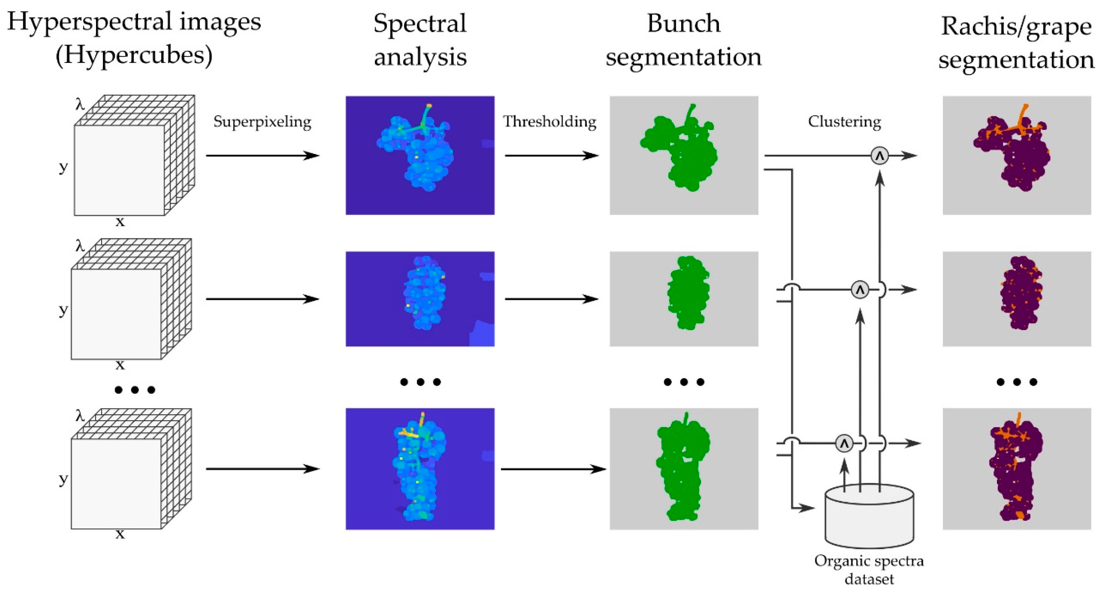
The grape area of each image was segmented following a non-supervised procedure. The whole image segmentation workflow is illustrated in
Figure 1.
Initially, the grapevine bunch was segmented using the algorithm presented in [
26]. With this procedure, the whole bunch was discriminated from the background. This algorithm computes local contrast measurements for spectral comparison based on Baddeley’s metrics, from which a superpixel image is defined. Superpixel images, introduced by Ren and Malik [
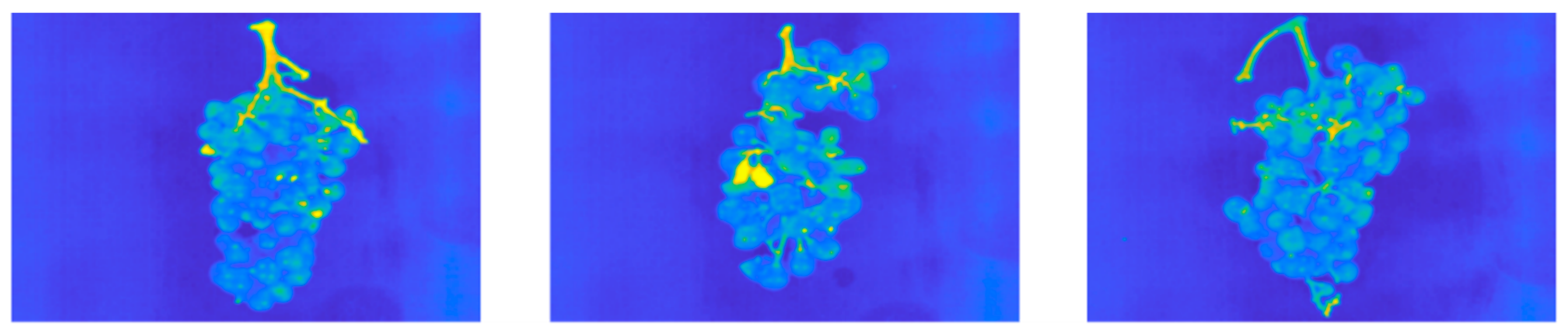
27], are oversegmented images such that each local granule is composed of pixels with similar visual features (see
Figure 1). The final binary region was produced by using the Otsu threshold determination algorithm [
28] and basic morphological operations. Pixels with (at least) 2% of the spectra in maximum values were considered as saturated, and hence removed from the selected area.
A relevant problem found in data gathering was the negative interference of the rachis when analyzing spectral information. In order to restrict the analysis to the grape areas of the bunch, a procedure was used to remove rachis areas from the segmented region. This procedure was hampered by two facts: firstly, not all images had a visible rachis; secondly, the spectral print of the rachis varied over the images due to differences in rachis lignification level and/or physical setup (e.g., angle w.r.t. the camera). Finally, we decided to perform two-class clustering (two-means, Euclidean distance) over the spectra in all images in the dataset. Only spectra in the range 1295–1311 nm were used for the procedure, since they held significant differences from rachis/grape determination. We chose a restricted range of the available spectra to be sure that the (unsupervised) clustering algorithm exclusively used information that allowed rachis and grape to be discriminated. Including all spectra might have led to unexplainable results, given the difficulties in tracking the results of multivariate two-means clustering over large datasets. The specific choice of the range 1295–1311 nm is further explained in
Figure 2. The clustering was performed globally (not individually for each image) and resulted in an almost-complete removal of rachis areas in the images in which the rachis was visible. In
Figure 1 the initial bunch segmentation can be seen to include the rachis, which were subsequently removed by the clustering procedure. This procedure resulted in the elimination of the vast majority of the rachis areas. While some grape areas were also deleted (mainly, external and shaded, semi-occluded grapes), such a collateral effect was negligible, since the final area selection included enough grape areas with no interference from the rachis.
After grape area segmentation, the relevant spectral data were extracted by unfolding the 3D hyperspectral array (hypercube) into a two-dimensional data matrix of the berry pixel reflectance values at the selected wavelengths (206 bands, from 1057 to 1700 nm). In this study, the whole dataset was randomly divided into calibration and validation groups, comprising two-thirds and one-third of images of each class, respectively. For each of the 20 bunches (10 images per class) that composed the calibration group, 15 pixels were manually selected using the graphical user-friendly interface HYPER-Tools [
29] and the RGB images of each corresponding bunch were taken as the reference. For the healthy class, 150 visually healthy pixels were selected, while 150 pixels with visible powdery mildew symptoms were selected for the infected class. The resultant matrix (300 rows × 206 columns) was used as the calibration dataset for the classification model building phase. The remaining 10 images (5 samples per class) were used as the validation dataset, hypercube unfolding was automatically performed and one matrix including the berry pixels contained in the segmented mask was obtained for each sample. Matrices were comprised of 4,350–9,600 pixels per bunch in the infected class and 15,500–19,400 pixels per bunch in the healthy one.
2.4. Multivariate Data Analysis
Data analysis was performed using the PLS_Toolbox version 8.6 (Eigenvector Research Inc., Wenatchee, WA, USA) within the MATLAB® computational environment.
2.4.1. Spectral Pre-Processing
Hyperspectral NIR data are characterized by their complexity and high dimensionality, containing not only sample information but also background information and noise. To deal with these uninformative spectra from light scattering and noise effects, mathematical pre-processing of the spectral data is preferred [
30]. Thus, useful information would be extracted to improve the subsequent data and exploratory analysis along with multivariate model development [
31].
In this study, different spectral pre-processing techniques were tested to remove instrumental noise and scattering effects, and to correct for baseline drifts and overlapping peaks in the spectra [
31,
32]. These included mean centering (MC), smoothing (SM), Multiplicative Scatter Correction (MSC), Standard Normal Variate (SNV), and first and second derivatives (1st Der and 2nd Der, respectively). Mean centering comprises of subtracting the mean spectrum of the dataset from each measured spectrum. The smoothing technique allows noise reduction and, in this case, a 15 point Savitzky–Golay [
33] filtering operation was applied to the data. MSC and SNV are the most common scatter-corrective methods used to compensate for additive and multiplicative effects in the spectra. MSC smooths out the scattering effects by linearizing each measured spectrum onto a reference spectrum, which in this particular study was the mean spectrum of the calibration dataset. SNV obtains the corrected spectrum by subtracting its mean value and dividing by its standard deviation. Derivatives can also correct for both additive and multiplicative effects. The first derivative removes baseline drift in the data, whereas the second also removes overlapping peaks. Both derivatives were computed using the Savitzky–Golay method by a second-order polynomial and 15 window points. The spectral pre-processing techniques were evaluated both individually and jointly, in order to enhance the performance of the classification model.
2.4.2. Exploratory Data Analysis
A Principal Component Analysis (PCA) was carried out to (a) explore the spectral variation within the data structure, (b) visualize any possible segregation, and (c) identify outliers in the dataset. PCA is an unsupervised projection method that aims to represent the existing variation in the dataset using a small number of uncorrelated variables, the so-called Principal Components (PC) [
34]. These PCs are a linear combination of the original variables, and remain orthogonal to each other, in such a way that first PC retains as much variance from original data as possible and so on.
In this study, PCA was used for each combination of pre-processing techniques. Their analysis was carried out by examining the PC score and loading line plots.
2.4.3. Pixel Classification
The datasets, after extraction and correction, were analyzed using Partial Least Squares Discriminant Analysis (PLS-DA), which yielded a classification model for the distinction of healthy and infected pixels within grape bunches. PLS-DA is a chemometric supervised technique for dimension reduction and discrimination in which a PLS regression is carried out to predict class membership on the calibration spectral dataset [
35]. For this, a binary dummy matrix (Y) of the two classes needs to be created, indicating class membership (1) or non-membership (0). In this study, PLS-DA models were calculated on the calibration data matrix (300 × 206 dimension) described above (
Section 2.3), using a single Venetian blinds cross-validation (CV) (10 data splits) method to choose the optimal number of Latent Variables (LV). One PLS-DA model was performed for each of the pre-processing techniques tested. Moreover, Variable Importance in Projection (VIP) scores were calculated from the most accurate PLS-DA classification model in order to select the best spectral variables for healthy and infected pixels discrimination and thus, to reduce the number of wavelengths. VIP scores estimate the importance of each variable to the model training, considered as those making the highest contribution to the PLS-DA model the ones with a VIP score close or greater than 1. The PLS-DA model was recalculated after subselecting the effective variables. The validation dataset (berry pixel matrices of the remaining 5 bunches images per class) was only used for the independent external validation of the best performing PLS-DA model. Pixel membership was predicted over each sample, generating a classification image per bunch in which predictable-infected areas were visualized.
The bunch classification was based on a pixel-wise voting majority at each image. This voting was produced from the pixel-wise classification of the pixels in the grape area at each image. Hence, the existence of contradictory information was likely to occur in the same bunch. This was mostly due to the appearance of healthy spectra in the infected bunches, as some areas might not yet be infected at the time of data gathering. The opposite (pixels classified as infected in healthy bunches) was generally due to classification errors. Nevertheless, such contradictory information was easily dealt-with in the majority voting schema, as it can be seen in our results.
The performance of the PLS-DA models was evaluated in terms of the overall classification accuracy, by the percentage of Correctly Classified (%CC) pixels and the sensitivity and specificity of each class in the CV dataset. Classification accuracy and class sensitivity and specificity parameters were calculated according to Equations (2)–(4), respectively [
36].
where TP (True Positive) is the number of healthy pixels correctly classified as healthy, TN (True Negative) is the number of infected pixels correctly classified as infected, FN (False Negative) is the number of healthy pixels incorrectly classified as infected, and FP (False Positives) is the number of infected pixels incorrectly classified as healthy. For best performance of the PLS-DA models, the accuracy should be close to 100% and the sensitivity and specificity should be close to 1.
Furthermore, the percentage of predicted pixels per class obtained on each sample in the external validation was used.
3. Results
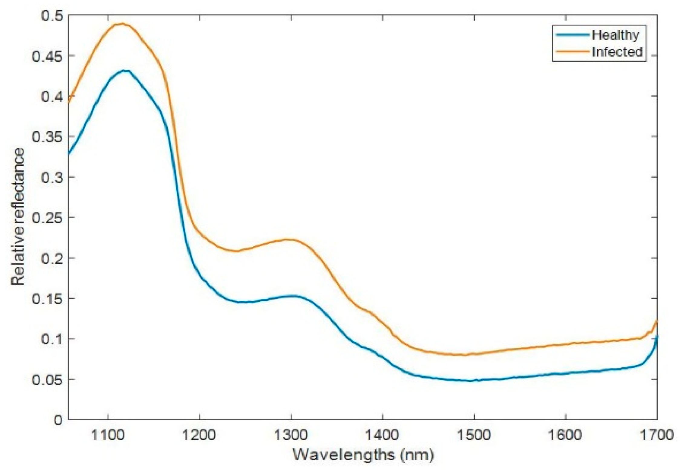
Figure 3 shows the mean reflectance spectra of the pixels selected from healthy and infected bunches in the calibration dataset. Differences in the magnitude of reflectance of both classes are noticeable along the spectral range shown. Infected pixels showed higher reflectance values than pixels selected from healthy bunches. Moreover, reflectance valleys around 1200 and 1440 nm due to absorption of water [
37] were observed in the raw reflectance spectra of the classes.
The differences in the reflectance spectra between classes could be explained from the differences in water content of the berries. It should be noted that irrespective of their powdery mildew status, healthy and infected bunches were morphologically similar, except for the bunch size which was larger in the healthy ones. In this respect, mean weight of infected bunches was significantly lower than that of healthy bunches (84.4 versus 200.8 g; F = 26.98,
p < 0.0001). However, we hypothesized that the affected berries could have dried out because of a fungal infection and, therefore, infected pixels showed higher reflectance (lower absorbance) at the absorption water bands [
38].
3.1. Principal Component Analysis (PCA)
After spectral pre-processing of the calibration dataset, a principal component analysis was carried out in order to explore the spectral variation of the two classes (healthy and infected) and to look for spectral outliers. As stated before, as many PCAs as combinations of pre-processing techniques were performed to visually separate healthy from infected pixels by means of the scores plot.
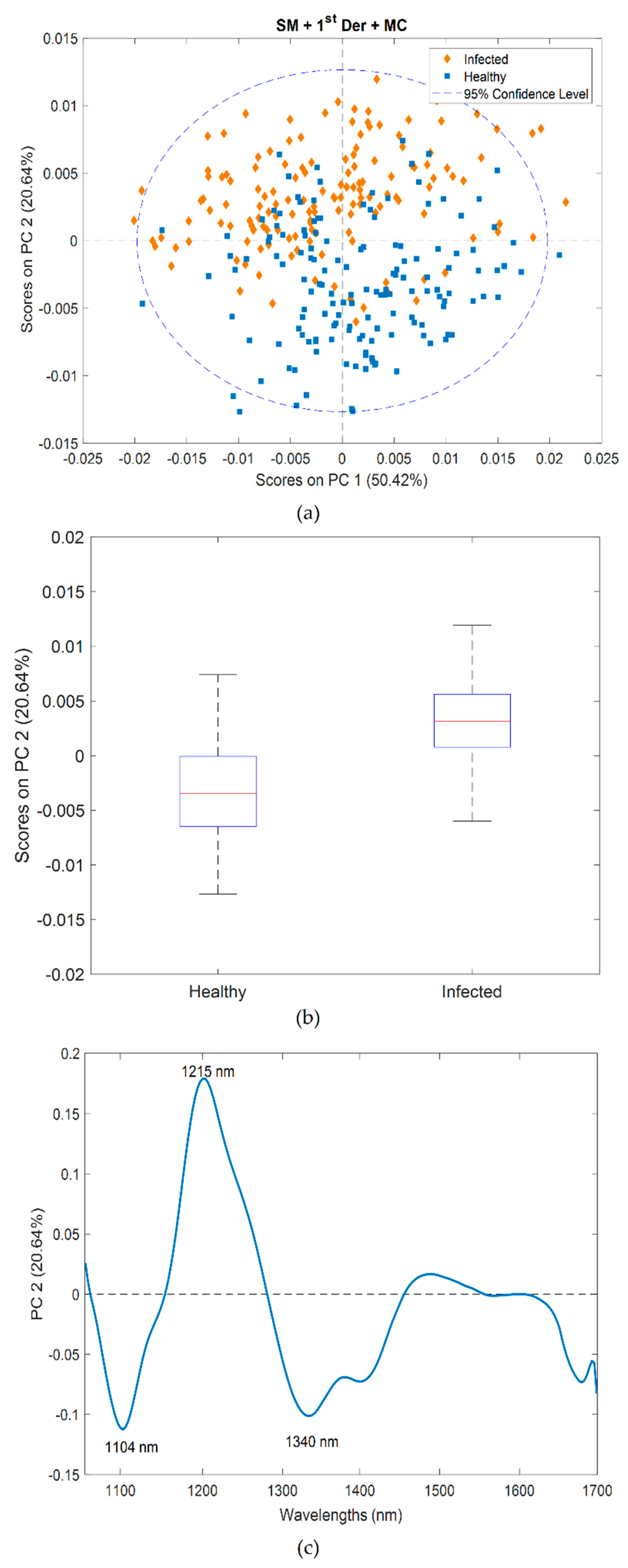
The combination of Savitzky–Golay smoothing (15-point window) followed by Savitzky–Golay 1st derivative (2nd order polynomial, 15 points) and mean centering was found to be the best data pre-processing method for class separation. Two outliers were identified and removed and the PCA was recalculated. The three principal components, accounting for 87.72% of the variance, were selected.
Figure 4a displays the score plot of PC1 (50.42%) vs. PC2 (20.64%), illustrating that the spectral variation of healthy and infected samples was best explained by the second component.
Figure 4b shows a boxplot of PC2 scores for healthy vs. infected pixels. The mean score value was negative for healthy pixels and positive for infected pixels (
Figure 4b). However, maximum score values of healthy pixels overlapped with the score values of infected pixels, and, smallest score values of the latter overlapped with healthy scores (
Figure 4b) indicating some misclassification of pixels.
The PC2 loadings plot (
Figure 4c) showed interpretable bands at 1215 nm (positive) and at 1104 nm and 1340 nm (negative). The band at 1104 nm could be associated with the C-H stretch second overtone found in aromatic groups [
37]. The bands at 1215 nm (C-H stretch second overtone) and at 1340 nm are associated with methylene groups (CH
2) and methyl groups (CH
3), respectively [
37].
3.2. PLS-DA
For this study, 10 PLS-DA models were developed using the same pre-processing combinations applied in the PCA. As explained in
Section 2.4.3, models were evaluated in terms of overall accuracy, percentage of correctly classified pixels and sensitivity/specificity for each class (healthy and infected).
A two-column binary matrix (Y) was created for analyses where samples belonging to the healthy class were described by the vector [1 0] and samples from the class infected by the [0 1] vector.
Table 1 includes, for each pre-processing combination: the number of samples used (N) after the elimination (if any) of outliers; the number of wavelengths (λ), either 206 (full spectrum) or 68 (VIP scores); the LV used; the percentage of variance explained by each model; the %CC samples of each class and the overall classification accuracy obtained in the CV dataset. Rates of classification above 80%CC were obtained for both classes regardless of the pre-processing combination used.
The best classification results were achieved for the combination of SM + SNV + MC, which resulted in an accuracy over 85% (see
Table 1). The number of LV was set to the one minimizing the mean squared error of calibration and CV [
39]. For this pre-processing combination, 5 LVs were chosen to build the classification model, accounting for 97% of explained variance.
The last row of
Table 1 displays the result of the PLS-DA model built using the effective wavelengths obtained with the VIP score method. These covered the following ranges: from 1057 to 1075 nm; 1145 to 1207 nm; 1229 to 1339 nm and 1690 to 1700 nm (68 wavelengths in total). The SM + SNV + MC pre-processing combination was the one used to build the model, as it was the best performing alternative when using the full spectrum. However, as it can be seen in
Table 1, the model using the wavelengths with a VIP score greater than 1 did not perform better in terms of accuracy than any of the other models using the full spectrum.
In
Table 2, sensitivity and specificity values of both classes after SM + SNV + MC pre-processing combination are displayed. Sensitivity was slightly higher for the infected class than for the healthy one, meaning that infected pixels were better classified into their corresponding class (TN) than healthy pixels.
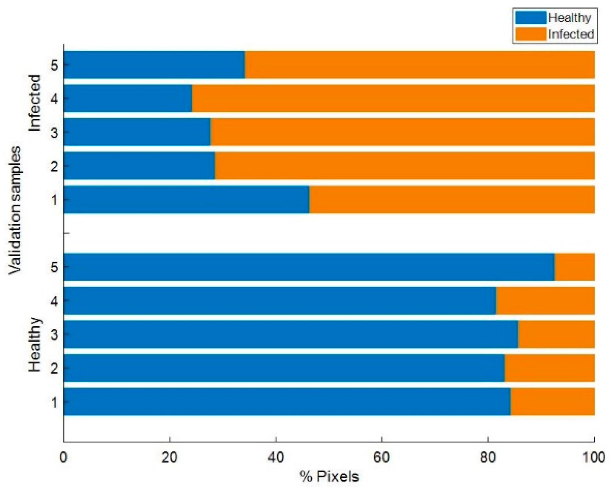
Figure 5 shows the results obtained for the model external validation performed for each sample of the validation dataset (10 bunches) independently. Only the PLS-DA model built using SM + SNV + MC combination was used for the external validation of samples.
Figure 5 displays the percentage of pixels classified as either healthy or infected in each validation sample obtained from the probability of each of the pixels belonging to the classes considered.
In all 10 samples, a high proportion of pixels were correctly classified into their corresponding class. In general, a higher correct classification rate was achieved for healthy pixels than for powdery mildew affected pixels unlike the previous case for the CV dataset. In any case, an average 85.70% of pixels from the five bunches belonging to the healthy class were correctly identified as healthy (TP); and, 68.34% pixels from the five infected bunches were correctly labeled as infected (TN). These results are meaningful inasmuch as an infected bunch might have areas where the level of infection is null or insignificant. In other words, a diseased bunch may not necessarily have all berries covered by the Erysiphe necator fungus mycelia.
It should be noted that the difficulty in the pixel-wise external validation, mainly due to the impossibility of labeling individual pixels, resulted in some false negatives and false positives, that is to say, some healthy pixels were classified as infected and vice versa. In any case, bunches could be easily sorted into groups by establishing a tolerance threshold; in this particular case a loose threshold of 20% could be established denoting that bunches with more than 20% of pixels identified as infected could be considered sick and bunches with less than 20% of pixels classified as infected be considered healthy. Whereas a better pixel-wise classification might be desired or needed for other applications, e.g., data-driven models of fungal growth over time,
Figure 5 illustrates how it is clearly functional for the present goal of whole-bunch classification for powdery mildew detection.
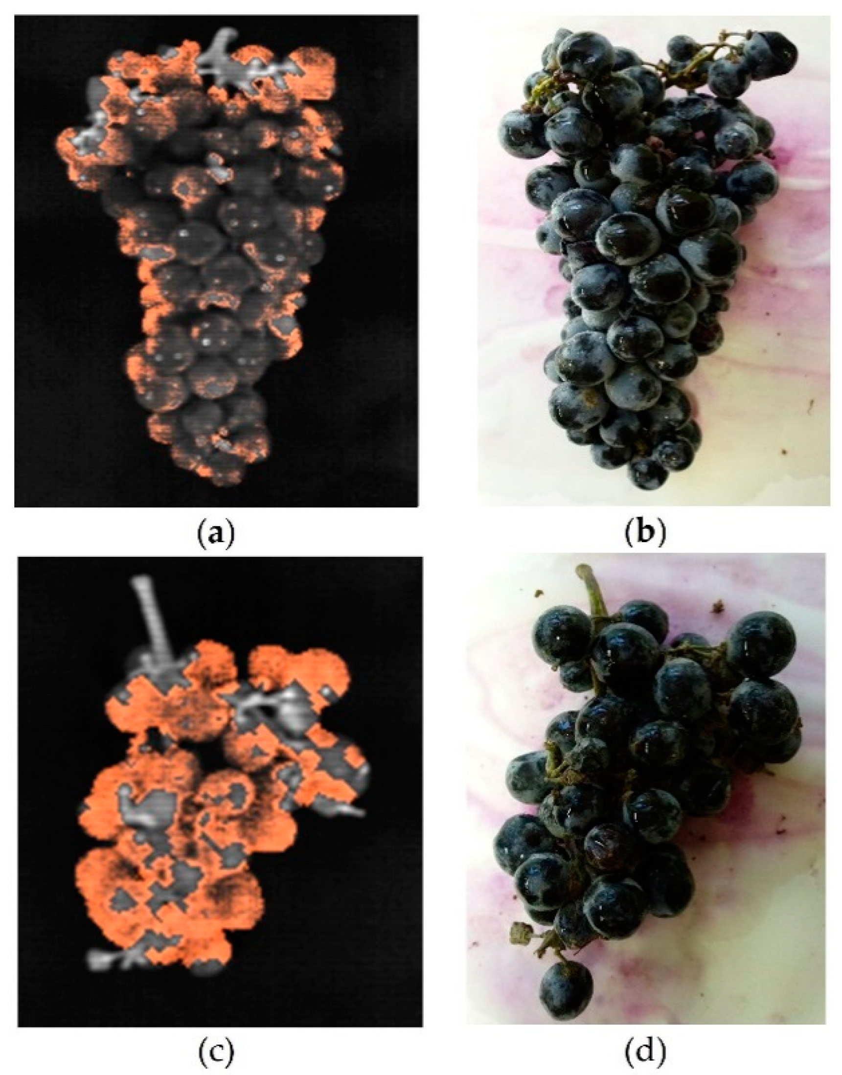
Figure 6 shows a display of the classification of pixels in two bunches (validation sample 1 and 4 of healthy and infected classes, respectively). Images on the left were obtained by the HSI system showing in orange the pixels classified as infected (
Figure 6a,c). In the same way, images on the right correspond to the RGB images of the same bunches taken as the reference (
Figure 6b,d). For instance,
Figure 6a shows a healthy bunch for which 15.71% of pixels were labeled as infected and
Figure 6c displays an infected bunch with 75.77% of pixels correctly classified to the class they belonged to. It is important to note the spatial coherence of the classification of pixels in the images. Thus, as seen in
Figure 6a, false negative pixels were mostly located on the sloping surfaces of the berries. At the same time, berries illuminated correctly, with a visible surface perpendicular to the HSI system barely presented false negative pixels. This fact suggests that the existence of powdery mildew in the bunch produces a noticeable effect on the spectrum acquired in the berries, which, although can be mistaken with other physical events (lighting, inclination, etc.), makes it clearly distinguishable from non-sick berries.
4. Discussion
The detection of grapevine diseases, both in field and laboratory conditions, using different spectroscopic techniques has been somewhat explored in the last decade. Naidu et al. [
40] studied the potential of spectral reflectance to diagnose grapevine leafroll disease (GLD). Authors recorded in situ leaf reflectance spectra of 241 detached leaves of two wine grape cultivars (Cabernet Sauvignon and Merlot) including healthy and infected samples showing GLD symptoms and known to be infected with grapevine leafroll-associated virus-3 (GLRaV-3). A portable spectrometer (350–2500 nm) was used to acquire leaf spectral reflectance and a reverse transcription-polymerase chain reaction (RT-PCR) was carried out for virus detection. Discriminant analyses based on single and multiple variables were performed. The best classification results of healthy and infected leaves were obtained using multiple variables, with an overall accuracy of 0.81.
A similar study conducted by the same team was recently published [
41]. In this work, the objective was also to classify healthy and GLD-diseased grapevines leaves, and the spectral measurements of cv. Cabernet Sauvignon leaves were taken non-destructively in the field in two consecutive seasons (2016 and 2017). Spectral measurements of 60 healthy and 60 GLD-infected (30 symptomatic and 30 asymptomatic) leaves were acquired at three different moments in 2016 (pre-veraison, 2-weeks post-veraison and 4-weeks post-veraison), whereas approximately 60 healthy and 120 GLD-infected (60 symptomatic and 60 asymptomatic) leaves were measured at the same three moments in 2017. A portable VIS-NIR spectroradiometer (350–2500 nm) was used for a spectral recording and a RT-PCR to ascertain GLRaV-3 presence. A quadratic discriminant analysis yielded overall classification accuracies between 75–99% in both seasons. Therefore, authors concluded that spectral reflectance in the VIS-NIR range was suitable for non-destructive detection of GLRaV-3 under field conditions in cv. Cabernet Sauvignon grapevines.
Petrovic et al. [
42] investigated the discrimination of powdery mildew-affected grape berries at harvest by attenuated total reflection (ATR) mid-infrared (MIR) spectroscopy and fatty acid analysis. Spectra of 138 individual berries detached from 30 bunches (25 designated powdery mildew-affected and 5 visually healthy) were collected in the range 4000–400 cm
−1. From the 138 berries, 61 were selected for fatty acid analysis. A forward selection stepwise linear discriminant analysis (SLDA) was performed to separate healthy from infected berries. Authors found that the analysis of fatty acids gave better results of classification than MIR. The discriminant analysis of four saturated fatty acids achieved a classification accuracy of 97% for healthy berries and 75% of powdery mildew-affected samples whereas 82% of berries were correctly classified using ATR-MIR.
Likewise, the potential of HSI to detect different diseases in grapevine has been investigated over the last few years. Oerke et al. [
10] studied the changes in the hyperspectral signature of downy mildew affected leaves compared to healthy leaves. Cultivars Mueller-Thurgau (highly susceptible), Regent and Solaris (both resistant) were used in the study. For each cultivar, between 15 and 20 plants were inoculated with
Plasmopara viticola and incubated for 24 h at 100% RH. Hyperspectral images were acquired in the 400–1000 nm spectral range. The Spectral Angle Mapper (SAM) algorithm was used to distinguish image pixels of healthy and infected leaves. Authors reported a considerable variation in the reflectance spectra of leaf tissue of non-inoculated and
Plasmopara viticola-inoculated leaves of Mueller-Thurgau cultivar.
MacDonald et al. [
21] evaluated the accuracy of remote hyperspectral imaging detection of GLRaV-3 in Cabernet Sauvignon vineyards. Images were acquired with a hyperspectral camera sensitive in the 400–1000 nm spectral range in five vineyards over two years. At the same time, visual assessment of disease was conducted in the same field, and the virus was tested with the RT-PCR method, confirming the accuracy of the visual estimation (98%). Visual mapping was then compared to the hyperspectral image for each vineyard using the Classification and Regression Tree (CART) algorithm. An overall accuracy of 94.1% was achieved in the detection of GLRaV-3.
In this study, we focused on the combination of hyperspectral imaging and chemometric analysis to identify the powdery mildew infection in cv. Carignan Noir (syn. Mazuelo) grape bunches on a laboratory scale. Other authors have explored to some extent the assessment of the presence of powdery mildew using HSI systems. Oberti et al. [
5] studied the automatic detection of powdery mildew fungal disease by multispectral imaging analysis of grapevine leaves. Plants of Cabernet Sauvignon cultivar grown under controlled conditions in a greenhouse were inoculated with
Erysiphe necator, and images of their leaves were acquired 4, 8 and 16 days after inoculation. Images were taken with an R-G-NIR multispectral camera, and recorded in three spectral channels: red (540 nm), green (660 nm) and near-infrared (800 nm). In total, 35 different leaf samples with different stages of infection were measured at five different angles per leaf (from 0° to 75°). Authors concluded that sensitivity values generally improved as the view angle was increased. In addition, sensitivity values between 61–97% were achieved for all angles at advanced stages of infection. Despite the good classification results achieved and due to the nature of the technology used, the authors could not provide an image of the leaves displaying the affected areas.
A different approach was adopted by Beghi et al. [
24] who evaluated the phytosanitary status of grape bunches while entering the winery using visible and NIR conventional spectroscopy. Healthy and diseased bunches (2559 in total) were measured in the 400–1650 nm spectral range using a non-contact device. It should be noted that diseased bunches comprised different pathologies like botrytis, powdery mildew and sour rot and, therefore, specific results for powdery mildew were not obtained. In any case, very good classification rates were achieved in the test set with an accuracy above 89% in the PLS-DA model developed.
In a study more similar to the one presented here, Knauer et al. [
23] improved the classification accuracy of powdery mildew in grapevine bunches using a spatial–spectral segmentation approach. The dataset comprised 30 bunches of Chardonnay vines collected shortly before veraison. Bunches were visually divided into three categories: healthy, powdery mildew infected, and severally diseased, comprising 10 bunches per class. Then, a modified duplex quantitative polymerase chain reaction (qPCR) was used to detect and quantify
Erysiphe necator fungus. Hyperspectral images of samples were acquired using two cameras, a visible and near-infrared (VNIR) camera from 400 to 1000 nm; and, a short-wave infrared (SWIR) camera covering the 970–2500 nm range. A dimensionality reduction by Linear Discriminant Analysis was accomplished and a subsequent classification based on modified Random Forest was carried out. Authors reported no possible successful classification in the SWIR range. For VNIR hyperspectral images, they achieved an accuracy of 87% in the classification of the three categories of samples. These results were in accordance with the ones obtained here in the CV dataset (87% vs. 85.33%). Moreover, they obtained more than 80% of true positive pixels (healthy pixels classified as healthy) as it was in our case with 85.70% of TP pixels in the validation dataset. However, the complexity in the image processing of our study should be valued compared to the latter due to the use of black berries. Segmentation of black grape bunches is an intricate task that we were able to accomplish successfully. To our knowledge, this represents the first study that assesses the use of HSI to classify powdery mildew affected bunches of a black-berried cultivar, and thus it may open a new niche of study.
We consider that the results presented here pave the way to future investigation within this research line, although the study has certain limitations. Even though the threshold we suggested is probably not sensitive enough for individual bunch classification, it may constitute a very useful starting point when classifying a grape batch or qualifying a vineyard. The possibility of using data fusion techniques could be considered to improved classification results. Some authors have explored the opportunity to use image fusion methods to tackle complex tasks such as: on-site fruit detection [
43], identification of plant stress [
44], detection of plant diseases [
45], and forest monitoring [
46] among others.
Future investigation of this topic should include a larger dataset and preferably composed of fresh (not frozen) samples to mimic end-user suitable conditions. Moreover, quantification of Erysiphe necator biomass by means of a qPCR is highly advisable to confirm that only powdery mildew is being assessed and no other diseases or abiotic stresses are being analyzed. Besides, upcoming studies should focus on the identification of a few optimal wavelengths to identify powdery mildew infection that could reduce the processing time while avoiding confounding information from other quality parameters. Thus, allowing the development of image-based sensors for the real time detection of powdery mildew infection in the field.

 ,
, 


