
Prediction of Neutralization Depth of R.C. Bridges Using Machine Learning Methods


Abstract
1. Introduction
2. Dataset Description and Analysis
3. Parameter Evaluation and Selection
3.1. Random Forest for Parameter Evaluation
3.2. Results and Discussions
4. Machine Learning Models
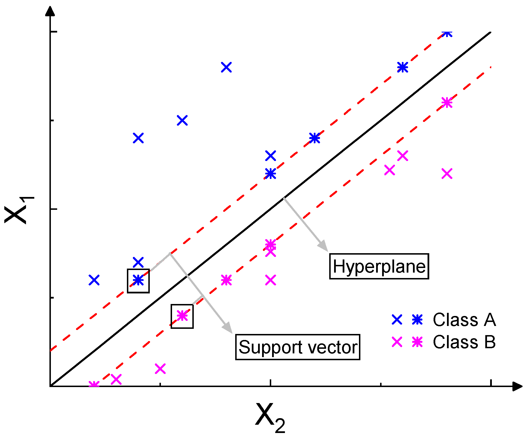
4.1. Support Vector Machine
4.2. K-Nearest Neighbor
4.3. AdaBoost
4.4. XGBoost
4.5. Multi-Class Problem
4.6. Results and Discussions
5. Conclusions
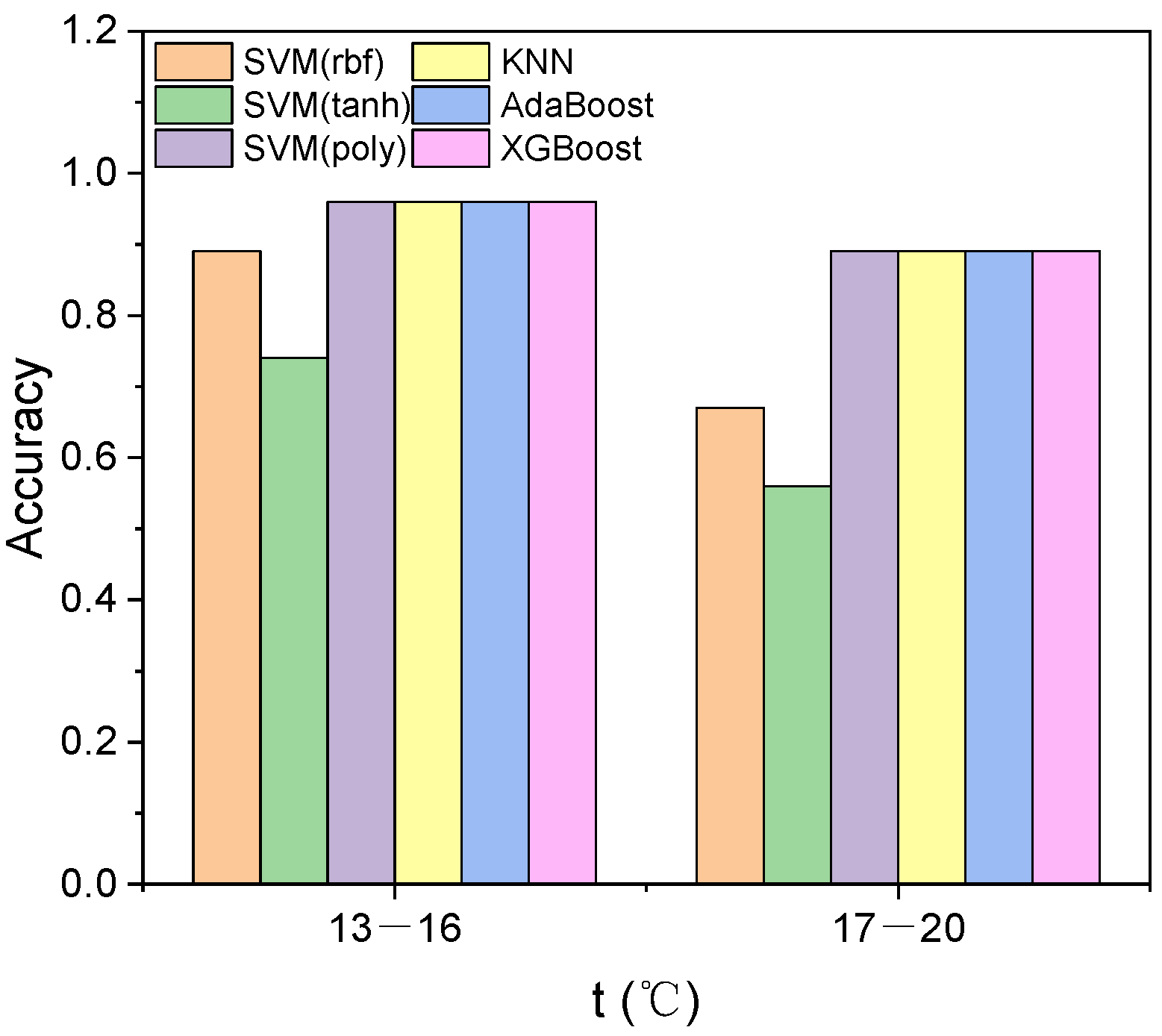
- This study used SVM, KNN, AdaBoost and XGBoost to predict the neutralization depth level of the concrete of existing bridges, and the results show that the radial basis kernel SVM model has the highest validation accuracy (91%) and the highest macro recall rate (86%), with only four parameters. The radial basis kernel function is the best kernel functions in this study. Compared with other models, the radial basis kernel SVM model and KNN model achieve a better performance;
- The results reveal the preference of ML methods. KNN is good at classifying slight-level samples (accuracy > 97%), and AdaBoost is the best method for the prediction of medium-level samples (accuracy > 93%). Machine learning shows great potential in predicting the neutralization depth of concrete with very few parameters, and evaluating the durability level of existing bridges;
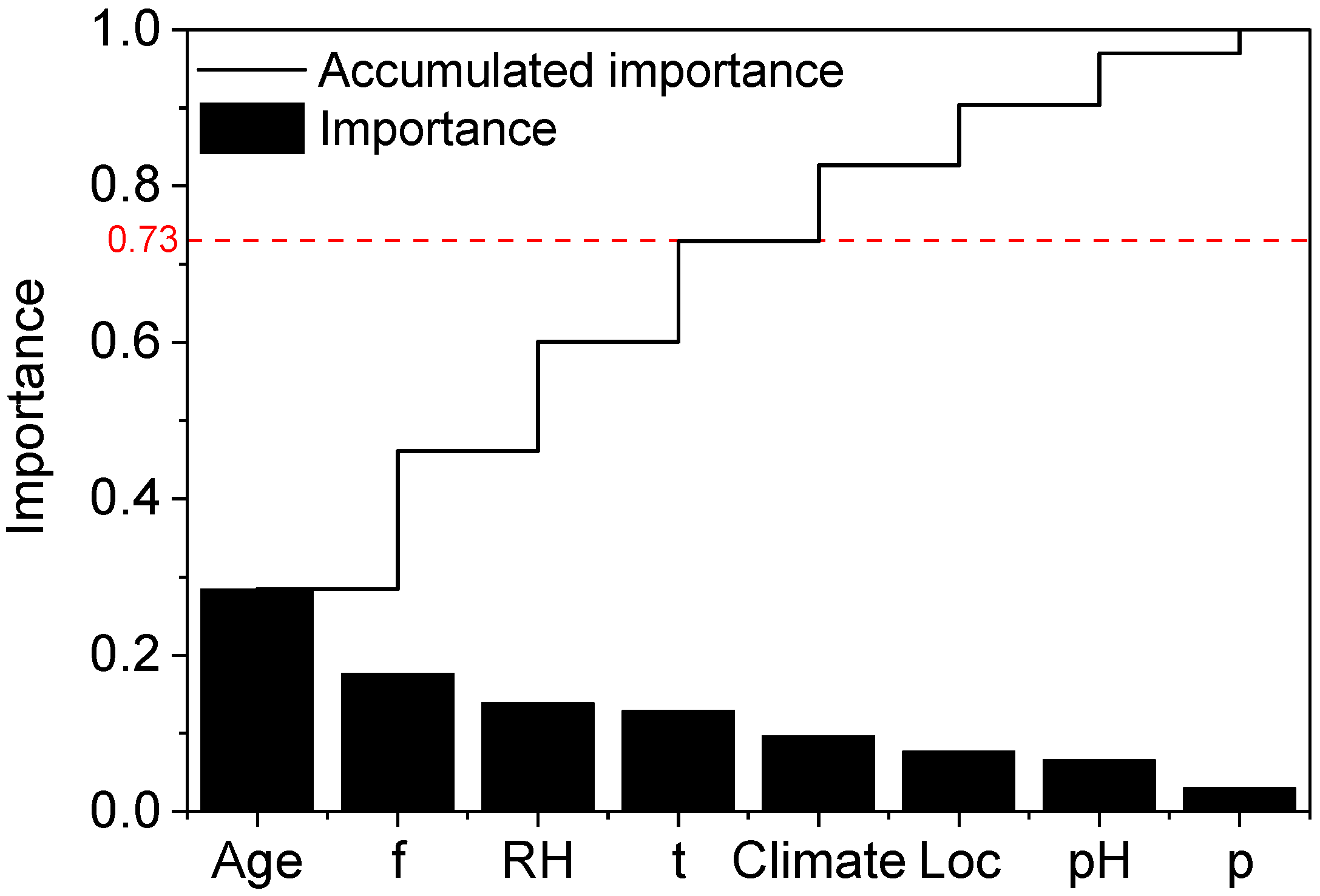
- Random forest was used for parameter selection. The results show that temperature, concrete strength, RH and service time are more important than climate, acid rain, location of components, and load level. The cumulative importance of these top four parameters reaches 73%. The performance of the models shows that random forest is an effective approach for parameter selection.
Author Contributions
Funding
Institutional Review Board Statement
Informed Consent Statement
Data Availability Statement
Conflicts of Interest
Appendix A

| Age | f | t | RH | pH | p | Climate | Loc 1 | d | Reference | Age | f | t | RH | pH | p | Climate | Loc 1 | d | Reference |
|---|---|---|---|---|---|---|---|---|---|---|---|---|---|---|---|---|---|---|---|
| 49 | 25 | 16 | 75 | 5 | 2 | north subtropics | Ar | 19.72 | self-test | 7 | 45 | 21.8 | 83 | 6 | 1 | edge tropics | Bpier | 2.8 | [56] |
| 49 | 35 | 16 | 75 | 5 | 2 | north subtropics | Ar | 11.48 | 7 | 45 | 21.8 | 83 | 6 | 1 | edge tropics | Bpier | 1.5 | ||
| 49 | 25 | 16 | 75 | 5 | 2 | north subtropics | Ar | 17.02 | 23 | 35 | 20.5 | 77 | 4 | 2 | south subtropics | Ar | 7.483 | [57] | |
| 49 | 20 | 16 | 75 | 5 | 2 | north subtropics | Ar | 20.23 | 23 | 45 | 20.5 | 77 | 4 | 2 | south subtropics | Ar | 5.937 | ||
| 49 | 15 | 16 | 75 | 5 | 2 | north subtropics | Ar | 16.47 | 23 | 40 | 20.5 | 77 | 4 | 2 | south subtropics | Ar | 11.453 | ||
| 49 | 20 | 16 | 75 | 5 | 2 | north subtropics | Ar | 20.23 | 23 | 45 | 20.5 | 77 | 4 | 2 | south subtropics | Ar | 4.917 | ||
| 49 | 25 | 16 | 75 | 5 | 2 | north subtropics | Ar | 11.11 | 23 | 50 | 20.5 | 77 | 4 | 2 | south subtropics | Ar | 4.35 | ||
| 49 | 20 | 16 | 75 | 5 | 2 | north subtropics | Ar | 12.15 | 23 | 35 | 20.5 | 77 | 4 | 2 | south subtropics | Ar | 4.563 | ||
| 49 | 25 | 16 | 75 | 5 | 2 | north subtropics | Ar | 16.38 | 23 | 60 | 20.5 | 77 | 4 | 2 | south subtropics | Ar | 4 | ||
| 49 | 15 | 16 | 75 | 5 | 2 | north subtropics | Ar | 23.45 | 23 | 60 | 20.5 | 77 | 4 | 2 | south subtropics | Ar | 3.577 | ||
| 49 | 20 | 16 | 75 | 5 | 2 | north subtropics | Ar | 20.62 | 23 | 55 | 20.5 | 77 | 4 | 2 | south subtropics | Ar | 3.673 | ||
| 49 | 15 | 16 | 75 | 5 | 2 | north subtropics | Ar | 21.57 | 23 | 55 | 20.5 | 77 | 4 | 2 | south subtropics | Ar | 4.12 | ||
| 49 | 30 | 16 | 75 | 5 | 2 | north subtropics | Bpla | 8.4 | 23 | 50 | 20.5 | 77 | 4 | 2 | south subtropics | Ar | 3.63 | ||
| 49 | 30 | 16 | 75 | 5 | 2 | north subtropics | Bpla | 8.4 | 23 | 55 | 20.5 | 77 | 4 | 2 | south subtropics | Ar | 3.56 | ||
| 49 | 30 | 16 | 75 | 5 | 2 | north subtropics | Bpla | 5.43 | 23 | 50 | 20.5 | 77 | 4 | 2 | south subtropics | Ar | 4.343 | ||
| 49 | 30 | 16 | 75 | 5 | 2 | north subtropics | Bpla | 5.43 | 23 | 50 | 20.5 | 77 | 4 | 2 | south subtropics | Ar | 3.853 | ||
| 49 | 15 | 16 | 75 | 5 | 2 | north subtropics | Bpier | 18.55 | 23 | 60 | 20.5 | 77 | 4 | 2 | south subtropics | Ar | 4.497 | ||
| 49 | 15 | 16 | 75 | 5 | 2 | north subtropics | Bpier | 18.55 | 23 | 50 | 20.5 | 77 | 4 | 2 | south subtropics | Ar | 5.067 | ||
| 19 | 55 | 16 | 75 | 5 | 1 | north subtropics | Bm | 1 | 23 | 60 | 20.5 | 77 | 4 | 2 | south subtropics | Ar | 3.3 | ||
| 19 | 45 | 16 | 75 | 5 | 1 | north subtropics | Bm | 1.5 | 23 | 55 | 20.5 | 77 | 4 | 2 | south subtropics | Ar | 3.267 | ||
| 19 | 50 | 16 | 75 | 5 | 1 | north subtropics | Bm | 2 | 23 | 55 | 20.5 | 77 | 4 | 2 | south subtropics | Ar | 4.453 | ||
| 19 | 55 | 16 | 75 | 5 | 1 | north subtropics | Bm | 1.5 | 23 | 45 | 20.5 | 77 | 4 | 2 | south subtropics | Ar | 4.097 | ||
| 19 | 50 | 16 | 75 | 5 | 1 | north subtropics | Bm | 2 | 23 | 55 | 20.5 | 77 | 4 | 2 | south subtropics | Ar | 4.47 | ||
| 19 | 50 | 16 | 75 | 5 | 1 | north subtropics | Bm | 1.5 | 23 | 50 | 20.5 | 77 | 4 | 2 | south subtropics | Ar | 4.31 | ||
| 19 | 35 | 16 | 75 | 5 | 1 | north subtropics | Bm | 1 | 23 | 45 | 20.5 | 77 | 4 | 2 | south subtropics | Ar | 5.18 | ||
| 19 | 50 | 16 | 75 | 5 | 1 | north subtropics | Bm | 1 | 23 | 45 | 20.5 | 77 | 4 | 2 | south subtropics | Ar | 4.7 | ||
| 19 | 45 | 16 | 75 | 5 | 1 | north subtropics | Bm | 1 | 23 | 20 | 20.5 | 77 | 4 | 2 | south subtropics | Ar | 14.773 | ||
| 19 | 45 | 16 | 75 | 5 | 1 | north subtropics | Bm | 1 | 23 | 45 | 20.5 | 77 | 4 | 2 | south subtropics | Ar | 3.85 | ||
| 19 | 40 | 16 | 75 | 5 | 1 | north subtropics | Bm | 1 | 23 | 40 | 20.5 | 77 | 4 | 2 | south subtropics | Ar | 4.513 | ||
| 19 | 45 | 16 | 75 | 5 | 1 | north subtropics | Bm | 0.5 | 23 | 45 | 20.5 | 77 | 4 | 2 | south subtropics | Ar | 4.467 | ||
| 19 | 40 | 16 | 75 | 5 | 1 | north subtropics | Bm | 0.5 | 23 | 50 | 20.5 | 77 | 4 | 2 | south subtropics | Ar | 9.923 | ||
| 19 | 45 | 16 | 75 | 5 | 1 | north subtropics | Bpier | 1 | 23 | 50 | 20.5 | 77 | 4 | 2 | south subtropics | Ar | 6.83 | ||
| 19 | 45 | 16 | 75 | 5 | 1 | north subtropics | Bpier | 1.5 | 23 | 30 | 20.5 | 77 | 4 | 2 | south subtropics | Bpier | 16.51 | ||
| 19 | 45 | 16 | 75 | 5 | 1 | north subtropics | Bpier | 1.5 | 23 | 30 | 20.5 | 77 | 4 | 2 | south subtropics | Bpier | 6.037 | ||
| 19 | 50 | 16 | 75 | 5 | 1 | north subtropics | Bpier | 1 | 23 | 25 | 20.5 | 77 | 4 | 2 | south subtropics | Bpier | 5.857 | ||
| 19 | 40 | 16 | 75 | 5 | 1 | north subtropics | Bpier | 2 | 23 | 20 | 20.5 | 77 | 4 | 2 | south subtropics | Bpier | 6.753 | ||
| 19 | 50 | 16 | 75 | 5 | 1 | north subtropics | Bpier | 1 | 23 | 25 | 20.5 | 77 | 4 | 2 | south subtropics | Bpier | 16.21 | ||
| 19 | 45 | 16 | 75 | 5 | 1 | north subtropics | Bpier | 0.5 | 23 | 35 | 20.5 | 77 | 4 | 2 | south subtropics | Bpier | 11.597 | ||
| 20 | 40 | 16.2 | 82 | 4 | 1 | mid-subtropics | Ar | 4 | [38] | 3 | 25 | 5.8 | 65 | 6 | 2 | mid temperate zone | Bm | 6.2 | [58] |
| 20 | 45 | 16.2 | 82 | 4 | 1 | mid-subtropics | Bm | 3.5 | 3 | 25 | 5.8 | 65 | 6 | 2 | mid temperate zone | Bm | 6 | ||
| 20 | 45 | 16.2 | 82 | 4 | 1 | mid-subtropics | Bm | 3.5 | 3 | 25 | 5.8 | 65 | 6 | 2 | mid temperate zone | Bm | 6 | ||
| 20 | 40 | 16.2 | 82 | 4 | 1 | mid-subtropics | Bm | 3.5 | 3 | 25 | 5.8 | 65 | 6 | 2 | mid temperate zone | Bm | 6.5 | ||
| 20 | 40 | 16.2 | 82 | 4 | 1 | mid-subtropics | Bm | 4 | 3 | 25 | 5.8 | 65 | 6 | 2 | mid temperate zone | Bm | 5.5 | ||
| 20 | 40 | 16.2 | 82 | 4 | 1 | mid-subtropics | Bpier | 3.5 | 3 | 25 | 5.8 | 65 | 6 | 2 | mid temperate zone | Bm | 5.5 | ||
| 35 | 40 | 17.4 | 80 | 4 | 1 | mid-subtropics | Ar | 3 | [39] | 3 | 25 | 5.8 | 65 | 6 | 2 | mid temperate zone | Bm | 5.8 | |
| 35 | 25 | 17.4 | 80 | 4 | 1 | mid-subtropics | Ar | 2.5 | 3 | 25 | 5.8 | 65 | 6 | 2 | mid temperate zone | Bm | 6.2 | ||
| 35 | 40 | 17.4 | 80 | 4 | 1 | mid-subtropics | Bpla | 3 | 20 | 25 | 14.4 | 72 | 6 | 1 | warm temperate | Bm | 9.7 | [59] | |
| 35 | 45 | 17.4 | 80 | 4 | 1 | mid-subtropics | Bm | 1.5 | 20 | 35 | 14.4 | 72 | 6 | 1 | warm temperate | Bpier | 11.2 | ||
| 32 | 45 | 16.2 | 78 | 4 | 2 | north subtropics | Ar | 8.53 | [40] | 12 | 30 | 22.7 | 76 | 5 | 2 | south subtropics | Bm | 1.68 | [60] |
| 32 | 45 | 16.2 | 78 | 4 | 2 | north subtropics | Ar | 8.63 | 12 | 35 | 22.7 | 76 | 5 | 2 | south subtropics | Bm | 1.46 | ||
| 32 | 45 | 16.2 | 78 | 4 | 2 | north subtropics | Ar | 8.4 | 12 | 30 | 22.7 | 76 | 5 | 2 | south subtropics | Bm | 1.63 | ||
| 32 | 40 | 16.2 | 78 | 4 | 2 | north subtropics | Ar | 8.73 | 12 | 30 | 22.7 | 76 | 5 | 2 | south subtropics | Bm | 1.53 | ||
| 32 | 40 | 16.2 | 78 | 4 | 2 | north subtropics | Ar | 8.93 | 26 | 25 | 4.2 | 62 | 6 | 1 | mid temperate zone | Bm | 7.6 | https://wenku.baidu.com/view/f66434afce2f0066f53322d8.html?sxts=1575776593501 (accessed on 20 February 2021) | |
| 32 | 40 | 16.2 | 78 | 4 | 2 | north subtropics | Ar | 9.07 | 26 | 25 | 4.2 | 62 | 6 | 1 | mid temperate zone | Bm | 9.1 | ||
| 32 | 35 | 16.2 | 78 | 4 | 2 | north subtropics | Ar | 8.7 | 26 | 30 | 4.2 | 62 | 6 | 1 | mid temperate zone | Bm | 9 | ||
| 32 | 35 | 16.2 | 78 | 4 | 2 | north subtropics | Ar | 9 | 26 | 25 | 4.2 | 62 | 6 | 1 | mid temperate zone | Bm | 9.5 | ||
| 32 | 35 | 16.2 | 78 | 4 | 2 | north subtropics | Ar | 8.6 | 26 | 25 | 4.2 | 62 | 6 | 1 | mid temperate zone | Bm | 10.2 | ||
| 32 | 35 | 16.2 | 78 | 4 | 2 | north subtropics | Ar | 8.83 | 26 | 20 | 4.2 | 62 | 6 | 1 | mid temperate zone | Bpla | 13.5 | ||
| 32 | 35 | 16.2 | 78 | 4 | 2 | north subtropics | Ar | 9.2 | 26 | 25 | 4.2 | 62 | 6 | 1 | mid temperate zone | Bpier | 9.72 | ||
| 32 | 40 | 16.2 | 78 | 4 | 2 | north subtropics | Ar | 9.2 | 26 | 20 | 4.2 | 62 | 6 | 1 | mid temperate zone | Bpier | 8.8 | ||
| 32 | 40 | 16.2 | 78 | 4 | 2 | north subtropics | Ar | 8.63 | 12 | 50 | 17.2 | 77 | 4 | 1 | north subtropics | Bm | 1.9 | https://wenku.baiducom/view/73a61a52f5335a8102d220b8.html?sxts=1575779109843 (accessed on 20 February 2021) | |
| 32 | 40 | 16.2 | 78 | 4 | 2 | north subtropics | Ar | 8.83 | 12 | 50 | 17.2 | 77 | 4 | 1 | north subtropics | Bm | 2.5 | ||
| 32 | 35 | 16.2 | 78 | 4 | 2 | north subtropics | Ar | 9.37 | 12 | 50 | 17.2 | 77 | 4 | 1 | north subtropics | Bm | 3 | ||
| 32 | 45 | 16.2 | 78 | 4 | 2 | north subtropics | Ar | 8.47 | 12 | 55 | 17.2 | 77 | 4 | 1 | north subtropics | Bm | 2.7 | ||
| 32 | 40 | 16.2 | 78 | 4 | 2 | north subtropics | Ar | 8.9 | 12 | 50 | 17.2 | 77 | 4 | 1 | north subtropics | Bm | 1.5 | ||
| 32 | 40 | 16.2 | 78 | 4 | 2 | north subtropics | Ar | 7.97 | 12 | 50 | 17.2 | 77 | 4 | 1 | north subtropics | Bm | 3.1 | ||
| 32 | 45 | 16.2 | 78 | 4 | 2 | north subtropics | Ar | 8.83 | 12 | 50 | 17.2 | 77 | 4 | 1 | north subtropics | Bm | 3.5 | ||
| 32 | 40 | 16.2 | 78 | 4 | 2 | north subtropics | Ar | 8.2 | 12 | 50 | 17.2 | 77 | 4 | 1 | north subtropics | Bm | 3 | ||
| 32 | 40 | 16.2 | 78 | 4 | 2 | north subtropics | Ar | 7.93 | 12 | 55 | 17.2 | 77 | 4 | 1 | north subtropics | Bm | 2.5 | ||
| 32 | 40 | 16.2 | 78 | 4 | 2 | north subtropics | Ar | 9.23 | 12 | 55 | 17.2 | 77 | 4 | 1 | north subtropics | Bm | 3.5 | ||
| 32 | 40 | 16.2 | 78 | 4 | 2 | north subtropics | Ar | 8.83 | 12 | 50 | 17.2 | 77 | 4 | 1 | north subtropics | Bm | 2.9 | ||
| 32 | 40 | 16.2 | 78 | 4 | 2 | north subtropics | Ar | 8.6 | 12 | 50 | 17.2 | 77 | 4 | 1 | north subtropics | Bm | 2.5 | ||
| 41 | 40 | 14.5 | 70 | 5 | 2 | warm temperate | Bm | 6 | [41] | 12 | 50 | 17.2 | 77 | 4 | 1 | north subtropics | Bm | 2.5 | |
| 41 | 40 | 14.5 | 70 | 5 | 2 | warm temperate | Bm | 9 | 12 | 55 | 17.2 | 77 | 4 | 1 | north subtropics | Bm | 1.6 | ||
| 41 | 40 | 14.5 | 70 | 5 | 2 | warm temperate | Bm | 7 | 12 | 50 | 17.2 | 77 | 4 | 1 | north subtropics | Bm | 3.8 | ||
| 41 | 40 | 14.5 | 70 | 5 | 2 | warm temperate | Bm | 8 | 12 | 50 | 17.2 | 77 | 4 | 1 | north subtropics | Bm | 3.5 | ||
| 41 | 35 | 14.5 | 70 | 5 | 2 | warm temperate | Bm | 6 | 12 | 35 | 17.2 | 77 | 4 | 1 | north subtropics | Bm | 4 | ||
| 41 | 35 | 14.5 | 70 | 5 | 2 | warm temperate | Bm | 5 | 12 | 30 | 17.2 | 77 | 4 | 1 | north subtropics | Bpier | 3.5 | ||
| 41 | 35 | 14.5 | 70 | 5 | 2 | warm temperate | Bm | 9 | 12 | 35 | 17.2 | 77 | 4 | 1 | north subtropics | Bpier | 2.5 | ||
| 41 | 30 | 14.5 | 70 | 5 | 2 | warm temperate | Bm | 5 | 12 | 30 | 17.2 | 77 | 4 | 1 | north subtropics | Bm | 2.6 | ||
| 41 | 30 | 14.5 | 70 | 5 | 2 | warm temperate | Bm | 5 | 12 | 30 | 17.2 | 77 | 4 | 1 | north subtropics | Bpier | 3.5 | ||
| 41 | 45 | 14.5 | 70 | 5 | 2 | warm temperate | Bm | 7 | 12 | 35 | 17.2 | 77 | 4 | 1 | north subtropics | Bpier | 4 | ||
| 41 | 35 | 14.5 | 70 | 5 | 2 | warm temperate | Bm | 4 | 12 | 30 | 17.2 | 77 | 4 | 1 | north subtropics | Bm | 4 | ||
| 41 | 35 | 14.5 | 70 | 5 | 2 | warm temperate | Bm | 6 | 12 | 30 | 17.2 | 77 | 4 | 1 | north subtropics | Bpier | 3 | ||
| 41 | 35 | 14.5 | 70 | 5 | 2 | warm temperate | Bm | 10 | 12 | 30 | 17.2 | 77 | 4 | 1 | north subtropics | Bpier | 3.5 | ||
| 16 | 20 | 19.9 | 78 | 4 | 2 | mid-subtropics | Bpier | 4 | [42] | 12 | 35 | 17.2 | 77 | 4 | 1 | north subtropics | Bm | 3.9 | |
| 16 | 15 | 19.9 | 78 | 4 | 2 | mid-subtropics | Bpier | 4.5 | 12 | 30 | 17.2 | 77 | 4 | 1 | north subtropics | Bpier | 3.8 | ||
| 16 | 35 | 19.9 | 78 | 4 | 2 | mid-subtropics | Bpier | 4 | 12 | 35 | 17.2 | 77 | 4 | 1 | north subtropics | Bpier | 2.5 | ||
| 16 | 20 | 19.9 | 78 | 4 | 2 | mid-subtropics | Bpier | 5 | 20 | 60 | 4.2 | 62 | 6 | 1 | mid temperate zone | Bpier | 0 | [61] | |
| 16 | 20 | 19.9 | 78 | 4 | 2 | mid-subtropics | Bpier | 4 | 20 | 60 | 4.2 | 62 | 6 | 1 | mid temperate zone | Bpier | 0 | ||
| 16 | 20 | 19.9 | 78 | 4 | 2 | mid-subtropics | Bpier | 4.5 | 20 | 55 | 4.2 | 62 | 6 | 1 | mid temperate zone | Bpier | 0 | ||
| 16 | 30 | 19.9 | 78 | 4 | 2 | mid-subtropics | Bpier | 5.5 | 20 | 60 | 4.2 | 62 | 6 | 1 | mid temperate zone | Bpier | 0 | ||
| 20 | 40 | 16.6 | 77 | 4 | 2 | mid-subtropics | Ar | 1 | [43] | 20 | 50 | 4.2 | 62 | 6 | 1 | mid temperate zone | Bpier | 0 | |
| 20 | 35 | 16.6 | 77 | 4 | 2 | mid-subtropics | Ar | 1 | 20 | 50 | 4.2 | 62 | 6 | 1 | mid temperate zone | Bpier | 0 | ||
| 20 | 35 | 16.6 | 77 | 4 | 2 | mid-subtropics | Ar | 1 | 20 | 55 | 4.2 | 62 | 6 | 1 | mid temperate zone | Bpier | 0 | ||
| 20 | 30 | 16.6 | 77 | 4 | 2 | mid-subtropics | Ar | 1 | 20 | 55 | 4.2 | 62 | 6 | 1 | mid temperate zone | Bpier | 0 | ||
| 20 | 40 | 16.6 | 77 | 4 | 2 | mid-subtropics | Ar | 1 | 20 | 50 | 4.2 | 62 | 6 | 1 | mid temperate zone | Bpier | 0 | ||
| 20 | 30 | 16.6 | 77 | 4 | 2 | mid-subtropics | Ar | 1 | 20 | 45 | 4.2 | 62 | 6 | 1 | mid temperate zone | Bpier | 0.8 | ||
| 20 | 35 | 16.6 | 77 | 4 | 2 | mid-subtropics | Ar | 1 | 20 | 60 | 4.2 | 62 | 6 | 1 | mid temperate zone | Bpier | 0 | ||
| 20 | 35 | 16.6 | 77 | 4 | 2 | mid-subtropics | Ar | 1 | 20 | 40 | 4.2 | 62 | 6 | 1 | mid temperate zone | Bpier | 0 | ||
| 20 | 40 | 16.6 | 77 | 4 | 2 | mid-subtropics | Ar | 1 | 20 | 35 | 4.2 | 62 | 6 | 1 | mid temperate zone | Bpier | 0.8 | ||
| 20 | 35 | 16.6 | 77 | 4 | 2 | mid-subtropics | Ar | 3 | 20 | 45 | 4.2 | 62 | 6 | 1 | mid temperate zone | Bpier | 0 | ||
| 20 | 35 | 16.6 | 77 | 4 | 2 | mid-subtropics | Ar | 4 | 20 | 35 | 4.2 | 62 | 6 | 1 | mid temperate zone | Bpier | 1.4 | ||
| 20 | 35 | 16.6 | 77 | 4 | 2 | mid-subtropics | Ar | 2 | 20 | 30 | 4.2 | 62 | 6 | 1 | mid temperate zone | Bpier | 2.6 | ||
| 20 | 35 | 16.6 | 77 | 4 | 2 | mid-subtropics | Ar | 2 | 20 | 35 | 4.2 | 62 | 6 | 1 | mid temperate zone | Bpier | 1.8 | ||
| 20 | 45 | 16.6 | 77 | 4 | 2 | mid-subtropics | Ar | 1 | 20 | 40 | 4.2 | 62 | 6 | 1 | mid temperate zone | Bpier | 0.2 | ||
| 20 | 40 | 16.6 | 77 | 4 | 2 | mid-subtropics | Ar | 1 | 20 | 55 | 4.2 | 62 | 6 | 1 | mid temperate zone | Bpier | 0 | ||
| 20 | 35 | 16.6 | 77 | 4 | 2 | mid-subtropics | Ar | 2 | 20 | 40 | 4.2 | 62 | 6 | 1 | mid temperate zone | Bpier | 1.8 | ||
| 20 | 35 | 16.6 | 77 | 4 | 2 | mid-subtropics | Ar | 2 | 20 | 50 | 4.2 | 62 | 6 | 1 | mid temperate zone | Bpier | 0.4 | ||
| 20 | 45 | 16.6 | 77 | 4 | 2 | mid-subtropics | Ar | 3 | 20 | 50 | 4.2 | 62 | 6 | 1 | mid temperate zone | Bpier | 0 | ||
| 20 | 35 | 16.6 | 77 | 4 | 2 | mid-subtropics | Ar | 1 | 21 | 35 | 12.8 | 55 | 6 | 1 | warm temperate | Bm | 12 | [62] | |
| 20 | 40 | 16.6 | 77 | 4 | 2 | mid-subtropics | Ar | 1 | 21 | 35 | 12.8 | 55 | 6 | 1 | warm temperate | Bm | 10 | ||
| 20 | 45 | 16.6 | 77 | 4 | 2 | mid-subtropics | Ar | 2 | 21 | 35 | 12.8 | 55 | 6 | 1 | warm temperate | Bm | 9 | ||
| 20 | 35 | 16.6 | 77 | 4 | 2 | mid-subtropics | Ar | 2 | 21 | 25 | 12.8 | 55 | 6 | 1 | warm temperate | Bm | 10 | ||
| 20 | 35 | 16.6 | 77 | 4 | 2 | mid-subtropics | Ar | 2 | 21 | 30 | 12.8 | 55 | 6 | 1 | warm temperate | Bpier | 11 | ||
| 9 | 55 | 16.5 | 79 | 4 | 1 | mid-subtropics | Bm | 0.5 | [44] | 21 | 35 | 12.8 | 55 | 6 | 1 | warm temperate | Bpier | 12 | |
| 9 | 55 | 16.5 | 79 | 4 | 1 | mid-subtropics | Bm | 0.5 | 21 | 30 | 12.8 | 55 | 6 | 1 | warm temperate | Bpier | 14 | ||
| 9 | 55 | 16.5 | 79 | 4 | 1 | mid-subtropics | Bm | 1 | 21 | 35 | 12.8 | 55 | 6 | 1 | warm temperate | Bpier | 10 | ||
| 9 | 55 | 16.5 | 79 | 4 | 1 | mid-subtropics | Bm | 0.5 | 21 | 45 | 12.8 | 55 | 6 | 2 | warm temperate | Bm | 13 | ||
| 9 | 55 | 16.5 | 79 | 4 | 1 | mid-subtropics | Bm | 0.5 | 21 | 35 | 12.8 | 55 | 6 | 2 | warm temperate | Bm | 12 | ||
| 9 | 55 | 16.5 | 79 | 4 | 1 | mid-subtropics | Bm | 1 | 21 | 40 | 12.8 | 55 | 6 | 2 | warm temperate | Bm | 11 | ||
| 9 | 55 | 16.5 | 79 | 4 | 1 | mid-subtropics | Bm | 0.5 | 21 | 35 | 12.8 | 55 | 6 | 2 | warm temperate | Bm | 8 | ||
| 9 | 55 | 16.5 | 79 | 4 | 1 | mid-subtropics | Bm | 1 | 21 | 30 | 12.8 | 55 | 6 | 2 | warm temperate | Bm | 9 | ||
| 9 | 55 | 16.5 | 79 | 4 | 1 | mid-subtropics | Bm | 0.5 | 21 | 25 | 12.8 | 55 | 6 | 2 | warm temperate | Bm | 12 | ||
| 9 | 55 | 16.5 | 79 | 4 | 1 | mid-subtropics | Bm | 1 | 21 | 30 | 12.8 | 55 | 6 | 2 | warm temperate | Bm | 13 | ||
| 9 | 55 | 16.5 | 79 | 4 | 1 | mid-subtropics | Bm | 1 | 21 | 35 | 12.8 | 55 | 6 | 2 | warm temperate | Bm | 10 | ||
| 9 | 55 | 16.5 | 79 | 4 | 1 | mid-subtropics | Bm | 0.5 | 21 | 30 | 12.8 | 55 | 6 | 2 | warm temperate | Bpier | 10 | ||
| 15 | 50 | 12.7 | 63 | 5 | 1 | warm temperate | Bm | 3.5 | [45] | 21 | 35 | 12.8 | 55 | 6 | 2 | warm temperate | Bpier | 9 | |
| 15 | 45 | 12.7 | 63 | 5 | 1 | warm temperate | Bm | 5.5 | 21 | 30 | 12.8 | 55 | 6 | 2 | warm temperate | Bpier | 9 | ||
| 15 | 55 | 12.7 | 63 | 5 | 1 | warm temperate | Bm | 4 | 21 | 30 | 12.8 | 55 | 6 | 2 | warm temperate | Bpier | 11 | ||
| 15 | 50 | 12.7 | 63 | 5 | 1 | warm temperate | Bm | 5.5 | 21 | 45 | 12.4 | 57 | 6 | 1 | warm temperate | Bpier | 7 | ||
| 15 | 50 | 12.7 | 63 | 5 | 1 | warm temperate | Bm | 7 | 21 | 30 | 12.4 | 57 | 6 | 1 | warm temperate | Bpier | 11 | ||
| 15 | 45 | 12.7 | 63 | 5 | 1 | warm temperate | Bm | 6.5 | 21 | 40 | 12.4 | 57 | 6 | 1 | warm temperate | Bpier | 13 | ||
| 15 | 50 | 12.7 | 63 | 5 | 1 | warm temperate | Bm | 5.5 | 21 | 35 | 12.4 | 57 | 6 | 1 | warm temperate | Bpier | 9 | ||
| 15 | 45 | 12.7 | 63 | 5 | 1 | warm temperate | Bm | 8 | 16 | 45 | 12.4 | 57 | 6 | 1 | warm temperate | Bpier | 5 | ||
| 15 | 45 | 12.7 | 63 | 5 | 1 | warm temperate | Bm | 8.5 | 16 | 45 | 12.4 | 57 | 6 | 1 | warm temperate | Bpier | 7 | ||
| 15 | 45 | 12.7 | 63 | 5 | 1 | warm temperate | Bm | 10.5 | 16 | 45 | 12.4 | 57 | 6 | 1 | warm temperate | Bpier | 4 | ||
| 15 | 50 | 12.7 | 63 | 5 | 1 | warm temperate | Bm | 12 | 16 | 45 | 12.4 | 57 | 6 | 1 | warm temperate | Bpier | 13 | ||
| 15 | 45 | 12.7 | 63 | 5 | 1 | warm temperate | Bm | 11.5 | 16 | 45 | 12.4 | 57 | 6 | 1 | warm temperate | Bpier | 9 | ||
| 15 | 45 | 12.7 | 63 | 5 | 1 | warm temperate | Bm | 8.5 | 16 | 45 | 12.4 | 57 | 6 | 1 | warm temperate | Bpier | 10 | ||
| 15 | 50 | 12.7 | 63 | 5 | 1 | warm temperate | Bm | 6.5 | 14 | 50 | 12.4 | 57 | 6 | 1 | warm temperate | Bm | 6 | ||
| 15 | 50 | 12.7 | 63 | 5 | 1 | warm temperate | Bm | 3.5 | 14 | 55 | 12.4 | 57 | 6 | 1 | warm temperate | Bm | 7 | ||
| 15 | 45 | 12.7 | 63 | 5 | 1 | warm temperate | Bm | 5.5 | 14 | 55 | 12.4 | 57 | 6 | 1 | warm temperate | Bm | 8 | ||
| 15 | 50 | 12.7 | 63 | 5 | 1 | warm temperate | Bm | 4 | 14 | 45 | 12.4 | 57 | 6 | 1 | warm temperate | Bm | 6 | ||
| 15 | 45 | 12.7 | 63 | 5 | 1 | warm temperate | Bm | 5.5 | 14 | 45 | 12.4 | 57 | 6 | 1 | warm temperate | Bm | 7 | ||
| 15 | 45 | 12.7 | 63 | 5 | 1 | warm temperate | Bm | 3.5 | 14 | 45 | 12.4 | 57 | 6 | 1 | warm temperate | Bm | 10 | ||
| 15 | 50 | 12.7 | 63 | 5 | 1 | warm temperate | Bm | 6.5 | 14 | 55 | 12.4 | 57 | 6 | 1 | warm temperate | Bpier | 11 | ||
| 15 | 35 | 12.7 | 63 | 5 | 1 | warm temperate | Bpier | 5 | 14 | 55 | 12.4 | 57 | 6 | 1 | warm temperate | Bpier | 5 | ||
| 15 | 35 | 12.7 | 63 | 5 | 1 | warm temperate | Bpier | 3 | 14 | 55 | 12.4 | 57 | 6 | 1 | warm temperate | Bpier | 9 | ||
| 15 | 40 | 12.7 | 63 | 5 | 1 | warm temperate | Bpier | 5.5 | 12 | 55 | 12.4 | 57 | 6 | 1 | warm temperate | Bpier | 6 | ||
| 15 | 40 | 12.7 | 63 | 5 | 1 | warm temperate | Bpier | 6 | 12 | 55 | 12.4 | 57 | 6 | 1 | warm temperate | Bpier | 7 | ||
| 15 | 35 | 12.7 | 63 | 5 | 1 | warm temperate | Bpier | 3.5 | 12 | 55 | 12.4 | 57 | 6 | 1 | warm temperate | Bpier | 8 | ||
| 15 | 40 | 12.7 | 63 | 5 | 1 | warm temperate | Bpier | 3 | 12 | 55 | 12.4 | 57 | 6 | 1 | warm temperate | Bpier | 6 | ||
| 20 | 25 | 15 | 57 | 6 | 1 | warm temperate | Ar | 6 | [46] | 12 | 55 | 12.4 | 57 | 6 | 1 | warm temperate | Bpier | 9 | |
| 20 | 30 | 15 | 57 | 6 | 1 | warm temperate | Ar | 6 | 12 | 50 | 12.4 | 57 | 6 | 1 | warm temperate | Bpier | 7 | ||
| 20 | 25 | 15 | 57 | 6 | 1 | warm temperate | Ar | 6 | 12 | 55 | 12.4 | 57 | 6 | 1 | warm temperate | Bpier | 8 | ||
| 31 | 45 | 17.5 | 80 | 4 | 2 | mid-subtropics | Bm | 11.3 | [47] | 12 | 55 | 12.4 | 57 | 6 | 1 | warm temperate | Bpier | 6 | |
| 31 | 35 | 17.5 | 80 | 4 | 2 | mid-subtropics | Bm | 10.8 | 9 | 55 | 12.7 | 54 | 6 | 1 | warm temperate | Bpier | 2 | ||
| 31 | 40 | 17.5 | 80 | 4 | 2 | mid-subtropics | Bm | 10.7 | 9 | 55 | 12.7 | 54 | 6 | 1 | warm temperate | Bpier | 1 | ||
| 31 | 40 | 17.5 | 80 | 4 | 2 | mid-subtropics | Bm | 8.7 | 9 | 55 | 12.7 | 54 | 6 | 1 | warm temperate | Bpier | 2 | ||
| 31 | 55 | 17.5 | 80 | 4 | 2 | mid-subtropics | Bpier | 12.3 | 9 | 55 | 12.7 | 54 | 6 | 1 | warm temperate | Bpier | 1 | ||
| 31 | 50 | 17.5 | 80 | 4 | 2 | mid-subtropics | Bpier | 10.3 | 9 | 55 | 12.7 | 54 | 6 | 1 | warm temperate | Bpier | 1 | ||
| 31 | 25 | 17.5 | 80 | 4 | 2 | mid-subtropics | Bm | 13.7 | 9 | 55 | 12.7 | 54 | 6 | 1 | warm temperate | Bpier | 1 | ||
| 31 | 45 | 17.5 | 80 | 4 | 2 | mid-subtropics | Bm | 11.5 | 7 | 55 | 12.7 | 56 | 6 | 1 | warm temperate | Bpier | 2 | ||
| 31 | 50 | 17.5 | 80 | 4 | 2 | mid-subtropics | Bm | 7.7 | 7 | 50 | 12.7 | 56 | 6 | 1 | warm temperate | Bpier | 3 | ||
| 31 | 45 | 17.5 | 80 | 4 | 2 | mid-subtropics | Bm | 11.3 | 7 | 55 | 12.7 | 56 | 6 | 1 | warm temperate | Bpier | 2 | ||
| 31 | 40 | 17.5 | 80 | 4 | 2 | mid-subtropics | Ar | 11 | 7 | 50 | 12.7 | 56 | 6 | 2 | warm temperate | Bpier | 3 | ||
| 31 | 50 | 17.5 | 80 | 4 | 2 | mid-subtropics | Ar | 11.3 | 7 | 55 | 12.7 | 56 | 6 | 2 | warm temperate | Bpier | 3 | ||
| 19 | 25 | 15.3 | 77 | 4 | 2 | north subtropics | Bm | 2 | [48] | 7 | 50 | 12.7 | 56 | 6 | 2 | warm temperate | Bpier | 4 | [62] |
| 19 | 20 | 15.3 | 77 | 4 | 2 | north subtropics | Bm | 2 | 8 | 60 | 12.4 | 57 | 6 | 1 | warm temperate | Bpier | 2 | ||
| 19 | 25 | 15.3 | 77 | 4 | 2 | north subtropics | Bm | 2 | 8 | 60 | 12.4 | 57 | 6 | 1 | warm temperate | Bpier | 3 | ||
| 19 | 25 | 15.3 | 77 | 4 | 2 | north subtropics | Bm | 2 | 8 | 60 | 12.4 | 57 | 6 | 1 | warm temperate | Bpier | 2 | ||
| 19 | 20 | 15.3 | 77 | 4 | 2 | north subtropics | Bm | 2 | 8 | 60 | 12.4 | 57 | 6 | 1 | warm temperate | Bpier | 3 | ||
| 19 | 25 | 15.3 | 77 | 4 | 2 | north subtropics | Bm | 2 | 6 | 55 | 12.7 | 56 | 6 | 1 | warm temperate | Bpier | 5 | ||
| 19 | 25 | 15.3 | 77 | 4 | 2 | north subtropics | Bm | 2 | 6 | 55 | 12.7 | 56 | 6 | 1 | warm temperate | Bpier | 4 | ||
| 19 | 20 | 15.3 | 77 | 4 | 2 | north subtropics | Bm | 2 | 6 | 55 | 12.7 | 56 | 6 | 1 | warm temperate | Bpier | 5 | ||
| 19 | 25 | 15.3 | 77 | 4 | 2 | north subtropics | Bm | 2 | 6 | 55 | 12.7 | 56 | 6 | 1 | warm temperate | Bpier | 5 | ||
| 19 | 25 | 15.3 | 77 | 4 | 2 | north subtropics | Bm | 2 | 18 | 25 | 17.2 | 78 | 5 | 1 | mid-subtropics | Bm | 13 | [63] | |
| 19 | 25 | 15.3 | 77 | 4 | 2 | north subtropics | Bm | 2 | 18 | 30 | 17.2 | 78 | 5 | 1 | mid-subtropics | Bm | 12 | ||
| 19 | 20 | 15.3 | 77 | 4 | 2 | north subtropics | Bm | 2 | 18 | 30 | 17.2 | 78 | 5 | 1 | mid-subtropics | Bm | 15 | ||
| 38 | 30 | 15.3 | 77 | 4 | 2 | north subtropics | Bm | 5 | 18 | 15 | 17.2 | 78 | 5 | 1 | mid-subtropics | Bm | 16 | ||
| 31 | 25 | 15.3 | 77 | 4 | 2 | north subtropics | Ar | 5.5 | 18 | 25 | 17.2 | 78 | 5 | 1 | mid-subtropics | Bm | 16 | ||
| 21 | 30 | 15.3 | 77 | 4 | 2 | north subtropics | Ar | 5 | 18 | 25 | 17.2 | 78 | 5 | 1 | mid-subtropics | Bm | 18 | ||
| 10 | 30 | 22.1 | 77 | 4 | 1 | south subtropics | Bm | 10.5 | [49] | 18 | 20 | 17.2 | 78 | 5 | 1 | mid-subtropics | Bm | 17 | |
| 10 | 50 | 22.1 | 77 | 4 | 1 | south subtropics | Bm | 7.5 | 18 | 20 | 17.2 | 78 | 5 | 1 | mid-subtropics | Bm | 20 | ||
| 28 | 30 | 18.1 | 79 | 4 | 2 | mid-subtropics | Ar | 7 | [50] | 18 | 20 | 17.2 | 78 | 5 | 1 | mid-subtropics | Bm | 18 | |
| 28 | 35 | 18.1 | 79 | 4 | 2 | mid-subtropics | Ar | 11.5 | 18 | 20 | 17.2 | 78 | 5 | 1 | mid-subtropics | Bm | 18 | ||
| 28 | 30 | 18.1 | 79 | 4 | 2 | mid-subtropics | Ar | 14.5 | 18 | 20 | 17.2 | 78 | 5 | 1 | mid-subtropics | Bpier | 16 | ||
| 28 | 35 | 18.1 | 79 | 4 | 2 | mid-subtropics | Ar | 18.5 | 18 | 20 | 17.2 | 78 | 5 | 1 | mid-subtropics | Bpier | 20 | ||
| 28 | 35 | 18.1 | 79 | 4 | 2 | mid-subtropics | Ar | 18.5 | 18 | 20 | 17.2 | 78 | 5 | 1 | mid-subtropics | Bpier | 20 | ||
| 28 | 30 | 18.1 | 79 | 4 | 2 | mid-subtropics | Ar | 20 | 18 | 20 | 17.2 | 78 | 5 | 1 | mid-subtropics | Bpier | 19 | ||
| 28 | 30 | 18.1 | 79 | 4 | 2 | mid-subtropics | Ar | 22 | 18 | 20 | 17.2 | 78 | 5 | 1 | mid-subtropics | Bpier | 17 | ||
| 28 | 25 | 18.1 | 79 | 4 | 2 | mid-subtropics | Ar | 22.5 | 18 | 25 | 17.2 | 78 | 5 | 1 | mid-subtropics | Bpla | 16 | ||
| 28 | 25 | 18.1 | 79 | 4 | 2 | mid-subtropics | Ar | 25 | 15 | 50 | 13 | 71 | 5 | 1 | warm temperate | Bm | 1.96 | [64] | |
| 28 | 25 | 18.1 | 79 | 4 | 2 | mid-subtropics | Ar | 26.5 | 15 | 50 | 13 | 71 | 5 | 1 | warm temperate | Bm | 1.71 | ||
| 37 | 45 | 11.3 | 65 | 5 | 2 | warm temperate | Ar | 3.6 | [51] | 15 | 45 | 13 | 71 | 5 | 1 | warm temperate | Bm | 1.51 | |
| 37 | 45 | 11.3 | 65 | 5 | 2 | warm temperate | Ar | 4.5 | 15 | 45 | 13 | 71 | 5 | 1 | warm temperate | Bm | 1.5 | ||
| 37 | 40 | 11.3 | 65 | 5 | 2 | warm temperate | Ar | 3.7 | 15 | 50 | 13 | 71 | 5 | 1 | warm temperate | Bm | 1.39 | ||
| 37 | 40 | 11.3 | 65 | 5 | 2 | warm temperate | Ar | 3.2 | 15 | 40 | 13 | 71 | 5 | 1 | warm temperate | Bm | 1.88 | ||
| 37 | 35 | 11.3 | 65 | 5 | 2 | warm temperate | Ar | 3.3 | 35 | 25 | 9.5 | 51 | 6 | 2 | mid temperate zone | Bm | 49.87 | [65] | |
| 37 | 45 | 11.3 | 65 | 5 | 2 | warm temperate | Ar | 4.4 | 35 | 30 | 9.5 | 51 | 6 | 2 | mid temperate zone | Bm | 45.46 | ||
| 10 | 30 | 15.3 | 77 | 4 | 1 | north subtropics | Bm | 6.5 | [52] | 35 | 25 | 9.5 | 51 | 6 | 2 | mid temperate zone | Bm | 45.99 | |
| 10 | 25 | 15.3 | 77 | 4 | 1 | north subtropics | Bm | 5 | 35 | 25 | 9.5 | 51 | 6 | 2 | mid temperate zone | Bm | 49.79 | ||
| 10 | 30 | 15.3 | 77 | 4 | 1 | north subtropics | Bm | 7.5 | 13 | 25 | 24 | 78 | 5 | 1 | edge tropics | Bpier | 33.11 | [66] | |
| 10 | 30 | 15.3 | 77 | 4 | 1 | north subtropics | Bm | 1 | 13 | 40 | 23 | 80 | 5 | 1 | edge tropics | Bm | 24.75 | ||
| 10 | 15 | 15.3 | 77 | 4 | 1 | north subtropics | Bm | 3 | 12 | 50 | 23 | 80 | 5 | 1 | edge tropics | Bm | 17.02 | ||
| 10 | 15 | 15.3 | 77 | 4 | 1 | north subtropics | Bpier | 6 | 11 | 50 | 24 | 80 | 5 | 1 | edge tropics | Bm | 15.2 | ||
| 10 | 35 | 15.3 | 77 | 4 | 1 | north subtropics | Bpier | 3.5 | 11 | 25 | 23 | 80 | 5 | 1 | edge tropics | Bpla | 21.14 | ||
| 10 | 25 | 15.3 | 77 | 4 | 1 | north subtropics | Bpier | 5.5 | 13 | 40 | 26 | 80 | 5 | 1 | edge tropics | Bm | 25.69 | ||
| 10 | 40 | 15.3 | 77 | 4 | 1 | north subtropics | Bpier | 2 | 13 | 50 | 26 | 80 | 5 | 1 | edge tropics | Bm | 21.36 | ||
| 10 | 30 | 15.3 | 77 | 4 | 1 | north subtropics | Bpier | 5 | 10 | 40 | 22 | 86 | 5 | 1 | edge tropics | Bm | 7.1 | ||
| 59 | 35 | 12.7 | 62 | 6 | 2 | warm temperate | Bm | 47 | [53] | 15 | 40 | 26 | 80 | 5 | 1 | edge tropics | Bm | 21 | |
| 59 | 30 | 12.7 | 62 | 6 | 2 | warm temperate | Bm | 42 | 9 | 30 | 26 | 80 | 5 | 1 | edge tropics | Bpier | 31 | ||
| 59 | 30 | 12.7 | 62 | 6 | 2 | warm temperate | Bm | 35 | 14 | 30 | 26 | 82 | 5 | 1 | edge tropics | Bpier | 15.7 | ||
| 15 | 15 | 25.9 | 78 | 5 | 1 | edge tropics | Bm | 7 | [54] | 11 | 25 | 26 | 82 | 5 | 1 | edge tropics | Bpier | 17 | |
| 15 | 20 | 25.9 | 78 | 5 | 1 | edge tropics | Bm | 7.5 | 13 | 30 | 26 | 82 | 5 | 1 | edge tropics | Bpier | 11.2 | ||
| 15 | 25 | 25.9 | 78 | 5 | 1 | edge tropics | Bm | 6 | 1 | 30 | 22 | 82 | 5 | 1 | edge tropics | Bpier | 3 | ||
| 11 | 25 | 13 | 65 | 6 | 2 | warm temperate | Bm | 9.7 | [55] | 13 | 30 | 26 | 78 | 5 | 1 | edge tropics | Bpier | 35.6 | |
| 7 | 55 | 21.8 | 83 | 6 | 1 | edge tropics | Bm | 1.32 | [56] | 30 | 20 | 13 | 71 | 5 | 1 | warm temperate | Bm | 10 | [67] |
| 7 | 50 | 21.8 | 83 | 6 | 1 | edge tropics | Bm | 3.18 | 30 | 15 | 13 | 71 | 5 | 1 | warm temperate | Bm | 34 | ||
| 7 | 55 | 21.8 | 83 | 6 | 1 | edge tropics | Bm | 1.39 | 30 | 15 | 13 | 71 | 5 | 1 | warm temperate | Bm | 22 | ||
| 7 | 50 | 21.8 | 83 | 6 | 1 | edge tropics | Bm | 0.62 | 28 | 55 | 16.1 | 71 | 5 | 1 | north subtropics | Bm | 7 | [68] | |
| 7 | 40 | 21.8 | 83 | 6 | 1 | edge tropics | Bm | 2.19 | 28 | 60 | 16.1 | 71 | 5 | 1 | north subtropics | Bm | 7.5 | ||
| 7 | 40 | 21.8 | 83 | 6 | 1 | edge tropics | Bm | 1.01 | 28 | 35 | 16.1 | 71 | 5 | 1 | north subtropics | Bpier | 23 |
References
- Ahmad, S. Reinforcement corrosion in concrete structures, its monitoring and service life prediction—A review. Cem. Concr. Compos. 2003, 25, 459–471. [Google Scholar] [CrossRef]
- Liu, B.; Qin, J.; Shi, J.; Jiang, J.; Wu, X.; He, Z. New perspectives on utilization of CO2 sequestration technologies in cement-based materials. Constr. Build. Mater. 2020, 121660. [Google Scholar] [CrossRef]
- Papadakis, V.G.; Vayenas, C.G. Experimental investigation and mathematical modeling of the concrete carbonation problem. Chem. Eng. Sci. 1991, 46, 1333–1338. [Google Scholar] [CrossRef]
- Saetta, A.V. The carbonation of concrete and the mechanisms of moisture, heat and carbon dioxide flow through porous materials. Cem. Concr. Res. 1993, 23, 761–772. [Google Scholar] [CrossRef]
- Ta, V.L.; Bonnet, S.; Kiesse, T.S.; Ventura, A. A new meta-model to calculate carbonation front depth within concrete structures. Constr. Build. Mater. 2016, 129, 172–181. [Google Scholar] [CrossRef]
- Salehi, H.; Burgueno, R. Emerging artificial intelligence methods in structural engineering. Eng. Struct. 2018, 171, 170–189. [Google Scholar] [CrossRef]
- Stone, J.; Blockley, D.; Pilsworth, B. Towards machine learning from case histories. Civ. Eng. Syst. 1989, 6, 129–135. [Google Scholar] [CrossRef]
- Liu, C.; Liu, J.; Liu, L. Study on the damage identification of long-span cable-stayed bridge based on support vector machine. In Proceedings of the International Conference on Information Engineering and Computer Science, Wuhan, China, 19–20 December 2009. [Google Scholar]
- Figueiredo, E.; Park, G.; Farrar, C.R.; Worden, K.; Figueiras, J. Machine learning algorithms for damage detection under operational and environmental variability. Struct. Health Monit. 2011, 10, 559–572. [Google Scholar] [CrossRef]
- Bartram, G.; Mahadevan, S. System Modeling for SHM Using Dynamic Bayesian Networks; Infotech Aerospace: Garden Grove, CA, USA, 2012. [Google Scholar]
- Son, H.; Kim, C. Automated color model–based concrete detection in construction-site images by using machine learning algorithms. J. Comput. Civ. Eng. 2011, 26, 421–433. [Google Scholar] [CrossRef]
- Dai, H.; Zhao, W.; Wang, W.; Cao, Z. An improved radial basis function network for structural reliability analysis. J. Mech. Sci. Technol. 2011, 25, 2151–2159. [Google Scholar] [CrossRef]
- Lu, N.; Noori, M.; Liu, Y. Fatigue reliability assessment of welded steel bridge decks under stochastic truck loads via machine learning. J. Bridge Eng. 2016, 22, 1–12. [Google Scholar] [CrossRef]
- Oh, C.K. Bayesian Learning for Earthquake Engineering Applications and Structural Health Monitoring. Doctor’s Thesis, California Institute of Technology, Pasadena, CA, USA, 2008. [Google Scholar]
- Alimoradi, A.; Beck, J.L. Machine-learning methods for earthquake ground motion analysis and simulation. J. Eng. Mech. 2015, 141, 04014147. [Google Scholar] [CrossRef]
- Rafiei, M.H.; Adeli, H. NEEWS: A novel earthquake early warning model using neural dynamic classification and neural dynamic optimization. Soil Dyn. Earthq. Eng. 2017, 100, 417–427. [Google Scholar] [CrossRef]
- Xu, C.; Yun, S.; Shu, Y. Concrete strength inspection conversion model based on SVM. J. Luoyang Inst. Sci. Technol. Nat. Sci. Ed. 2008, 2, 84–86. (In Chinese) [Google Scholar]
- Chen, B.; Guo, X.; Liu, G. Prediction of concrete properties based on rough sets and support vector machine method. J. Hydroelectr. Eng. 2011, 6, 251–257. [Google Scholar]
- Chen, B.T.; Chang, T.P.; Shih, J.Y.; Wang, J.J. Estimation of exposed temperature for fire-damaged concrete using support vector machine. Comput. Mater. Sci. 2009, 44, 913–920. [Google Scholar] [CrossRef]
- Aiyer, B.G.; Kim, D.; Karingattikkal, N.; Samui, P.; Rao, P.R. Prediction of compressive strength of self-compacting concrete using least square support vector machine and relevance vector machine. KSCE J. Civ. Eng. 2014, 18, 1753–1758. [Google Scholar] [CrossRef]
- Topçu, İ.B.; Sarıdemir, M. Prediction of compressive strength of concrete containing fly ash using artificial neural networks and fuzzy logic. Comput. Mater. Sci. 2008, 41, 305–311. [Google Scholar] [CrossRef]
- Bilim, C.; Atiş, C.D.; Tanyildizi, H.; Karahan, O. Predicting the compressive strength of ground granulated blast furnace slag concrete using artificial neural network. Adv. Eng. Softw. 2009, 40, 334–340. [Google Scholar] [CrossRef]
- Sarıdemir, M.; Topçu, İ.B.; Özcan, F.; Severcan, M.H. Prediction of long-term effects of GGBFS on compressive strength of concrete by artificial neural networks and fuzzy logic. Constr. Build. Mater. 2009, 23, 1279–1286. [Google Scholar] [CrossRef]
- Golafshani, E.M.; Behnood, A.; Arashpour, M. Predicting the compressive strength of normal and High-Performance Concretes using ANN and ANFIS hybridized with Grey Wolf Optimizer. Constr. Build. Mater. 2020, 232, 117266. [Google Scholar] [CrossRef]
- Kandiri, A.; Golafshani, E.M.; Behnood, A. Estimation of the compressive strength of concretes containing ground granulated blast furnace slag using hybridized multi-objective ANN and salp swarm algorithm. Constr. Build. Mater. 2020, 248, 118676. [Google Scholar] [CrossRef]
- Han, Q.; Gui, C.; Xu, J.; Lacidogna, G. A generalized method to predict the compressive strength of high-performance concrete by improved random forest algorithm. Constr. Build. Mater. 2019, 226, 734–742. [Google Scholar] [CrossRef]
- Čehovin, L.; Bosnić, Z. Empirical evaluation of feature selection methods in classification. Intell. Data Anal. 2010, 14, 265–281. [Google Scholar] [CrossRef]
- Lunetta, K.L.; Hayward, L.B.; Segal, J.; Van Eerdewegh, P. Screening large-scale association study data: Exploiting interactions using random forests. BMC Genet. 2004, 5, 1–13. [Google Scholar] [CrossRef]
- Ma, J.; Li, S.; Qin, H.; Hao, A. Adaptive appearance modeling via hierarchical entropy analysis over multi-type features. Pattern Recognit. 2019, 98, 107059. [Google Scholar] [CrossRef]
- Domínguez-Jiménez, J.A.; Campo-Landines, K.C.; Martínez-Santos, J.C.; Delahoz, E.J.; Contreras-Ortiz, S.H. A machine learning model for emotion recognition from physiological signals. Biomed. Signal Process. Control 2020, 65, 101646. [Google Scholar] [CrossRef]
- Choubin, B.; Abdolshahnejad, M.; Moradi, E.; Querol, X.; Mosavi, A.; Shamshirband, S.; Ghamisi, P. Spatial hazard assessment of the PM10 using machine learning models in Barcelona. Sci. Total Environ. 2020, 701, 134474. [Google Scholar] [CrossRef]
- Zhang, C.; Cao, L.; Romagnoli, A. On the feature engineering of building energy data mining. Sustain. Cities Soc. 2018, 39, 508–518. [Google Scholar] [CrossRef]
- Yuan, P.; Lin, D.; Wang, Z. Coal consumption prediction model of space heating with feature selection for rural residences in severe cold area in China. Sustain. Cities Soc. 2019, 50, 101643. [Google Scholar] [CrossRef]
- Zheng, L.; Cheng, H.; Huo, L.; Song, G. Monitor concrete moisture level using percussion and machine learning. Constr. Build. Mater. 2019, 229, 117077. [Google Scholar] [CrossRef]
- Azimi-Pour, M.; Eskandari-Naddaf, H.; Pakzad, A. Linear and non-linear SVM prediction for fresh properties and compressive strength of high volume fly ash self-compacting concrete. Constr. Build. Mater. 2020, 230, 117021. [Google Scholar] [CrossRef]
- Feng, D.C.; Liu, Z.T.; Wang, X.D.; Chen, Y.; Chang, J.Q.; Wei, D.F.; Jiang, Z.M. Machine learning-based compressive strength prediction for concrete: An adaptive boosting approach. Constr. Build. Mater. 2019, 230, 117000. [Google Scholar] [CrossRef]
- Wu, X.; Kumar, V.; Quinlan, J.R.; Ghosh, J.; Yang, Q.; Motoda, H.; McLachlan, G.J.; Ng, A.; Liu, B.; Philip, S.Y.; et al. Top 10 algorithms in data mining. Knowl. Inf. Syst. 2008, 14, 1–37. [Google Scholar] [CrossRef]
- Hu, T. Inspection and Evaluation of Reinforced Concrete Arch Bridges. Master’s Thesis, Southwest Jiaotong University, Chengdu, China, 2012. (In Chinese). [Google Scholar]
- Li, C. Research on Inspection, Evaluation and Reinforcement Technology of Existing Reinforced Concrete Arch Bridges. Master’s Thesis, Southwest Jiaotong University, Chengdu, China, 2011. (In Chinese). [Google Scholar]
- Zhang, J. Study on Durability Evaluation Technology of In-Service Hyperbolic Arch Bridge. Master’s Thesis, Shandong University of Science and Technology, Qingdao, China, 2007. (In Chinese). [Google Scholar]
- Hu, J.; Wu, J.; Tang, J. Inspection and strengthening of a reinforced concrete truss arch bridge. J. Suzhou Univ. Sci. Technol. 2017, 30, 66–68. (In Chinese) [Google Scholar]
- Zhang, J. Research on Health Inspection and Reinforcement Technology of Existing Concrete Bridges. Master’s Thesis, Southwest Jiaotong University, Chengdu, China, 2013. (In Chinese). [Google Scholar]
- Yu, H. Inspection and Evaluation of Existing Bridges. Master’s Thesis, Southwest Jiaotong University, Chengdu, China, 2010. (In Chinese). [Google Scholar]
- Lu, X. Detection and Evaluation of Bearing Capacity of Existing Concrete Bridges. Master’s Thesis, Southwest Jiaotong University, Chengdu, China, 2016. (In Chinese). [Google Scholar]
- Ding, Y. Durability Evaluation of Qilin High Speed Concrete Bridges in Service and Analysis of Seismic Capability after Deterioration. Master’s Thesis, Xian University of Architecture and Technology, Xian, China, 2017. [Google Scholar]
- Liu, D. Analysis of Bearing Capacity of Existing Reinforced Concrete Arch Bridges. Master’s Thesis, Harbin Institute of Technology, Harbin, China, 2016. (In Chinese). [Google Scholar]
- Hou, H. Performance Assessment of Existing Concrete Bridge. Master’s Thesis, Chongqing Jiaotong University, Chongqing, China, 2013. (In Chinese). [Google Scholar]
- Sun, T. Study on Detection and Reinforcement of Old Bridges in Guiyang city. Master’s Thesis, Tianjin University, Tianjin, China, 2004. (In Chinese). [Google Scholar]
- Liu, J. Durability Assessment and Prediction of Concrete Bridges. Master’s Thesis, Hunan University, Changsha, China, 2014. (In Chinese). [Google Scholar]
- Zhong, H. Research on Durability Test and Reliability Evaluation of Existing Reinforced Concrete Bridge Members. Master’s Thesis, Changsha University of Science and Technology, Changsha, China, 2004. (In Chinese). [Google Scholar]
- Han, L. Study on Durability Evaluation and Maintenance Scheme of Reinforced Concrete Bridge. Master’s Thesis, Dalian University of Technology, Dalian, China, 2007. (In Chinese). [Google Scholar]
- An, Z. Research and Application of Bridge Inspection and Evaluation. Master’s Thesis, Guizhou University, Guiyang, China, 2009. (In Chinese). [Google Scholar]
- Zhang, J. Reliability Analysis and Residual Life of RC Bridges in Service. Master’s Thesis, Hebei University of Technology, Tianjin, China, 2014. (In Chinese). [Google Scholar]
- Xie, L. Durability Evaluation and Residual Life Prediction of In-Service Reinforced Concrete Bridges. Master’s Thesis, Wuhan University of Technology, Wuhan, China, 2009. (In Chinese). [Google Scholar]
- Ren, F. Study on Durability Evaluation of Reinforced Concrete Bridges. Master’s Thesis, Shandong Polytechnic University, Jinan, China, 2000. (In Chinese). [Google Scholar]
- Gao, X. Evaluation and Improvement of Carbonation Durability for Concrete Bridges. Master’s Thesis, Dalian University of Technology, Dalian, China, 2018. (In Chinese). [Google Scholar]
- Jiang, Y. Study on Structural Performance Evaluation and Reinforcement Technology of a Highway Hyperbolic Arch Bridge. Master’s Thesis, South China University of Technology, Guangzhou, China, 2009. (In Chinese). [Google Scholar]
- Zhang, B. Research on the Durability Evaluation Method of Reinforced Concrete Girder Structure Based on Fuzzy Theory. Master’s Thesis, Jilin University, Changchun, China, 2015. (In Chinese). [Google Scholar]
- Cai, E. Study on a New Comprehensive Evaluation Method for Durability of Existing Reinforced Concrete Bridges. Master’s Thesis, Tianjin University, Tianjin, China, 2007. (In Chinese). [Google Scholar]
- Dong, C. Fuzzy Comprehensive Evaluation of Concrete Bridge Durability. Master’s Thesis, Wuhan University of Technology, Wuhan, China, 2004. (In Chinese). [Google Scholar]
- Zhang, B. Technical Research on Inspection and Evaluation of Qinghong Bridge. Master’s Thesis, Liaoning Technical University, Fuxin, China, 2005. (In Chinese). [Google Scholar]
- Bao, Q. Research on the Durability of Reinforced Concrete Bridges in Beijing. Master’s Thesis, Beijing University of Technology, Beijing, China, 2003. (In Chinese). [Google Scholar]
- Guo, D. Prediction of Performance Degradation and Residual Service Life of In-Service R,C, Bridges in Coastal Areas. Master’s Thesis, Zhejiang University, Zhejiang, China, 2014. (In Chinese). [Google Scholar]
- Li, F. Analysis on the Present Situation of Prestressed Concrete Bridge Structure in Service and Evaluation of Residual Bearing Capacity. Master’s Thesis, Qingdao University of Technological, Qingdao, China, 2010. (In Chinese). [Google Scholar]
- Zhang, C. Study on Durability Test of Hongtu Bridge. Master’s Thesis, Northeastern University, Shenyang, China, 2005. (In Chinese). [Google Scholar]
- Dai, Y. Damage Analysis and Reinforcement Technology of Small and Medium-Sized Bridges in Hainan Province. Master’s Thesis, Southeast University, Nanjing, China, 2012. (In Chinese). [Google Scholar]
- Zhao, L. Detection and Evaluation of Durability of R,C, Bridge under Marine Environment. Master’s Thesis, Qingdao Technological University, Qingdao, China, 2010. (In Chinese). [Google Scholar]
- Su, Y. Reinforcement Based on Diseases Detection with Analysis in Bridge of Huaihe River Bridge. Master’s Thesis, AnHui University of Science and Technology, Huainan, China, 2013. (In Chinese). [Google Scholar]
- College of Urban and Environmental Science, Peking University. Climatic zoning map of China; Geographic Data Sharing Infrastructure. Available online: http://geodata.pku.edu.cn (accessed on 20 February 2021).
- Cortes, C.; Vapnik, V. Support-vector networks. Mach. Learn. 1995, 20, 273–297. [Google Scholar] [CrossRef]
- Poul, A.K.; Shourian, M.; Ebrahimi, H. A Comparative Study of MLR, KNN, ANN and ANFIS Models with Wavelet Transform in Monthly Stream Flow Prediction. Water Resour. Manag. 2019, 33, 2907–2923. [Google Scholar] [CrossRef]
- Rafiei, M.H.; Adeli, H. A novel machine learning-based algorithm to detect damage in high-rise building structures. Struct. Des. Tall Spec. Build. 2017, 26, e1400. [Google Scholar] [CrossRef]
- Chen, T.; Guestrin, C. Xgboost: A scalable tree boosting system. In Proceedings of the 22nd ACM SIGKDD International Conference on Knowledge Discovery and Data Mining, San Francisco, CA, USA, 13–17 August 2016. [Google Scholar]
- Hu, G.; Liu, L.; Tao, D.; Song, J.; Tse, K.T.; Kwok, K.C.S. Deep learning-based investigation of wind pressures on tall building under interference effects. J. Wind Eng. Ind. Aerodyn. 2020, 201, 104138. [Google Scholar] [CrossRef]
- Pei, L.; Sun, Z.; Yu, T.; Li, W.; Hao, X.; Hu, Y.; Yang, C. Pavement aggregate shape classification based on extreme gradient boosting. Constr. Build. Mater. 2020, 256, 119356. [Google Scholar] [CrossRef]
- Dong, E.; Li, C.; Li, L.; Du, S.; Belkacem, A.N.; Chen, C. Classification of multi-class motor imagery with a novel hierarchical SVM algorithm for brain-computer interfaces. Med. Biol. Eng. Comput. 2017, 55, 1809–1818. [Google Scholar] [CrossRef] [PubMed]
- López, J.; Maldonado, S. Multi-class second-order cone programming support vector machines. Inf. Sci. 2016, 330, 328–341. [Google Scholar] [CrossRef]
- Zhang, R.; Huang, G.B.; Sundararajan, N.; Saratchandran, P. Multicategory Classification Using an Extreme Learning Machine for Microarray Gene Expression Cancer Diagnosis. IEEE/ACM Trans. Comput. Biol. Bioinform. 2007, 4, 485–495. [Google Scholar] [CrossRef] [PubMed]
- Burges, C.J.C. A tutorial on support vector machines for pattern recognition. Data Min. Knowl. Discov. 1998, 2, 121–167. [Google Scholar] [CrossRef]


| Parameter | Symbol | Unit | Min | Max | Mean | Histogram |
|---|---|---|---|---|---|---|
| Age | Age | years | 1 | 59 | 20.79 |  |
| Compressive strength | f | Mpa | 15 | 60 | 38.97 |  |
| Temperature | t | ℃ | 4.2 | 26 | 15.26 |  |
| Humidity | RH | % | 51 | 86 | 71.22 |  |
| Acid rain | pH | - | pH < 4.6, pH < 5.6, pH > 5.6. |  | ||
| Load level | p | - | Level 1, level 2. |  | ||
| Location of bridge components | Loc | - | Arch ring, beam, bridge pier, bridge platform. |  | ||
| Climate | Climate | - | North subtropics, south subtropics, edge tropics, warm temperate, mid temperate zone, mid-subtropics. |  | ||
| Level | Neutralization Depth |
|---|---|
| Slight level | <6 mm |
| Medium level | 6mm ≤ d < 25 mm |
| Serious level | ≥25 mm |
| Training Accuracy | Verification Accuracy | Macro Recall Rate | Parameters 4 | |
|---|---|---|---|---|
| SVM(rbf 1) | 93 | 91 | 86 | |
| SVM(tanh 2) | 69 | 69 | 46 | |
| SVM(poly 3) | 94 | 88 | 84 | |
| KNN | 92 | 90 | 84 | |
| AdaBoost | 94 | 87 | 84 | |
| XGBoost | 94 | 87 | 76 |
| SVM(rbf) | SVM(tanh) | SVM(poly) | KNN | AdaBoost | XGBoost | |||||||||||||
|---|---|---|---|---|---|---|---|---|---|---|---|---|---|---|---|---|---|---|
| L1 | L2 | L3 | L1 | L2 | L3 | L1 | L2 | L3 | L1 | L2 | L3 | L1 | L2 | L3 | L1 | L2 | L3 | |
| L1 1 | 67 | 6 | 0 | 60 | 13 | 0 | 65 | 8 | 0 | 71 | 2 | 0 | 61 | 12 | 0 | 63 | 10 | 0 |
| L2 2 | 4 | 53 | 1 | 25 | 33 | 0 | 7 | 51 | 0 | 10 | 47 | 1 | 4 | 54 | 0 | 5 | 53 | 0 |
| L3 3 | 0 | 1 | 3 | 1 | 3 | 0 | 0 | 1 | 3 | 0 | 1 | 3 | 0 | 1 | 3 | 0 | 2 | 2 |
Publisher’s Note: MDPI stays neutral with regard to jurisdictional claims in published maps and institutional affiliations. |
© 2021 by the authors. Licensee MDPI, Basel, Switzerland. This article is an open access article distributed under the terms and conditions of the Creative Commons Attribution (CC BY) license (http://creativecommons.org/licenses/by/4.0/).
Share and Cite
Duan, K.; Cao, S.; Li, J.; Xu, C. Prediction of Neutralization Depth of R.C. Bridges Using Machine Learning Methods. Crystals 2021, 11, 210. https://doi.org/10.3390/cryst11020210
Duan K, Cao S, Li J, Xu C. Prediction of Neutralization Depth of R.C. Bridges Using Machine Learning Methods. Crystals. 2021; 11(2):210. https://doi.org/10.3390/cryst11020210
Chicago/Turabian StyleDuan, Kangkang, Shuangyin Cao, Jinbao Li, and Chongfa Xu. 2021. "Prediction of Neutralization Depth of R.C. Bridges Using Machine Learning Methods" Crystals 11, no. 2: 210. https://doi.org/10.3390/cryst11020210
APA StyleDuan, K., Cao, S., Li, J., & Xu, C. (2021). Prediction of Neutralization Depth of R.C. Bridges Using Machine Learning Methods. Crystals, 11(2), 210. https://doi.org/10.3390/cryst11020210