Abstract
Molten steel is alloyed during tapping from the melting furnace to the argon-bottom stirred ladle. The metallic additions thrown to the ladle during the ladle filling time are at room temperature. The melting rates or kinetics of sinking-metals, like nickel, are simulated through a multiphase Euler–Lagrangian mathematical model during this operation. The melting rate of a metallic particle depends on its trajectory within regions of the melt with high or low turbulence levels, delaying or speeding up their melting process. At low steel levels in the ladle, the melting rates are higher on the opposite side of the plume zone induced by the bottom gas stirring. This effect is due to its deviation after the impact of the impinging jet on the ladle bottom. The higher melting kinetics are located on both sides at high steel levels due to the more extensive recirculation flows formed in taller baths. Making the additions above the eye of the argon plume spout increases the melting rate of nickel particles. The increase of the superheat makes the heat flux more significant from the melt to the particle, increasing its melting rate. At higher superheats, the melting kinetics become less dependent on the fluid dynamics of the melt.
1. Introduction
Steel tapping is crucial for plant productivity and the steel quality depends on this operation. Its importance is demonstrated by a fundamental science such as thermodynamics demonstrating that the sequence and order of deoxidants and fluxes during steel tapping operations influence the residual content of oxygen and the type of inclusions [1]. The efficiency (measured as the dissolved amount by the total weight of the addition) of the alloys depends on the oxidation of the bath and the fluid dynamics of mixing. Steel tapping processes with argon stirring in the ladle create a forced convection current which strongly influences the dissolution of alloying additions, and impacts the thermal and chemical homogenization of the ladle. Therefore, one of the steelmaker’s goals is to maximize alloy yield of alloying elements during the primary addition minimizing the total alloying costs. The melting of a cold metallic particle, thrown to the melt, is preceded by forming a solid shell surrounding its surface, which melts back later, leaving it free for its dissolution. The enthalpy of dissolution of exothermic additions helps the melting back of the shell [2,3]. The alloying particles’ trajectories are quite different depending on the particular addition scheme, position of the addition in the top of the ladle, steel level in the ladle, bath superheat, and their physical and chemical properties. The melting kinetics of a particle is consistent with a scene where the particle enters a region of the bulk metal with high turbulence, suffers a rapid melting process, and enters later in a region with medium or low turbulence levels resulting in a slower melting rate. Tapping was studied by Guthrie et al. [4] and Tanaka et al. [5], who simulated the trajectories of aluminum, ferrosilicon, and ferromanganese particles.
Rodríguez-Ávila et al. [6] elaborated an unsteady-state mathematical model in a 3D axisymmetric domain to simulate the fluid dynamics of an impinging jet of steel on the ladle in a multiphase flow. Berg et al. [7] considered a 2D domain of an impinging jet in the ladle’s center, generating symmetric velocity. Aboutalebi and Vahdati [8] used a Euler–Lagrange model to simulate the melting kinetics of metallic particles added in the top of a ladle with bottom argon stirring, including stagnant conditions of the melt, i.e., without argon bubbling in the ladle. Duan et al. [9] and Webber [10], using similar approaches, reported the melting rates of alloying particles added on top of an argon bottom stirred ladle, and the melting kinetics of their dissolution and integration in the metal.
In summary, references [4,5,6,7] include melting rates of particles added during steel tapping and entrained by the impinging jet. Besides, references [8,9,10] include the melting rates of particles added in the top of the bath stirred by bottom argon stirring. However, there are no reports about the interactions between particles and the liquid metal under the simultaneous effects of the impinging jet of liquid steel or entry jet, and the argon plume in bottom stirred ladles. Hence, the dynamics of fluid–particle interactions in a real tapping operation, including the bottom stirring of the melt, is quite complicated and deserves further studies and analysis, which is the present work topic.
2. Description of the Mathematical Model
2.1. Mathematical Model for Fluid Flow
The present mathematical model is based on the assumptions mentioned in the following lines:
- The metal phase is isothermal. This assumption’s validation is based on the results published by Berg et al. [7], who carried out simulations under isothermal and non-isothermal conditions. The authors reported a slight recirculation at the top of the bath close to the wall, which did not exist in the isothermal simulation. These results indicated that the inertial forces are considerably larger than the buoyancy ones during the tapping operation.
- The impinging jet hits the ladle bottom on its center perpendicularly. Most of the modern plants using the eccentric bottom tapping (EBT) technology observe this condition.
- The additions’ shapes are perfect spheres, which is a reasonable assumption since the shell formed on the surface of a particle rounds up all the possible corners, surface roughness, and irregularities.
- There is no slag phase in the system, which implicitly means that slag carryover does not exist attaining an ideal perfect tapping operation, and the effect of the addition of fluxes is negligible.
- Steel throughput at tapping is constant.
- The steel’s solidus temperature is 1493 °C, under the assumption that it has peritectic chemistry.
- Although argon and air constitute a single gas phase, artificially, they separated using an additional dummy index in the VOF model. This trick is useful to track air–argon interfaces.
- These simulations involve single particles thrown in the steel during the tapping operation. Therefore, there is no interaction with other particles and the particle flow-field does not affect the flow-field of the liquid metal. For a given metal level in the ladle, the residence times and trajectories of sinking particles remain constant.
Steel temperature at tapping, i.e., superheat in most of these simulations, is 15 K. The operating conditions at tapping are in Table 1, and Table 2 summarizes the multiphase system’s physical properties. Characteristics of the ladle are in Figure 1a [11]. The porous plug in the ladle bottom is at a distance of 0.65 m from the ladle bottom’s geometric center.

Table 1.
Tapping conditions of liquid steel from furnace to ladle.
Table 2.
Physical properties of the phases in the tapping operations [12,13].
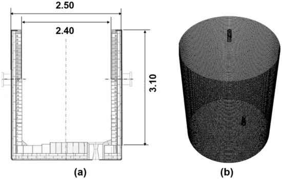
Figure 1.
(a) Geometry of the ladle furnace (m), (b) computational mesh.
The multiphase flow’s appropriate computing approach is the Eulerian scheme represented here by the Volume of Fluid Model (VOF) [14] combined with a Lagrangian model [15,16] for the dynamic trajectories of nickel particles in the melt. The model employs only one set of continuity and momentum transfer equations according to
Differential Equations (1) and (2) are solved simultaneously for the respective partial differential equations for the balances of the turbulent kinetic energy, k, and its dissipation rate, ε, embedded in the model of turbulence k-ε [17,18,19]. The contribution of turbulent stresses to the momentum equation is given by the term , in Equation (2). These differential equations solve the fluid flow velocity-field in the bulk of phase q, jump boundary conditions are applied in the interfaces. For momentum transfer, the jump-boundary condition is
The estimation of force F is through the Continuous Stress Model adopted by the ANSYS-FLUENT software [20]. To make it clear, q refers to phases liquid metal, air, and argon. The velocity is a kind of representative velocity for all phases involved in the system or what may be called the velocity of the mixture of phases. The velocity field, , is employed to solve the advection equation, which gives the volume fractions of each phase. The evolution of the volume fraction of each phase as a function of time and space and is determined by a scalar advection equation for the phases (as the sum of all volume fractions should be equal to one):
The solution procedure implies calculating the volume fraction, , which represents the fractional volume of the cell occupied by the fluid q. The unit value of represents a cell full of q, while a zero value indicates that it contains no fluid q. Cells with between 1 and 0 must contain an interface or interfaces where the jump boundary conditions are applied. The respective volume fractions weight the physical properties of each phase.
The calculation of the physical properties is through Equation (5), and consequently, the volume fractions of the phases are implicit in Equation (2). The tracking of the interfaces between phases is through solving the Equation (4) using an explicit scheme setting a Courant number of 0.5:
The second upwind discretization scheme [21], is a recommendable choice to discretize Equation (6). Besides using the 2nd upwind discretization, a piecewise linear interface method reconstructs the interfaces [16]. For the argon gas, the application of an inlet velocity boundary condition applies in the plug. The computation mesh consisted of 3,344,679 hexahedral cells with a maximum aspect ratio of 12.99, and maximum ortho-skewness of 0.631 and a minimum orthogonal quality of 0.153. During the numerical iteration process, the gradient method [20] serves to interpolate the values of the flow variables from the centroids of the cells to their faces. Figure 1b shows the computational mesh employed for the solution of the system of partial differential equations [11].
2.2. Boundary Conditions
At all solid surfaces, the bottom and wall of the ladle, and the internal wall of the EBT sleeve, there is a no-slip condition of velocity. The logarithm law function [20] relates the step velocity gradients in the boundary layer with the outer velocities. A velocity profile obeying the 1/7 law [22] implemented as a user-defined function works inside the sleeve of the EBT. From the tip of the EBT to the top of the bath, height hb, the particle velocity at its entry in the melt was calculated as , where ut is the tip’s velocity profile. Each one of velocity vectors in that profile was modified by summing , the particle’s falling velocity, and the resulting profile is the input of particle velocity in the melt surface. On the bath surface, a pressure boundary condition applies and is equal to 101,000 Pa. At the ladle bottom, in the argon plug, a velocity boundary condition was applied. This velocity was estimated from a flow rate of 400 L/min of argon and divided by the area of the porous plug in contact with the melt with a diameter of 60 mm, assuming a uniform plug flow.
2.3. Method of Solution
The segregated-finite volume method works well to solve each one of the equations of momentum and the respective equations of the turbulent kinetic energy and its dissipation rate embedded in the k-ε model of turbulence under unsteady state conditions [15,16,17]. The PISO [23] algorithm was applied, in the segregated scheme for coupling the pressure-velocity. The criterion of converging is that when the sum of residuals of all the flow variables is less than 10−4, and then the iteration comes to the end.
2.4. Particle Dynamics
2.4.1. Trajectory of Particles
The trajectories of nickel particles were simulated through the Lagrangian model [15], solving the Equation for the second law of Newton;
The term in the left-hand side is the acceleration force on the particle of mass m, the first term in the right-hand side of Equation (7) is the gravity force on the particle. The second term includes two forces; the first is the hydrostatic force due to the pressure, and the second is to the shear stress acting on the particle.
The third term in the right-hand side of Equation (7) is the drag force, where is evaluated at the local position of the particle; is particle diameter. Neglecting the Faxen force, which includes the Laplacian , the drag force, can be approximated by
The fourth term is the virtual mass force corresponding to the mass of liquid displaced by the particle’s presence. The last and fifth term is the lift force from gradients of velocity and pressure acting in the particle’s surroundings and is the vorticity. The drag coefficient CD in Equation (8), is a depending function of the relative Reynolds number, and is calculated using the model of Morsi and Alexander [24]. The trajectories, of particles are calculated using their velocities in the numerical integration of Equation (9)
2.4.2. Heat Transfer
The heat flow is transported to the particle surface, initially at a room temperature of 25 °C, by the melt’s external convective motion. The heat conduction equation analysis with external flow leads to the dimensionless numbers given in Table 3 [25]. During the shell remelting process, the metallic particle heats up close to its melting point and melts before the steel shell washes out. Hence, the resistance to heat transfer resides in the shell, and it controls the melting rate. The alloying particle is a pure metal, specifically nickel. This metal has a thermal conductivity, which is a little higher than twice that of steel, and this meets the assumption of a negligible internal thermal resistance, see Table 4, where there are thermophysical data of other metals for comparison purposes. Nickel has a melting point of 1455 °C, and melts before the steel shell, and by the time that the steel shell is liquid, so is the metallic pellet. A further assumption is to neglect the lower melting point effects of nickel on the shell’s interior wall. Hence, the melting rate is under control of the thermal response of the outer steel shell. Besides, the nickel pellet size is 0.03 m for two reasons; first, it is assumed as an averaged diameter of a metallic addition thrown in the ladle and second because it allows fixing this variable avoiding more calculations. These assumptions and considerations allow focusing exclusively on the effects of the turbulence, bath height, position of the addition in the ladle, and bath superheat on metal particle’s melting rate. A heat balance determines the maximum radius of the particle when it immerses in the bath,
Table 3.
Dimensionless numbers for heat transfer [25].
Table 4.
Physical properties of metals [13,25,27].
Using the dimensionless parameter Ph (defined in Table 3), and the dimensionless shell thickness S (S = R/R0), R is the particle radius and R0 is the original radius of the particle, in the present case 0.015 m and then, Equation (10) transforms into
The dimension Rmax-R0 is the initial thickness of the steel shell, and the time consumed by its growth is assumed to be infinitely small. The heat balance for the remelting process of a particle with very high thermal conductivity is (see nomenclature and Table 3)
The integration of Equation (12) is from R = Rmax to R = R0 in the left. Moreover, the time goes from t = 0 to t = t1 on the right side, where t1 is the melting time of the shell. Equation (12) yields in terms of dimensionless variables (see Table 3 and nomenclature):
where Bi is the Biot number, in terms of the Nusselt number is, , we get
where the dimensionless temperature is . The product is the dimensionless heat flux from the melt to the shell surface.
The calculation of the melting rate of the particle uses the local-temporal velocities of the melt-particle couple. The integration of Equation (12) using a time-location depending Nusselt number gives,
and
The Nusselt number will change with time and the specific velocity field in a given region of the melt. The Nusselt number and the local hydrodynamics conditions are linked through the particle’s local relative Reynolds number. The calculation of the Nusselt number is through the Ranz and Marshall Equation [26], given as,
where Pr is the Prandtl number and Rer the relative Reynolds number based on the difference of velocities between the melt and the particle, both calculated through the mathematical model. The instantaneous Nusselt number is substituted in Equation (15), and its numerical integration permits the estimation of the instantaneous particle’s radius.
3. Results and Discussion
3.1. Effect of Turbulence on the Nusselt Number
To visualize these results, Figure 2 divides the ladle into North N, South S, East E, and West W sectors, and the addition or falling of nickel is in the points along these axes. Figure 3a,b shows a 3D view of the particle’s trajectory, its residence time in the color scale, and the variations of the Nusselt number at a bath level of 16 tons when a nickel particle falls in point N3. The nickel particle sinks until the bottom and slides down, and after 1 s, interacts, during a short time, with the deviated argon plume, later continues its trajectory until contacting the wall, as shown in Figure 3a.
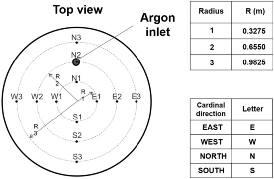
Figure 2.
Falling points of additions over the top of the bath. Each point corresponds to a vertical plane located in the N–S and E–W axes. The top table indicates the distances from the ladle center.
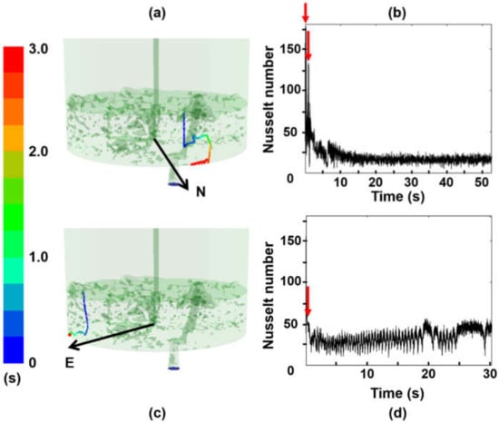
Figure 3.
Particle trajectories, residence times, and Nusselt numbers at bath level of 16 tons. (a) A 3D view of the particle trajectory in the multiphase flow, the addition is in point N3. (b) Variations of the Nusselt number with time after the particle falls in point N3. (c) A 3D view of the particle trajectory in the multiphase flow, the addition is in point E3. (d) Variations of the Nusselt number with time after the particle falls in point E3. Steel superheat is 15 K.
The green iso-surfaces seen in this figure, and in the next coming, represent the argon and air bubbles.
The plot of the Nusselt number is in Figure 3b and is sensitive to the external flow. At the particle’s immersion time, the Nusselt number is high due to the big difference between its velocity and the melt velocity yielding a large Reynolds number. The particle later interacts with the argon plume enhancing the Nusselt number; see the first arrow in Figure 3b. Just 1 s later, the local Nusselt number observed a sudden increase indicated by the second arrow, due to the interaction with the argon bubbles. The particle slides down along the bottom and reaches the corner formed by the ladle bottom and the wall. There, the Nusselt number decreases, with some up–downs due to the contact with liquid streams since the particle finds itself in a region of variable melt velocities. The trajectory of the particle falling in point E3 is shown in Figure 3c,d. In this case, the Nusselt is high at the immersion time due to the high particle entry velocity and decreases rapidly once the particle sinks until touching the ladle bottom where the melt pushes it to the corner between the bottom and the wall of the ladle. In the corner, the particle meets the air bubbles entrained by the entry jet inducing a local rise of the turbulence level, and this gives the slight increase of the Nusselt number as seen in Figure 3d.
The trajectories, residence times, and the Nusselt numbers of the sinking particle at bath levels of 30 and 50 tons are shown in Figure 4a–d when the particle falls in point N2. The addition of the particle in point N2, just above the argon plug, is not a guarantee for obtaining large Nusselt numbers at a bath level of 30 tons neither at a bath level of 50 tons. The reason is that the argon plume remains deviated at these bath levels, from the vertical and the particle sinks without direct interaction with the turbulence produced by the rising bubbles of the argon plume. Therefore, the Nusselt number observes an initial large magnitude due to the particle’s entry effects in the melt and decreases until its final melting process. Figure 5a shows the trajectory and the residence time when the particle falls in point N3 and Figure 5b shows the variations of the Nusselt number. The nickel particle sinks making a short contact with the argon plume which induces a short increase of the Nusselt number as seen in Figure 5b. Figure 5c,d shows the corresponding plots when the particle falls in point E1. The sinking particle takes contact with the argon bubbles and is partially refloated to continue sinking later towards the ladle bottom. The sensitivity of the Nusselt number to the argon bubbles is manifested by its sudden increase as seen in Figure 5d. Therefore, these plots make clear the influence of the local turbulence on the heat flux from the liquid to the nickel particle.
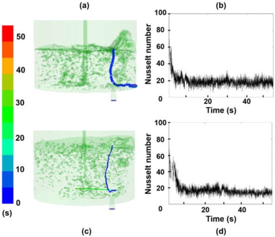
Figure 4.
Particle trajectories, residence times, and Nusselt numbers at bath level of 50 tons. (a) A 3D view of the multiphase flow at a level of 30 tons, addition point is N2. (b) Variations of the Nusselt number with time after the particle falls in point N2 at a bath level of 50 tons. (c) A 3D view of the multiphase flow at a level of 50 tons, addition point is N2. (d) Variations of the Nusselt number with time after the particle falls in point N2 at a bath level of 50 tons. Steel superheat is 15 K.
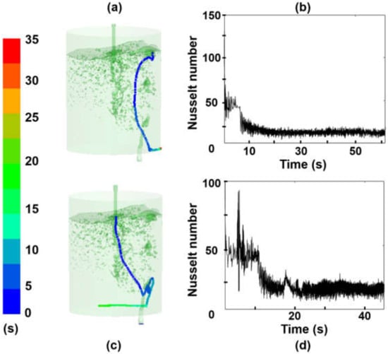
Figure 5.
Particle trajectories, residence times, and Nusselt numbers at a bath level of 80 tons. (a) A 3D view of the multiphase flow when the particle falls point N3. (b) Variations of Nusselt number with time at falling point N3. (c) A 3D view of the multiphase flow when the particle falls point E1. (d) Variations of Nusselt number with time at falling point E1.
Figure 5d is repeated as Figure 6a to make a direct comparison with the variations of the instantaneous particle’s radius vs. time shown in Figure 6b, the slope of this curve gives the melting rate. The time period marked by 1 is characterized by a sudden increase of the Nusselt number in Figure 6a results in a high melting rate of the particle as seen by the large slope of the curve in Figure 6b. As the Nusselt number decreases, after the particle abandons the argon bubbles, the melting rate decreases as seen in the time period 2.
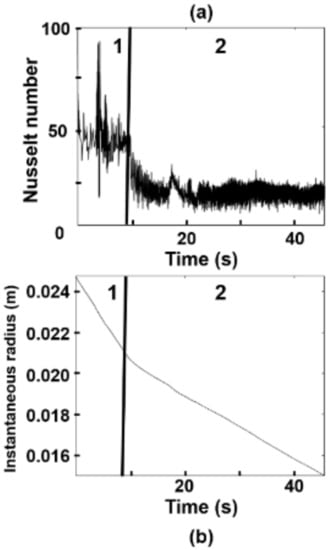
Figure 6.
Instantaneous Nusselt number and its effect on the melting rate of the shell. (a) Variations of Nusselt number with time when the particle falls in point E1. (b) Decrease of the shell thickness with time when the particle falls in point E1. Steel superheat is 15 K.
3.2. Melting Rates
The melting rates corresponding to the addition or falling points of the particle in the N–S and E–W sectors are in Figure 7a,b, respectively. At these 16 tons, the melting rates are larger in the south than in the north sector, and the addition of nickel in the points N1 and N2 yields the slowest melting rates despite the presence of the argon plume in this sector. These rates are due to the deviation of the argon plume, which avoids a direct interaction with the particle, as seen in Figure 7c. When the particle falls in points S3 and S1 the particle observes the largest melting rates in the N–S axis. The melting rates in the E–W sectors, Figure 7b, are higher in the addition points W1, W2, and W3 than in points W1, C, E1, E2, and E3. Even, the melting rates are larger in the W sector than in the S sector. These differences are derived from higher melt velocities in N–S axis than in the E–W axis, as seen by velocity fields shown in Figure 7c,d.
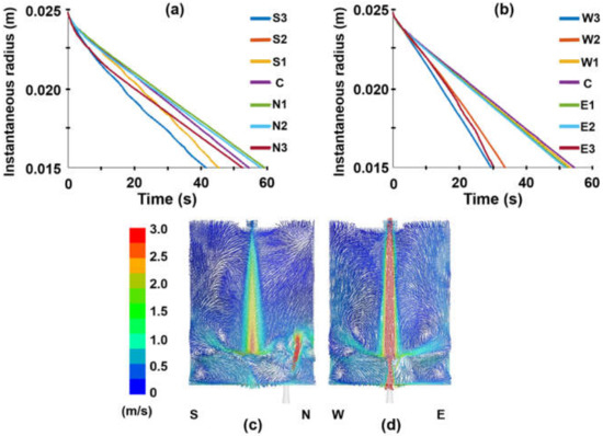
Figure 7.
Melting rate of the outer shell and velocity fields in vertical planes at a bath level of 16 tons. (a) Axis N–S, (b) Axis E–W. Steel superheat is 15 K. (c) Central plane through the argon plume, (d) central plane perpendicular to the plane passing through the argon plume. The color bar is a velocity scale.
The addition of the particle in points of the N–S axis at a bath level of 50 tons yields a broader spread of melting rates along the N–S axis, and particularly the highest melting rates reported by points N3 and S1, as seen in Figure 8a. In Figure 8b, the rest of the addition points along the axis E–W yield similar melting rates with slightly higher melting rates in points E1 and E2. The high melting rates in point N3 are originated by the region of large velocities of the liquid phase, as indicated by the arrow in Figure 8c. Indeed, the plume’s deviation toward the ladle wall raises the velocity of the liquid as is indicated by that arrow. The melting rate is relatively high when the particle falls in the point S1, since the it goes through a region of high velocities as is indicated by the corresponding arrow in a 3D view shown in Figure 8c. These velocity fields are visualized from a different perspective in the 2D view in the plane passing through the N–S axis in Figure 8d.
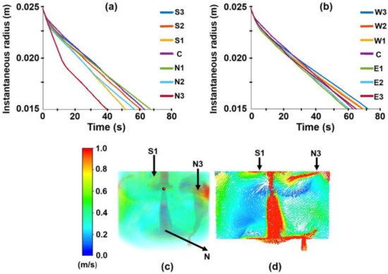
Figure 8.
Melting rate of the outer shell and velocity fields in vertical planes at a bath level of 50 tons. (a) Axis N–S, (b) Axis E–W. Steel superheat is 15 K. (c) 3D view of the velocity field. (d) Central plane perpendicular to the plane passing through the argon bubble.
At the highest steel level of 80 tons, the variety of melting rates is wider, and the highest melting rates are observed when the particle falls in points N2, above the plume spout, and S2 in the opposite side in the N–S axis where the particle falls through regions of high velocities (see Figure 9a,c,d). The slowest melting rate is observed when the particle falls in point S3. In point N2, the plume rises straightly, making possible the particle’s direct interaction with the argon plume, and when it falls in point S2 the particle passes through regions of high velocities. Both cases result in enhancing the heat flux from the melt to the particle. When the particle falls in point S3 it sinks passing through low velocities regions, resulting in slower melting rates. These physical interactions are indicated in the 3D view of Figure 9c, by the corresponding arrows. Along the E–W axis, the particle’s highest melting rate is observed in point E1 and the slowest in point W2 (see Figure 9b). The nickel particle’s sinking path passes through regions of high velocities when the particle falls in point E1 and through regions of low velocities when the particle falls in point W2 as indicated by the respective arrows in Figure 9c. Figure 9d shows a 2D view of the velocity field in a plane passing along the N–S axis and is helpful to visualize the sinking region when the particle falls in points N2, S2, and S3.
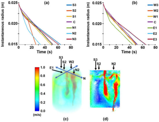
Figure 9.
Melting rate of the outer shell and velocity fields in vertical planes at a bath level of 80 tons. (a) Axis N–S, (b) Axis E–W. Steel superheat is 15 K. (c) Central plane through the argon plume, (d) central plane perpendicular to the plane passing through the argon bubble.
3.3. Melting Times
The melting rate curves’ interception in Figure 6, Figure 7, Figure 8 and Figure 9, with the horizontal axis, defines the melting time. At 16 tons, the point S3 yields the lowest melting time in the N–S axis, as shown in Figure 10a. In the E–W axis, the shortest melting time is in point W3 at the shallow melt level, as shown in Figure 10b. The melting times are, in general, shorter along the E–W axis than in the N–S axis. At 30 tons, the melting times are similar along both axes N–S and E–W, as seen in Figure 10c,d.
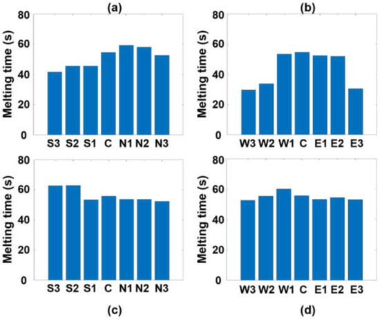
Figure 10.
Melting times of the nickel particle. (a) Additions in the N–S axis at a level of 16 tons. (b) Additions in the E–W axis at a level of 16 tons. (c) Additions in the N–S axis at a level of 30 tons. (d) Additions in the E–W axis at a level of 30 tons. Steel superheat is 15 K.
At 50 tons, the melting times become shorter for the points located in the N–S axis, as is seen in Figure 11a,b, and this condition is more defined when the level is 80 tons, as is seen in Figure 11c,d. These effects have their origin in the high levels of turbulence as Nájera-Bastida et al. [11] reported using turbulent viscosity maps; see Figures 11 and 12 of this reference, when the ladle is close to its full capacity. Therefore, tall baths generate long-vertical recirculating flows, driving the particle through high-velocity regions favoring the heat fluxes from the melt to the particle, favoring the melting rates of sinking particles in iron baths.
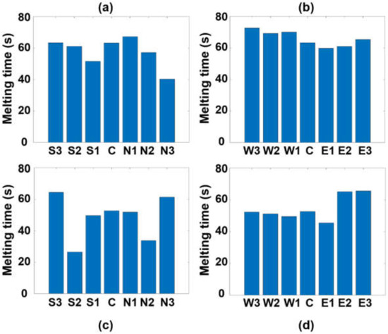
Figure 11.
Melting times of the nickel particle. (a) Additions in the N–S axis at a level of 50 tons. (b) Additions in the E–W axis at a level of 50 tons. (c) Additions in the N–S axis at a level of 80 tons. (d) Additions in the E–W axis at a level of 80 tons. Steel superheat is 15 K.
3.4. Combined Effects on the Melting Rate
Figure 12a,b summarizes the combined effects of superheat and the particle’s falling position on its melting time for the lowest ladle level of 16 tons for the N–S and E–W axis, respectively. Figure 12c,d shows the plots corresponding to the ladle levels of 50 tons for the N–S and E–W axis. At higher superheats, larger than 50 K, the melting time becomes slightly dependent on the particle’s falling point. The melting times are more dependent on the falling position of the nickel particle at low superheats.
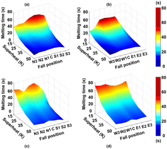
Figure 12.
Effects of melt superheat and position of the particle addition on the melting time of the shell. (a) N–S axis at bath level of 16 tons. (b) E–W axis at a bath level of 16 tons. (c) N–S axis at bath level of 50 tons. (d) E–W axis at bath level of 50 tons.
3.5. Practical Implications
Heavy additions observe the tendency to sink fast until the ladle bottom. These additions should fall in shallow baths on the opposite side of the argon plug for the fast alloying purpose. Fast melting is also possible if the particle falls just above argon plume at high steel levels in the ladle. Melting rates are less dependent on hydrodynamics when the superheats are higher. These types of additions are already melted and mixed at the time that the tapping ends.
4. Conclusions
The present research focused on the melting times of sinking high-melting point additions affected by the fluid dynamics of liquid steel during the tapping operation with simultaneous ladle bottom argon stirring. The results of the numerical results lead to the following conclusions.
- The heat transfer coefficient is a function of the time and local coordinates of the particle trajectory. Therefore, the melting rate of particles, for a given superheat, is dependent on the local position of a particle and steel level in the ladle.
- Due to the local turbulence levels, the melting rate of a particle increases when its trajectory crosses through high turbulent fields and decreases when it goes through low turbulence.
- The melting rates of a particle are dependent on the bath level of steel tonnage in the ladle. At low bath levels, the melting rates are higher in the opposite side where the argon plume is due to its deviation driven by the impacting streams of liquid steel in the ladle bottom.
- At high ladle levels, a particle’s melting rates are higher in the side where the argon plume is since it rises straightly, allowing more direct interaction and larger heat fluxes.
- Particles fed on the opposite side can melt fast if they sink through a field of small velocities, and are dragged to the argon bubbling region in the ladle bottom. At higher superheats, particles’ melting times become less dependent on the fluid flow dynamics of liquid steel.
Author Contributions
Conceptualization: R.M.-D., Methodology: R.M.-D. and A.N.-B., Software: J.R.-Á., C.R.M.-V., Formal analysis; R.M.-D. and A.N.-B., Investigation; R.M.-D., Supervision: R.M.-D. and K.C. All authors have read and agreed to the published version of the manuscript.
Funding
This research was funded by Consejo Nacional de Ciencia y Tecnología (CoNaCyT), SNI, and University of Toronto.
Acknowledgments
The authors give the thanks to the institutions IPN, University of Toronto, SNI, and CoNaCyT for their support to the Process Engineering Groups.
Conflicts of Interest
The authors declare no conflict of interest.
Nomenclature
| A | cross-section area of the metallic particle in the bath |
| CP | heat capacity |
| D | diameter |
| g | gravity constant |
| ΔH | enthalpy |
| h | height and heat transfer coefficient hp of the particle |
| curvature radius | |
| thermal conductivity, kinetic energy | |
| m | mass |
| n | normal vector |
| p | pressure |
| q | heat flux and phase q |
| R | particle radius |
| ratio of physical properties like CP, k, α | |
| trajectory of the particle | |
| S | dimensionless shell thickness |
| T | temperature |
| t | time |
| . | averaged velocity of the mixture |
| volume | |
| v | particle velocity |
| Greek Symbols | |
| α | thermal diffusivity |
| δ | thickness of the boundary layer |
| tensor of Levy–Civita | |
| dissipation rate of kinetic energy | |
| Ω | dimensionless number, Equation (16) |
| ωij | vorticity |
| Π | total stress |
| χ | phase indicator |
| µ | viscosity |
| density | |
| τ | stress |
| ratio of thicknesses | |
| Θ | dimensionless temperature |
| Sub-Indexes | |
| B | boundary |
| I | interface |
| L | liquid |
| M | metal |
| m | mean average |
| max | maximum value |
| p | particle |
| q | phase q |
| 0 | initial value of the nickel particle´s radius |
| rms | root mean square |
| i, j, k | are indexes for coordinates. When only one index i used, that means the three directions. |
References
- Carreño-Galindo, V.; Morales, R.D.; Serrano, J.A.; Chavez, J.F. Thermodynamics analysis of steel deoxidation processes during tapping and refining operations. In Proceedings of the 57th Electric Arc Furnace Conference, Iron and Steel Society, Pittsburgh, PA, USA, 14–16 November 1999; pp. 523–534. [Google Scholar]
- Argyropoulos, S.A.; Guthrie, R.I.L. The dissolution of titanium in liquid steel. Metall. Mater. Trans. B 1984, 15, 47–58. [Google Scholar] [CrossRef]
- Pandelaers, L.; Verhaeghe, F.; Blanplain, B.; Wollants, P.; Gardin, P. Interfacial reactions during titanium dissolution in liquid iron: A combined experimental and modeling approach. Metall. Mater. Trans. B 2009, 40, 676–684. [Google Scholar] [CrossRef]
- Guthrie, R.I.L.; Clift, R.; Henein, H. Contacting problems associated with aluminum and ferro-alloy additions in steelmaking-hydrodynamics. Metall. Mater. Trans. B 1975, 6, 321–329. [Google Scholar] [CrossRef]
- Tanaka, M.; Mazumdar, D.; Guthrie, R.I.L. Motions of alloying additions during furnace tapping in steelmaking processing operations. Metall. Mater. Trans. B 1993, 24, 639–648. [Google Scholar] [CrossRef]
- Rodríguez-Ávila, J.; Morales, R.D.; Nájera-Bastida, A. Numerical study of multiphase flow dynamics of plugging jets in liquid steel and trajectories of ferroalloy additions in a ladle during tapping operations. ISIJ Int. 2012, 52, 814–822. [Google Scholar] [CrossRef]
- Berg, H.; Laux, H.; Johanssen, S.T. Flow pattern and alloy dissolution during tapping of steel furnaces. Ironmak. Steelmak. 1999, 26, 127–139. [Google Scholar] [CrossRef]
- Reza Aboutalebi, M.; Vadhati Khaki, J. Heat transfer modelling of the melting of solid particles in an agitated molten metal bath. Can. Metall. Quart. 1998, 37, 305–311. [Google Scholar] [CrossRef]
- Duan, H.; Zhang, L.; Thomas, B.G.; Conejo, A. Fluid flow, dissolution, and mixing phenomena in argon-stirred steel ladles. Metall. Mater. Trans. B 2018, 49, 2722–2743. [Google Scholar] [CrossRef]
- Webber, D.S. Alloy Dissolution in Argon Stirred Steel. Ph.D. Thesis, Metallurgical Engineering, Missouri University of Science and Technology, Rolla, MO, USA, 2011. [Google Scholar]
- Nájera-Bastida, A.; Rodríguez-Ávila, J.; Guarneros-Guarneros, J.; Morales, R.D.; Chattopadhyay, K. Changes of Multiphase Flow Patterns during Steel Tapping with Simultaneous Argon Bottom Stirring in the Ladle. Metals 2020, 10, 1036. [Google Scholar] [CrossRef]
- Water - Physical Properties. Available online: https://www.britannica.com/science/water/Physical-properties (accessed on 10 April 2019).
- Kubaschewski, O.; Alcock, C.B. Metallurgical Thermochemistry, 5th ed.; Oxford-Pergamon: London, UK, 1979; p. 349. [Google Scholar]
- Hirt, C.W.; Nichols, B.D. Volume of fluid (VOF) method for the dynamics of free boundaries. Comp. Physics 1981, 39, 201–225. [Google Scholar] [CrossRef]
- Crowe, C.T.; Schwarzkopf, J.D.; Sommerfeld, M.; Tsuji, M. Multiphase Flow with Droplets and Particles, 2nd ed.; CRC Press: New York, NY, USA, 2012; p. 68. [Google Scholar]
- Yeoh, G.H. Computational Techniques for Multiphase-Flows; Butterworth-Heinemann, Oxford: London, UK, 2010; p. 215. [Google Scholar]
- Wilcox, D.C. Turbulence Modeling for CFD; DCW Industries: La Cañada, CA, USA, 2000; pp. 103–104. [Google Scholar]
- Chung, T.J. Computational Fluid Dynamics; Cambridge University Press: London, UK, 2002; pp. 218–220. [Google Scholar]
- Pope, S. Turbulent Flows; Cambridge University Press, Cambridge Press: London, UK, 2000; p. 373. [Google Scholar]
- ANSYS, Inc. Available online: www.ansys.com (accessed on 10 April 2019).
- Ferziger, H.; Peric, M. Computational Methods for Fluid Dynamics; Springer: New York, NY, USA, 2002; p. 72. [Google Scholar]
- Bird, R.B.; Stewart, W.E.; Lightfoot, E.N. Transport Phenomena; Wiley International: Hoboken, NJ, USA, 1960; p. 153. [Google Scholar]
- Issa, R.I. Solution of the implicitly discretized fluid flow equations by operator-splitting. Comp. Physics 1986, 62, 40–65. [Google Scholar] [CrossRef]
- Morsi, A.J.; Alexander, S.A. An investigation of particle trajectories in two-phase flow system. J. Fluid Mech. 1972, 55, 193–208. [Google Scholar] [CrossRef]
- Zhang, L.; Oeters, F. Melting and Mixing of Alloying Agents in Steel Melts; Verlag Stahleissen GmbH: Dusseldorf, Germany, 2006; p. 1. [Google Scholar]
- Ranz, W.E.; Marshall, W.R. Evaporation from drops: Part II. Chem. Eng. Prog. 1952, 48, 173–180. [Google Scholar]
- Nordberg, M.; Nordberg, G.F.; Fowler, B.A. Handbook on the Toxicology of Metals; Elsevier-Academic Press: Amsterdam, The Netherlands, 2011; p. 743. [Google Scholar]
© 2020 by the authors. Licensee MDPI, Basel, Switzerland. This article is an open access article distributed under the terms and conditions of the Creative Commons Attribution (CC BY) license (http://creativecommons.org/licenses/by/4.0/).