Abstract
Distributed constraint satisfaction problems (DisCSPs) are among the widely endeavored problems using agent-based simulation. Fernandez et al. formulated sensor and mobile tracking problem as a DisCSP, known as SensorDCSP In this paper, we adopt a customized ERE (environment, reactive rules and entities) algorithm for the SensorDCSP, which is otherwise proven as a computationally intractable problem. An amalgamation of the autonomy-oriented computing (AOC)-based algorithm (ERE) and genetic algorithm (GA) provides an early solution of the modeled DisCSP. Incorporation of GA into ERE facilitates auto-tuning of the simulation parameters, thereby leading to an early solution of constraint satisfaction. This study further contributes towards a model, built up in the NetLogo simulation environment, to infer the efficacy of the proposed approach.
1. Introduction
Agent-based simulations are widely employed to address computationally hard problems in a distributed context. These problems are either innately distributed in nature [1] or formulated as an instance of distributed constraint satisfaction problems (DisCSPs). In the past, different algorithms have been proposed to model diversified computationally intractable problems in the context of DisCSP. Most notably among them is the pioneering work of Yokoo et al. [2,3,4], further improved upon by Silaghi et al. [5,6,7].
The identification of the set of variables and imposed constraints is imperative to represent the problem as a constraint satisfaction problem (CSP) (Definition 1). Each constraint pertains to some subset of variables and limits the permitted combinations of variable values in the subset. Solving a CSP requires identifying one such assignment of variables that meet all constraints. In some cases, the aim is to obtain all sets of such assignments. However, finding the number of all possible solutions to a given CSP is also equally hard and proven to an NP-complete problem [8].
A distributed CSP is a CSP with the variables and constraints distributed among multiple agents (Definition 3) [9].
The ERE (environment, reactive rules and entities) algorithm is an autonomy-oriented computing (AOC)-based algorithm that manifests several inherent distinctive characteristics of autonomous systems, which make it advantageous to solve problems involving large-scale, greatly dispersed, regionally interacting and occasionally uncertain entities [10]. The ERE algorithm is a practical approach to searching for both accurate and approximate solutions to a CSP in the reduced number of execution steps. Such a reduction enables the ERE algorithm to exhibit promising results when used for solving benchmark problems, like n-queen problems, uniform random-3-SAT (Satisfiability) problems and flat graph coloring problems [10].
Fernandez et al. [11] formulated a wireless sensor tracking system as an instance of DisCSP, known as SensorDCSP and profoundly investigated in this exposition. In this study, we use a combination of genetic algorithm (GA) and the ERE algorithm for the SensorDCSP problem to achieve optimum visibility and compatibility between sensors and mobiles. Consolidation of GA into ERE, auto-tune simulation parameters resulted in the ameliorated model yielding the optimal solution.
AOC by self-discovery is the other closely-related concept of tuning parameters, wherein simple rules are used to adjust the parameters of an autonomous system [12].
2. Related Work
Problems from diverse application domains are modeled as DisCSP. Potential DisCSPs are the problems dealing with the decision of a consistent combination of agent actions and decisions. Typical examples include distributed scheduling [13], distributed interpretation problems [14], multiagent truth maintenance systems (a distributed version of a truth maintenance system) [15,16] and distributed resource allocation problems in a communication network [17]. Owing to the conceptualization of a large number of distributed artificial intelligence (DAI) problems as DisCSPs, algorithms for solving DisCSP play a vital role in the development of DAI infrastructure [18].
2.1. Constraint Satisfaction Problem and Its Variations
Definition 1.
CSP is a triple,< x, D, C > consisting of n variables x = x1, . . . ., xn; the values of these variables are derived from finite, discrete domains D = {D1, . . . ., Dn}, respectively, and C = {C1, . . . ., Cn} is a set of constraints on their values. Every constraint Ci ∈ C can be represented as a pair < tj, Rj >, where Rj is a k-ary relation on the corresponding subset of domains dj, and tj ⊂ x is a subset of k variables. That is, the constraint pk (xk1, . . . .xkj) is a predicate that is defined on the Cartesian product Dk1 × ... × Dkj [19].
Definition 2.
An evaluation of the variables is known as a function from a subset of variables to a particular set of values in the corresponding subset of domains. An evaluation is said to be satisfying a constraint < tj, Rj > if the relation Rj is satisfied for values assigned to the variables tj. If an evaluation does not violate any of the constraints, it is said to be consistent. If an evaluation includes all variables (i.e., k=n), then it is said to be complete. An evaluation is a solution if it satisfies all constraints and includes all variables; such an evaluation is said to solve the constraint satisfaction problem [20].
Definition 3.
DisCSP is a CSP in which variables and constraints remain distributed among multiple agents. In the algorithms used to solve DisCSP, the agents are treated as autonomous solvers for finding partial solutions for the problem at hand [9].
2.2. SensorDSCP
Motivated by the real distributed resource allocation problem, Fernandez et al. [11] proposed the distributed sensor-mobile problem (SensorDCSP). It consists of a set of sensors s1, s2... sn and a set of mobiles m1, m2... mq.
In SensorDCSP, a sensor can monitor at the most one mobile, and three sensors must monitor a mobile. An assignment of three distinct sensors to each mobile is a valid solution following two sets of constraints, i.e., visibility and compatibility. A directed arc between mobiles indicates the visibility of mobiles to a sensor in the visibility graph. An arc in the compatibility graph between two sensors represents the compatibility between them (Figure 1). In the solution, the three sensors assigned to each mobile are the sensors that form a triangle where the mobile is inside. This sensor-mobile problem is NP-complete [11] and can be easily reduced to the problem of partitioning a graph into cliques of size three, which is a well-known NP-complete problem [21].
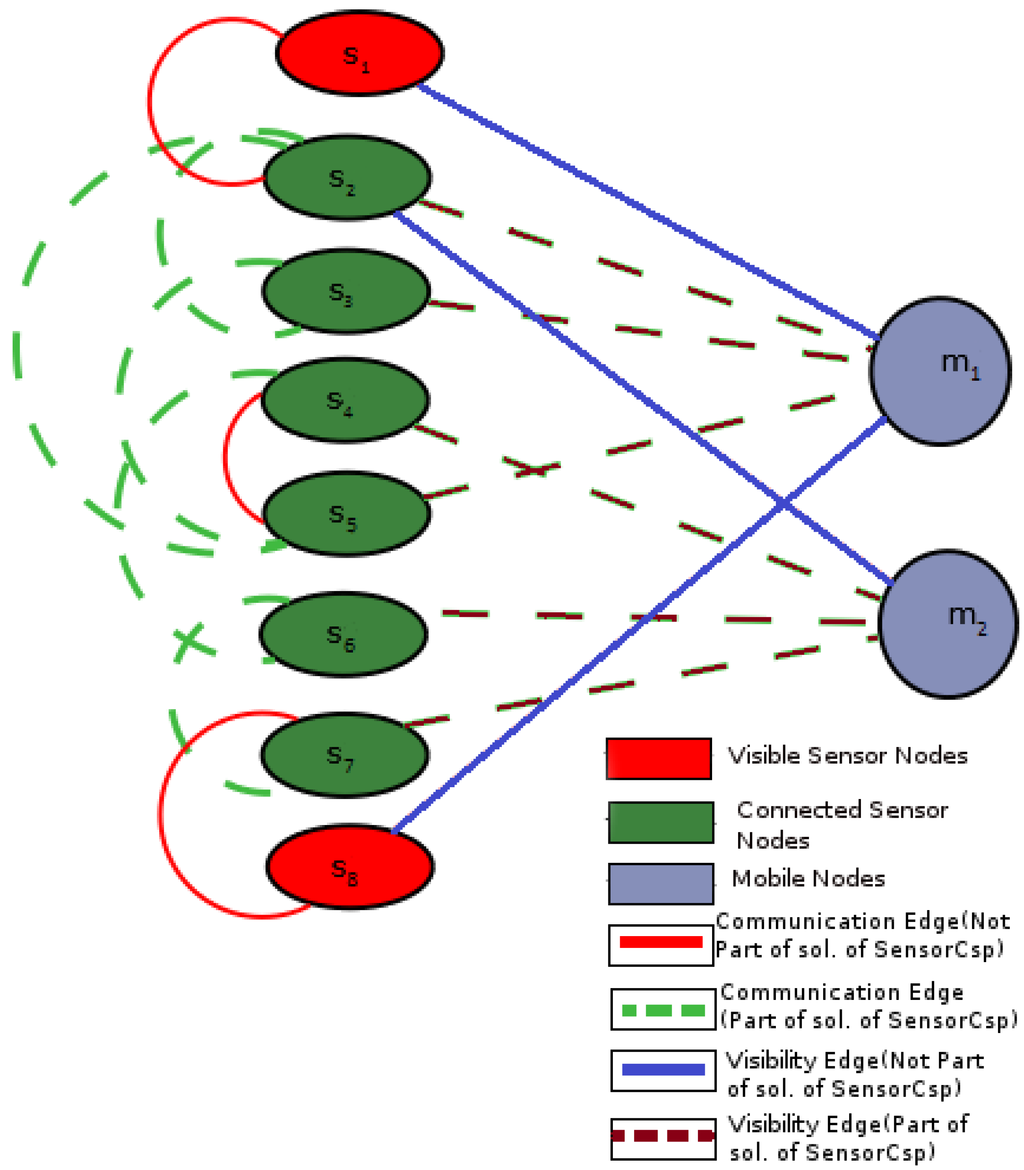
Figure 1.
An example Graph G with communication and visibility edges between the sensor and mobile nodes: dashed edges represent a solution to SensorCSP (CSP, constraint satisfaction problem) in this graph (adapted from Bejar et al. [22]).
2.3. Environment, Reactive Rules and Entities Algorithm
The ERE method achieves a notable minimization in the overhead communication cost in comparison to the DisCSP algorithms proposed by Yokoo et al [3]. This method implements entity-to-entity communication, wherein each entity is notified of the values from other relevant entities by retrieving an n × n look-up memory table instead of a pairwise value swapping. The succeeding discussion about the ERE algorithm is based on the pioneering work of Liu et al. [10]
Figure 2 elucidates the movement of entities in the environment. The grid represents an environment, where each row represents the domain of a sensor node, that is the mobile node, which it can track, and the length of the row is equal to the total number of mobile nodes in the wireless network. In each row, there exists only one entity or sensor, and each entity will move within its respective row. There are n sensors and q mobile nodes denoted by si and mj, respectively. The movement of each entity si will be within its respective row. At each step, the positions of entities provide an assignment to all sensors, whether it is consistent or not. Entities attempt to find better positions that can lead them to a solution state.
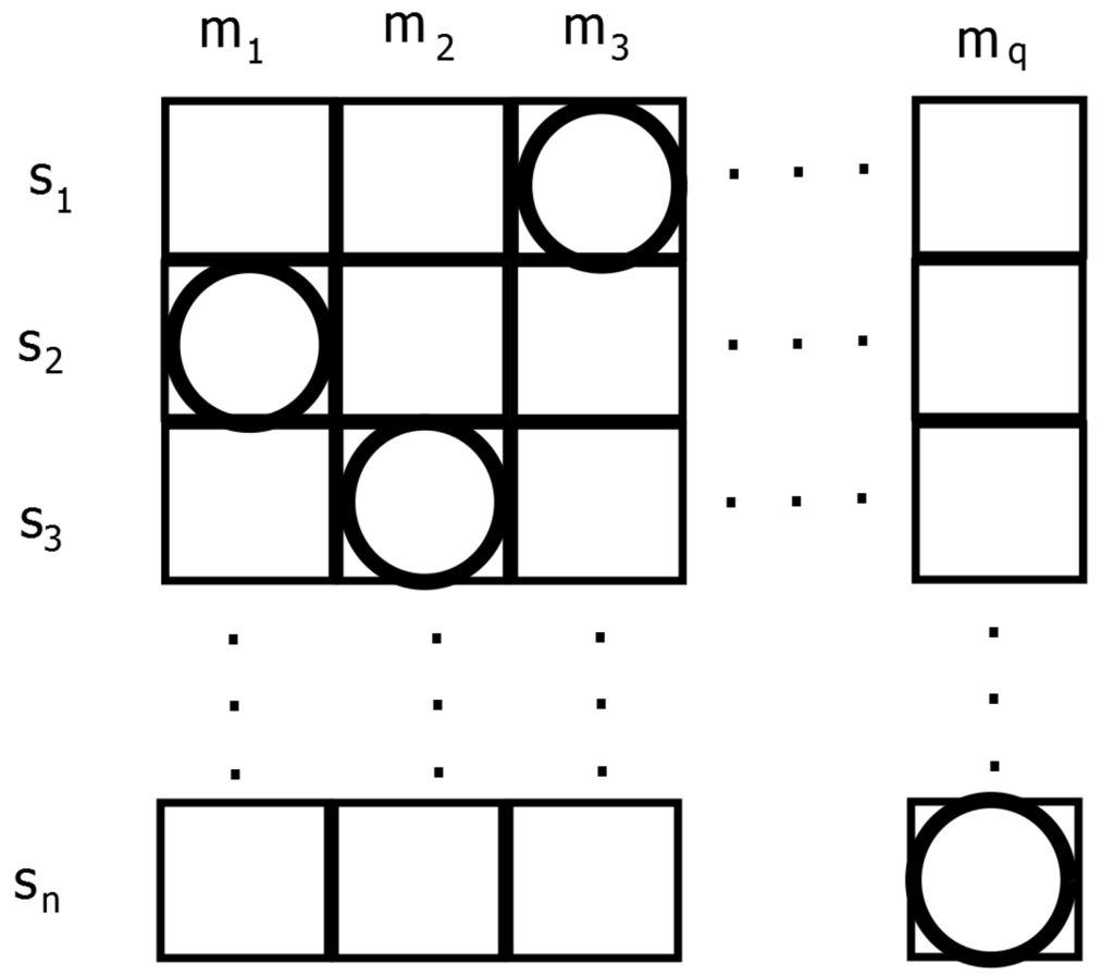
Figure 2.
An illustration of the environment, reactive rules and entities (ERE) model used (Adapted from Liu et al. [10]).
In any state of the ERE system, the positions of all entities indicate an assignment to all sensors (Figure 2). The three rudimentary behaviors exhibited by the ERE algorithm are; least move, random move and better move. It is easier for an entity to find a better position by use of a least move, since a least move checks all of the positions within a row in the table, while a better move randomly selects and checks only one position. This results in the following conundrum:
Many entities cannot find a better position to move at each step, hence if all entities use only random move and better move behaviors, the efficiency of the system will be moderate. On the other hand, a better move has lesser time complexity compared to that of a least move. Thus, a neutral point between a least move and a better move is highly recommended to improve the performance of the system under consideration (Figure 3).
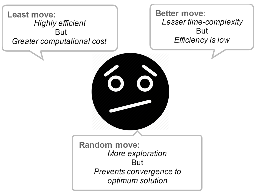
Figure 3.
An illustration of different moves in the ERE model.
To maintain a balance between least-moves and better-moves , an entity will make a better move to compute its new position. If it succeeds, the entity will move to a new position. However, if it fails, it will continue to perform some further better-moves until it finds a satisfactory better move. If it fails to take all better-moves, it will then perform a least move. More better-moves increase the execution time, and fewer better-moves cannot provide enough chance for entities to find better positions. Therefore, in the beginning, either a random move or a least move is probabilistically selected by the entity, because opting for a least move will give more chances to select a better move before a least move to maintain the desired system performance [10].
Following are the three primitive behaviors of entities to accomplish a movement:
Remark 1.
Least move: An entity moves to a minimum-position with a probability of least − p . If there exists more than one minimum position, the entity chooses the first one on the left of the row.
Remark 2.
Better move: An entity moves to a position with a probability of better − p resulting in the smaller violation value than its current position. To achieve this entity, randomly select a position and compare its violation value with the violation value of its current position, and decide accordingly. ψb defines the behavior of a better move behavior as follows:
where r is a random number generated between one and k.
Remark 3.
Random move: An entity moves randomly with a probability of random − p that is smaller than the probabilities of choosing least move and better move. Making a least move and better move alone will leave the entity in the state of local optima, thereby preventing it from moving to a new position.
The ERE method has the following fundamental merits compared to other methodologies prevalent in agent-based systems:
(1) The ERE method does not necessitate any procedure for preserving or dispensing consistent partial solutions as in an asynchronous weak-commitment search algorithm or asynchronous backtracking algorithm [3,4]. The latter two algorithms intend to abandon a partial solution, in the case of the non-existence of any value for a variable.
(2) The ERE method is intended to obtain an approximate solution with efficiency, which proves to be useful in the exact solution search within a limited time. On the other hand, the asynchronous weak-commitment search and asynchronous backtracking algorithms are formulated with the aim of completeness.
(3) The functioning of ERE is similar to cellular automata [23,24]. There exists a similarity between the behavior exhibited by entities corresponding to the underlying behavioral rules in ERE and the sequential approach followed by local search, yet another popular method for solving large-scale CSPs [25].
2.4. Model Construction
SensorDCSP can be expressed as an example of DisCSP, wherein each agent represents one mobile and includes three variables, one for each sensor that is required to track the corresponding mobile (Table 1). The domain of a variable is the set of compatible sensors. A binary constraint exists between each pair of variables in the same agent. The intra-constraints ensure that different, but compatible sensors are assigned to a mobile, whereas inter-constraints ensure that every sensor is chosen by at most one agent.
In the model, we simulate sensors as entities (S = s1, s2, s3. . . sn), where n = number of sensors and mobiles (M = m1, m2, m3. . . mq), where q = number of mobiles as variables with the following constraints:
- (1)
- For each sensor node si, there is a tracking mobile node mj; the mobile node mj in si, where zi denotes the set of mobile nodes within the range of si.
- (2)
- Let N be the set of all sensor nodes tracking a mobile, and then, all nodes present in N must be compatible with each other.
- (3)
- Each mobile must be tracked with exactly k sensor nodes within its range. k is an input parameter to the model and may vary depending on the network.
The multi-entity system used is inherently discrete in regards to its space, time and state space. A discrete timer is used in the system for synchronization of its operations. At the start, the network is simulated, assigning positions to sensor and mobile nodes and their corresponding range. Execution of the ERE algorithm to simulate SensorDSCP begins with the placement of nsensor nodes onto the environment, s1 in row1, s2 in row2...., sn in rown. The arrangement of entities takes place in randomly selected areas, thereby supporting the generation of a random network of sensors and mobiles. Subsequently, the developed autonomous system begins execution. At each iteration, all sensors are given an opportunity to determine their movements, i.e., if or not to move and where to move. Each sensor decides which mobile node to track.
2.5. Termination
After the movements of sensors to decide their tracking mobile node, the system will check whether or not all of the sensors are at zero positions, i.e., where no constraints are violated. The sensor si can detect the local environment of rowi and identify the violation value (unsatisfied constraints) of each cell in rowi. All sensors at the zero position refer to zero unsatisfied constraints, whereby a solution state has been reached. The algorithm will terminate and thus output the obtained solution. Otherwise, the autonomous system will continue to dispatch sensor entities to move in the dispatching order. (Figure 4) demonstrates the execution steps of the proposed algorithm.
| Algorithm 1: Pseudocode of the adopted ERE algorithm [10] |
| iteration=0; |
| Assign the entities’, namely sensor and mobile nodes, initial positions. ; |
| Assign mobile node positions and violation values pertaining to sensor position and the monitored mobile; |
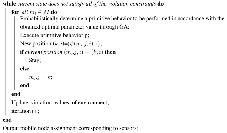 |

Table 1.
Mapping of SensorDSCP as DisCSP (distributed CSP).
| DCSP Model | Sensor-Centered Approach |
|---|---|
| Agents | Sensors |
| Variables | Mobiles |
| Intra-agent | Only one mobile per sensor |
| Inter-agent | k communicating sensors per mobile |
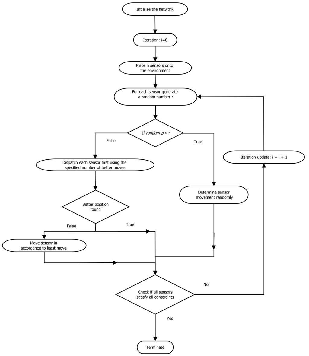
Figure 4.
Flow diagram of the algorithm.
3. Material and Methods
In this study, we utilize the combination of the above primitives to simulate the created network of SensorDSCP. It continues as follows:
(1) In the first step, the entity will probabilistically decide a behavior to execute, i.e., either random move or least move.
(2) If a least move behavior is chosen by an entity, it will have specified chances to select a better move before executing a least move. Therefore, the combination of better move and least move has the same probability as a single least move.
The values of the least − p and random − p probabilities play an important role in driving the system towards the goal. The dispatching of the entities is one after the other and does not influence the performance of the system.
3.1. Optimization Using Genetic Algorithm
Evolutionary processes in a variety of ecologically-complex systems, such as ant colonies, African wild dogs and fishes, have been known to shape group organization and logical relations within the members for some desired benefit (optimization) [26]. A large number of bio-inspired optimization algorithms have been proposed to exploit this process of evolution. The genetic algorithm (GA) is a typical example of such algorithms, which is also used within other methods to optimize the control parameters. Such hybrid techniques have reported improved performance in comparison to the technique examined in isolation. In the past, genetic algorithms have been favorably applied in the optimization of the neural networks performance by adjusting the neural weights, their topologies and learning rules. Other notable usage includes the optimization of control parameters of ant colony optimization algorithms and in the automating of the learning of fuzzy control rules by Belew et al. [27].
Pertaining to the study presented here, random move forms an essential part of the defined autonomous system, as it prevents the system from getting stuck in local optima.
3.1.1. Structure of a Chromosome
As is evident from Section 2.3, a similar probability is shared by a single least move compared to the probability of a combination of better move and least move will have. Therefore, the relevant probability is random−p (and least−p = 1-random−p). A greater random−p will, however, increase the probability of searching more areas in the search space. However, at the same time, it may prevent the population from converging to an optimum solution. A small mutation rate may lead to premature convergence, resulting in a local optimum. In light of the above, the setting of the above two parameters is a key factor in the determination of the search performance of the algorithm.
Our implementation of the genetic algorithm strives to optimize the above, the two variables for a given network instance problem. Therefore, the chromosome is comprised of the two variables: the number of better-moves before a least move and the probability of a random move (Figure 5).
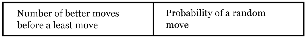
Figure 5.
Structure of the chromosome.
3.1.2. Parameters Used in the Developed Model
We developed a model in NetLogo [28] to simulate SensorDSCP using the proposed approach. The network generated is a random graph of sensors and mobiles (Figure 6). In the implementation, we use Mersenne twister, a pseudo-random number generator to assign random positions to the sensors and mobiles at the beginning of the execution of the model [29] (Figure 7). Here, we assume that all sensors are compatible with each other to simplify the network model. Table 2 describes the characteristics of the network model generated.
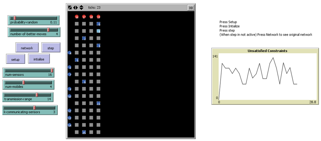
Figure 6.
Snapshot of the model running the ERE algorithm.
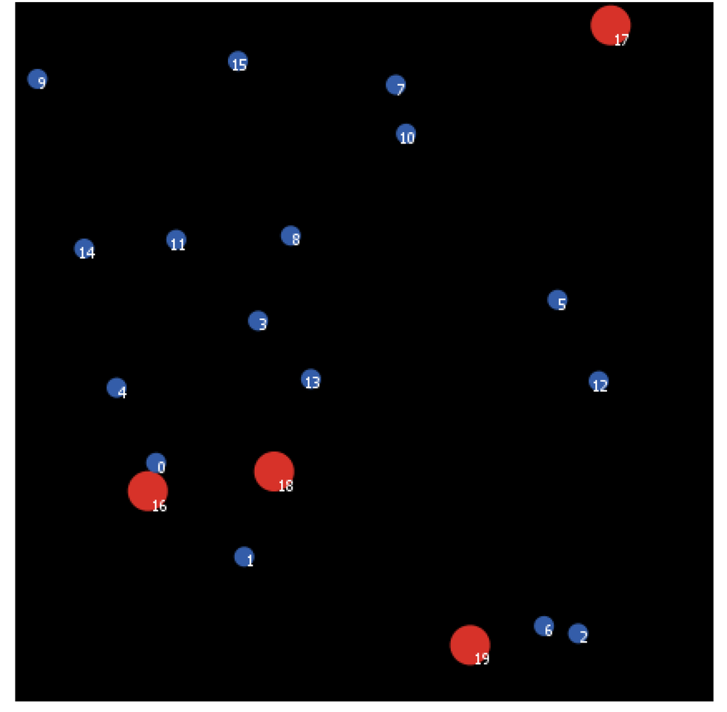
Figure 7.
Mobile sensor network generated: red nodes are mobiles, whereas blue nodes are sensor nodes.
Table 2.
Characteristics of the network model generated.
| Parameter | Value |
|---|---|
| Number of Mobile Nodes (q) | 4 |
| Number of Sensor Nodes (n) | 23 |
| Transmission Range | 3.096 cm |
| No. of Communicating Sensors Required (k) | 3 |
We apply GA to determine the optimal values of the number of better-moves before a least move and the probability of a random move for a generated network. While using GA, the minimization of the algorithm execution time with no unsatisfied constraints is the objective function. Each iteration of the usage of GA is comprised of the simulation of a given network with the parameters of ERE algorithm as the input. To avoid the non-feasible (either not yielding to the solution or taking indefinite time) values of input parameters, we restrict the implementation of the algorithm to 1000 time steps. In the model developed, this was accomplished by integrating NetLogo with R [30] and then using the GA package in R for tuning the parameters.
Table 3 describes the values of the parameters used in the implementation of GA:
Table 3.
Parameters of the genetic algorithm used.
| Parameter | Value |
|---|---|
| Population Size | 20 |
| Mutation Probability | 0.1 |
| Crossover Probability | 0.8 |
| Maximum Generations | 100 |
| Elitism | 1 |
4. Results and Discussion
In this section, we confer about the experimental results obtained by applying the proposed approach. For all implementations, we use a personal computer with 2.10 GHZ of CPU and 4 GB of RAM using NetLogo 5.1.0 [28] and R 3.1.2 [31].
4.1. Variation of the Constraints Violated
Figure 8 illustrates the variation of the constraints violated in an implementation of the ERE algorithm for a parameter setting. Here, we randomly assign values to the number of better-moves before a least move and the probability of a random move using a pseudo-random number generator [29]. One may observe that the value of the objective function does not consistently decrease to convergence. The number of constraints violated changes abruptly as the execution of the algorithm proceeds, and we cannot satisfactorily define the behavior of the complex system (SensorDSCP).
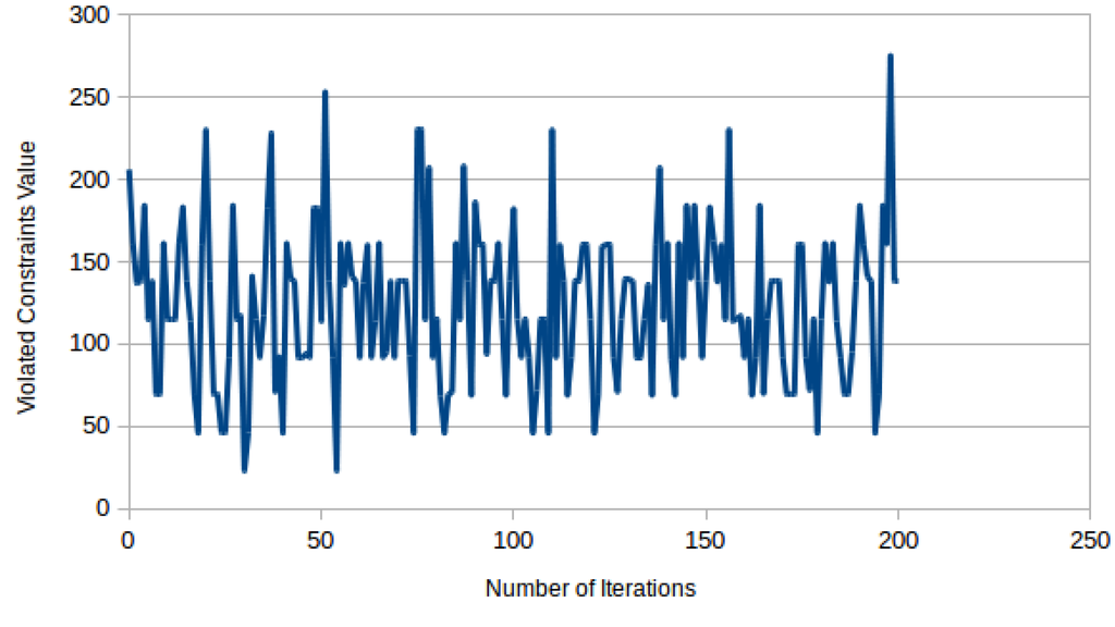
Figure 8.
Violated constraint values vs. iterations runs.
4.2. Implementation of the Genetic Algorithm for Parameter Optimization
Table 4 shows the seven different instances of the networks generated. We determine the optimal value of each of the parameters using GA. Different values of execution time (in seconds) of the algorithm leading to a solution with all constraints satisfied are also shown in the table. Here, we clearly observe that the probability of a random move gradually ceases with increasing the number of better-moves. There is an innate randomness associated with a better move that yields the system with an exploration ability, to some extent. In addition, the number of better-moves depends on the generated network and cannot be generalized for all problem instances [10]. The probability of a random move consistently reveals a value lower than 0.7 for the studied SensorDCSP instances. This not only prevents the system from getting caught in local optima, but also reduces the disruptive effects of large probability in such a parameter setting. Furthermore, a low probability of a random move also ensures the shielding of optimal solutions generated in the process.
Table 4.
Optimal values for different instances of generated networks.
| Serial No. | Number of Better-Moves | Probability of Random Move | Time (s) |
|---|---|---|---|
| 1 | 2 | 0.01211132 | 1.067 |
| 2 | 4 | 0.01194915 | 0.148 |
| 3 | 3 | 0.01227836 | 0.206 |
| 4 | 1 | 0.03812959 | 0.294 |
| 5 | 3 | 0.01582020 | 0.235 |
| 6 | 2 | 0.06199995 | 0.372 |
| 7 | 5 | 0.04419600 | 0.277 |
4.3. Comparison of the Performance of the ERE System with Genetically-Determined Parameters
Figure 9 illustrates the variation of the unsatisfied constraints for the seven different instances compared to a randomly-generated parameter setting for the ERE system. This comparison is carried out in the instances using a pseudo-random generator [29] to set the system parameters with those that are determined using GA. During experimentation, we limit the number of the iterations to 200 for the sake of a lucid visual comparison. It is clearly evident (Figure 9) that across all of the instances considered, a genetically-optimized ERE system tends to achieve an early optimal solution compared to a randomly-parametrized ERE system. In addition, in a randomly-parametrized ERE system, not even all of the constraints are satisfied with the defined limit of generations. Additionally, in the genetically-optimized ERE system, a generation adapts from the variation in the overall unsatisfied constraints of previous generations in each successive iteration, so that it does not get trapped in local optima. A progressive improvement in the solutions for various SensorDCSP network instances with consecutive iterations can be observed appreciably.
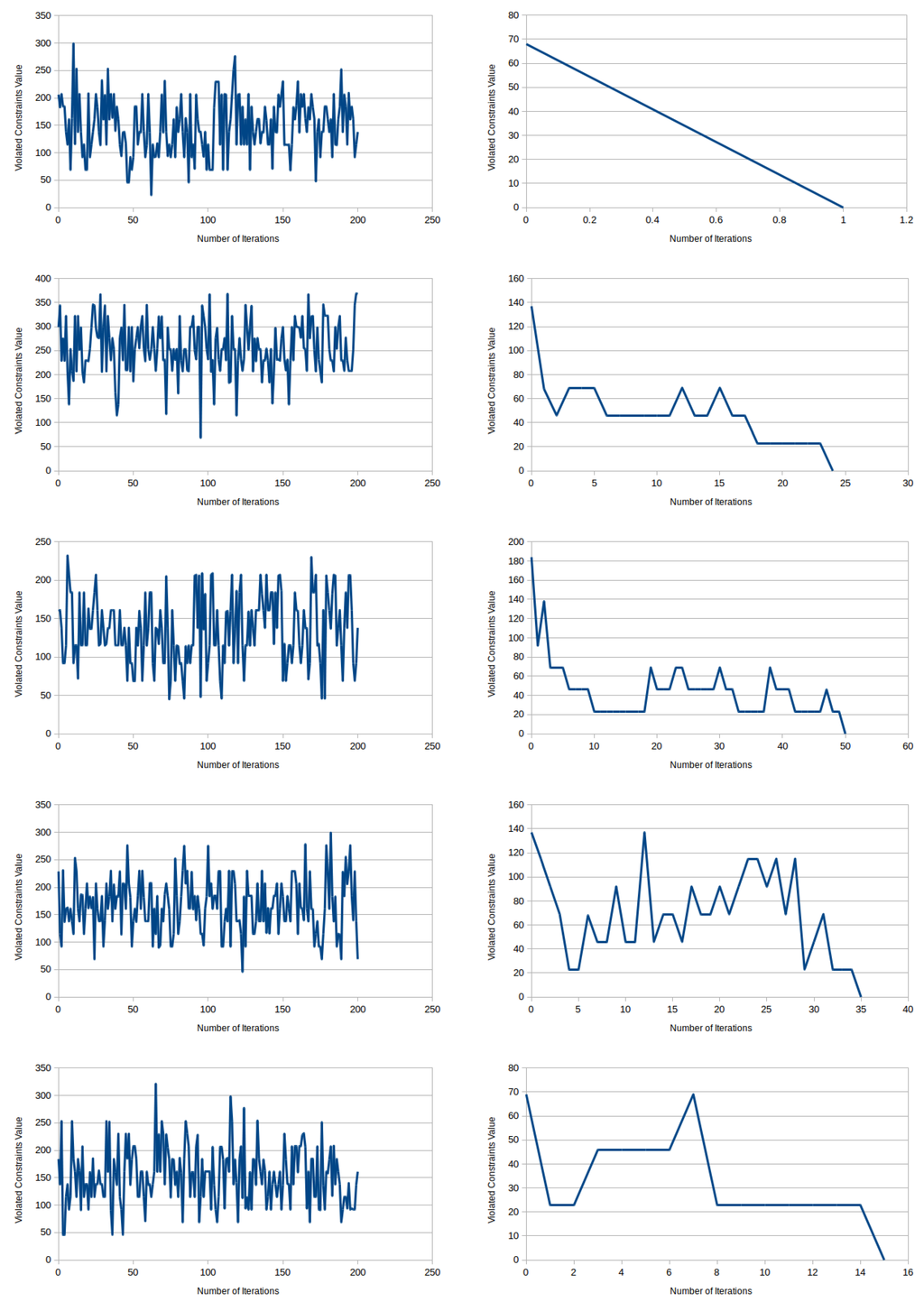
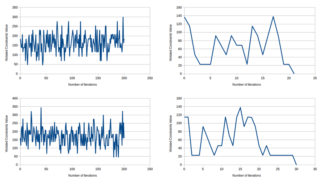
Figure 9.
Comparison of unsatisfied constraints between randomly-parametrized ERE and genetically-optimized ERE.
In Table 5, we compare the percentage of satisfied constraints between a genetically-optimized ERE system with the one whose parameters are assigned values randomly. A genetically-optimized system always tends to achieve a complete solution, where all of the constraints in the SensorDCSP network instance are satisfied and all the entities are at zero positions.
Table 5.
Parameters and the efficiency of optimal solutions obtained from the randomly-parametrized ERE system and genetically-optimized ERE system.
| Randomly-Parametrized ERE System | Genetically-Optimized ERE System | |||||
|---|---|---|---|---|---|---|
| Serial No. | Probability of random- moves | Number of better- moves | Maximum percentage of satisfied constraints | Probability of random- moves | Number of better- moves | Maximum percentage of satisfied constraints |
| 1 | 0.15496815 | 4 | 95.23 | 0.01211132 | 2 | 100 |
| 2 | 0.42432100 | 1 | 86.36 | 0.01194915 | 1 | 100 |
| 3 | 0.10984850 | 2 | 91.49 | 0.01227836 | 2 | 100 |
| 4 | 0.16187531 | 4 | 95.65 | 0.03812959 | 1 | 100 |
| 5 | 0.17335061 | 3 | 89.47 | 0.01582020 | 3 | 100 |
| 6 | 0.18202485 | 4 | 90.90 | 0.06199995 | 2 | 100 |
| 7 | 0.0441960 | 5 | 90.00 | 0.04419600 | 5 | 100 |
4.4. Average Fitness of the ERE System from each Successive Generation of the Genetic Algorithm
Figure 10 demonstrates the variationin the mean and best fitness values of the objective function, i.e., the execution time of the ERE algorithmas the execution of GA proceeds. These values clearly show a steep decrease in the value of the mean of the objective function. Thereafter, a stumbling change occurs in the number of generations. However, the change is considerably less and is confined well within the range. Moreover, pertaining to the best fitness value of the objective function, we observed a quick vanishing after the initial variations, thereby indicating a trivial amount of improvement for longer generations. Further, It is evident that beyond 100 generations, the objective function attains a sufficiently stagnant fitness value and stabilizes.
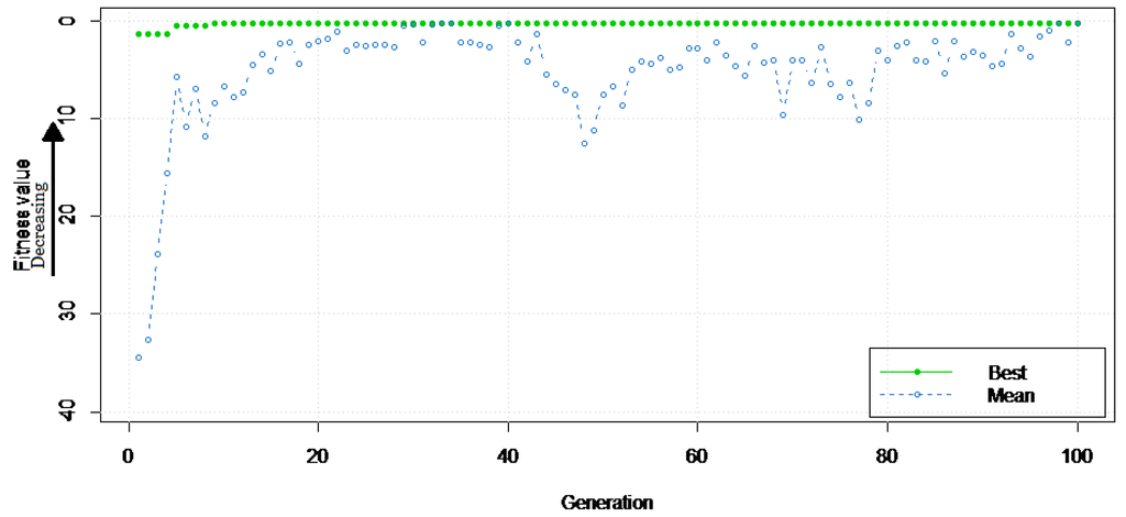
Figure 10.
Fitness value (time to run ERE) vs. generations for the genetic algorithm.
4.5. Variation in Execution Time Corresponding to the Probability of Random-Moves
We examine the execution time of the ERE system to compute a solution with iterative increment over the probability of a random move for a specified number of better-moves before a least move (Figure 11). It can be clearly observed that for the random move with a probabilityless than 0.7, the time for execution is comparably low. This observation further endorses the results derived in Section 4.2 by applying GA. In addition, a steep rise in execution time is noticed when the probability of a random move reaches 12 percent of the value corresponding to each value of the better move before a least move. The results derived here affirm the belief that a high probability of randomness disrupts any solutionstate, and it is of utmost necessity to control the amount of exploration in such systems. Additionally, it is not possible to infer the number of better-moves required before a least move that result in a time-efficientERE solver for the SensorDSCP problem at hand.
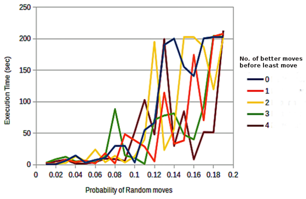
Figure 11.
Variation in execution time vs. probability of a random move for a distinct number of better-moves before a least move.
5. Conclusions
We choose SensorDSCPas a representative of distributed constraint satisfaction problems, and our work primarily focuses on the effective transition of an autonomous system from the current emergent behavior to the desired emergent behavior. We accomplish this by applying GA, though other techniques can also be employed to tweak the parameters of the autonomous entities. The genetic algorithm (GA) is utilized to adjust the simulation parameters in the implementation of the ERE algorithm. Additionally, we studied how the emergent behavior in a non-linear self-organized system is an essential property of local interactions between entities, which have a strong correlation with the system’s parameters. Future work includes the exploration of the impact of previous moves to shape and reason about future outcomes. Adhering to the rule of thumb of autonomous system design, that system parameters are self-adapted to the performance feedback of the system, a more sophisticated algorithm may be explored to auto-adjust the simulation parameters for the specified application domain.
Acknowledgments
The corresponding author would like to take this opportunity to acknowledge Xiaolong Jin, Associate, ICT, Chinese Academy of Sciences, for providing deeper insights from his book “Autonomy Oriented Computing”, which is extensively referred to in this study. The author would also like to acknowledge D.M. Gordon, Department of Biology, Stanford University, for her valued support in providing an understanding of evolutionary processes in complex systems.
Author Contributions
All authors contributed equally to the paper. All authors have read the final manuscript and approved it.
A. Appendix
A.1. Model Functioning Guidelines
Entities and State Variables
The description of the entities and variables of the model developed in this study is provided in Table 6.
Table 6.
Entities and variables in the model developed.
| Entities | Variables/Characteristics | Description |
|---|---|---|
| Mobile Nodes | p-x | x coordinate of the mobile node. |
| p-y | y coordinate of the mobile node. | |
| sensors-in-range | All sensors within its specified range. | |
| tracking-nodes-count | Current node numbers of the sensor nodes tracking it. | |
| Sensor Nodes | p-x | x coordinate of the sensor node. |
| p-y | y coordinate of the sensor node. | |
| mobiles-in-range | All mobiles within its specified range. | |
| Network | num-sensors | Number of sensor nodes in the simulated wireless network. |
| num-mobiles | Number of mobile nodes in the simulated wireless network. | |
| transmission-range | The transmission for the communication of nodes in the network. | |
| k-communicating-sensors | Number of sensor nodes required to track a mobile node within its range. | |
| ERE Algorithm | probability-random | The probability of a random move. |
| number-of-better-moves | The number of better-moves before a least move. | |
| overall-constraints | The number unsatisfied at the present state of the algorithm running. |
Initialization
The user determines the number of mobile and sensor nodes of the network to be created along with the transmission range of the network. The locations of the sensors and the mobile node are randomly initialized at the start using a pseudo-random generator. The ERE algorithm is initialized using the procedure “initialize”, which simulates the autonomous system in accordance with its redefined parameters. Then, the ERE algorithm is executed by the procedure “step” to solve the DSCP. The algorithm parameters either may be determined by the user or through the use of the genetic algorithm using R.
Sub-Models
The sub-model “network” is used to generate a view of the initialized wireless sensor tracking system depicting the sensor and mobile nodes with their locations in the coordinate system.
The sub-model “random-move”, ”least-move” and “better-move” simulate the primitive behaviors random move, least move and better move, respectively, followed by the ERE algorithm entities. The sub-model “f2bl” calls the procedure “better-move” and “least-move” in accordance with the value of the variable number-of-better-moves.
The sub-model “calculate-overall” computes the overall unsatisfied constraints at the present state of the ERE run. The sub-models “evaluate-k-constraints” and “evaluate-range-constraints” evaluate the presently unassigned mobile nodes with exactly k sensors and the number of assignments between sensor nodes to mobile nodes that do not satisfy the range constraint, respectively. The sub-model “environment-evaluation” computes the violation value of an entity with respect to its current position.
Process Overview and Scheduling
When the model starts, the wireless sensor tracking system is created with the characteristics mentioned in the section on entities and state variables. The autonomous system using ERE algorithm is initialized with its inherent parameters using the sub-model “initialize”. Hereby, the sensor and mobiles are placed in the environment along rows and columns. The following steps are executed, in this order, once per time step:
With the execution of the “step” sub-model, at each time step, all sensors decide their respective movements, that is which mobile node they wish to track. This is accomplished in accordance with the three primitive behaviors, namely least move, better move and random move, mentioned before. The chance of each being followed by a sensor depends on the variables, probability-random and number-of-better-moves.
- As the sub-model executes, the sensor nodes consequently determine the mobile node to track with the system, checking whether or not all sensors are at zero positions after all sensors are allowed to move.
- The execution will terminate when a solution with no unsatisfied constraints is obtained. Otherwise, the sub-model will continue to dispatch sensors to move, updating the intermediate solution thus found.
- The plot for the variation of unsatisfied constraints presently is updated after each time step, while the execution of “step” is underway.
How to Use This Model
- Press “setup” to create the wireless sensor tracking system, thereby assigning each sensor and mobile node a randomly-generated position in accordance with the given network parameters.
- Press “initialize” to simulate the ERE environment, with sensor and mobile nodes placed along the rows, while mobiles are along the columns in the autonomous system.
- Press “step” to the start the ERE algorithm to solve the given distributed CSP for the wireless network.
- Press “network” to view the wireless tracking system with the sensor and mobile nodes at their specified positions.
- The num-sensors slider specifies the number of sensor nodes in the wireless sensor tracking system.
- The num-mobiles slider decides how many mobiles nodes will be present in the simulated network.
- The transmission-range slider is used to specify the transmission range for the communication of nodes in the network.
- The k-communicating-sensors slider represents exactly the number of sensor nodes each mobile must be tracked by within its range.
- The probability-random specifies the probability of random move in the ERE algorithm. It may be determined by the user or by using the genetic algorithm with the help of R.
- The number-of-better-moves denotes the number of better moves performed by an entity before a least move. This can be also computed optimally for the given network by using the genetic algorithm.
Conflicts of Interest
The authors declare no conflict of interests.
References
- Ferber, J. Multi-Agent Systems: An Introduction to Distributed Artificial Intelligence; Addison-Wesley Reading: Boston, MA, USA, 1999; Volume 1. [Google Scholar]
- Yokoo, M. Asynchronous weak-commitment search for solving distributed constraint satisfaction problems. In Principles and Practice of Constraint Programming: CP’95; Springer: Berlin, Germany, 1995; pp. 88–102. [Google Scholar]
- Yokoo, M.; Durfee, E.H.; Ishida, T.; Kuwabara, K. The distributed constraint satisfaction problem: Formalization and algorithms. IEEE Trans. Knowl. Data Eng. 1998, 10, 673–685. [Google Scholar] [CrossRef]
- Yokoo, M.; Hirayama, K. Algorithms for distributed constraint satisfaction: A review. Auton. Agents Multi-Agent Syst. 2000, 3, 185–207. [Google Scholar] [CrossRef]
- Silaghi, M.C.; Sam-Haroud, D.; Faltings, B. ABT with asynchronous reordering. In Proc. Of Intelligent Agent Technology (IAT); World Scientific Publishing: Singapore, 2001; pp. 54–63. [Google Scholar]
- Silaghi, M.C.; Sam-Haroud, D.; FALTINGS, B. Asynchronous consistency maintenance. In Proceedings of the International Conference on Intelligent Agent Technology, Maebashi TERRSA, Maebashi City, Japan, 23–26 October 2001; pp. 98–102.
- Silaghi, M.C.; Sam-haroud, D.; Faltings, B. Secure asynchronous search. In Proceedings of the International Conference on Intelligent Agent Technology (IAT’01), Maebashi TERRSA, Maebashi City, Japan, 23–26 October 2001; pp. 400–404.
- Ruttkay, Z. Constraint satisfaction-a survey. CWI Q. 1998, 11, 163–214. [Google Scholar]
- Yokoo, M.; Ishida, T.; Durfee, E.H.; Kuwabara, K. Distributed constraint satisfaction for formalizing distributed problem solving. In Proceedings of the IEEE 12th International Conference on Distributed Computing Systems, Yokohama, Japan, 9–12 June 1992; pp. 614–621.
- Liu, J.; Jin, X.; Tsui, K.C. Autonomy Oriented Computing: From Problem Solving to Complex Systems Modeling; Springer: New York, NY, USA, 2005. [Google Scholar]
- Fernàndez, C.; Béjar, R.; Krishnamachari, B.; Gomes, C. Communication and computation in distributed CSP algorithms. In Principles and Practice of Constraint Programming-CP 2002; Springer: Berlin, Germany, 2002; pp. 664–679. [Google Scholar]
- Zhao, C.; Zhong, N.; Hao, Y. AOC-by-Self-discovery Modeling and Simulation for HIV. In Life System Modeling and Simulation; Springer: Berlin, Germany, 2007; pp. 462–469. [Google Scholar]
- Sycara, K.; Roth, S.F.; Sadeh, N.; Fox, M.S. Distributed constrained heuristic search. IEEE Trans. Syst. Man Cybern. 1991, 21, 1446–1461. [Google Scholar] [CrossRef]
- Mason, C.L.; Johnson, R.R. DATMS: A framework for distributed assumption based reasoning. In Distributed Artificial Intelligence; Morgan Kaufmann Publishers Inc.: Burlington, MA, USA, 1989; Volume 2, pp. 293–317. [Google Scholar]
- Doyle, J. A truth maintenance system. Artif. Intell. 1979, 12, 231–272. [Google Scholar] [CrossRef]
- Huhns, M.N.; Bridgeland, D.M. Multiagent truth maintenance. IEEE Trans. Syst. Man Cybern. 1991, 21, 1437–1445. [Google Scholar] [CrossRef]
- Conry, S.E.; Kuwabara, K.; Lesser, V.R.; Meyer, R.A. Multistage negotiation for distributed constraint satisfaction. IEEE Trans. Syst. Man Cybern. 1991, 21, 1462–1477. [Google Scholar] [CrossRef]
- Bond, A.H.; Gasser, L. An analysis of problems and research in DAI. In Readings in DAI; Morgan Kaufmann Publishers: San Francisco, CA, USA, 1988. [Google Scholar]
- Russell, S.; Norvig, P.; Intelligence, A. A modern approach. In Artificial Intelligence; Prentice-Hall: Egnlewood Cliffs, NJ, USA, 1995; Volume 25. [Google Scholar]
- Mackworth, A.K.; Freuder, E.C. The complexity of some polynomial network consistency algorithms for constraint satisfaction problems. Artif. Intell. 1985, 25, 65–74. [Google Scholar] [CrossRef]
- Kirkpatrick, D.G.; Hell, P. On the complexity of general graph factor problems. SIAM J. Comput. 1983, 12, 601–609. [Google Scholar] [CrossRef]
- Bejar, R.; Krishnamachari, B.; Gomes, C.; Selman, B. Distributed constraint satisfaction in a wireless sensor tracking system. In Proceedings of the Workshop on Distributed Constraint Reasoning, International Joint Conference on Artificial Intelligence, Seattle, WA, USA, 4 August 2001.
- Gutowitz, H. Cellular Automata: Theory and Experiment; MIT Press: Cambridge, MA, USA, 1991; Volume 45. [Google Scholar]
- Liu, J.; Tang, Y.Y.; Cao, Y. An evolutionary autonomous agents approach to image feature extraction. IEEE Trans. Evolut. Comput. 1997, 1, 141–158. [Google Scholar] [CrossRef]
- Gu, J. Efficient local search for very large-scale satisfiability problems. ACM SIGART Bull. 1992, 3, 8–12. [Google Scholar] [CrossRef]
- Gordon, D.M. 10 What We Don’t Know about the Evolution of Cooperation. In Cooperation and Its Evolution; MIT Press: Cambridge, MA, USA, 2013; p. 195. [Google Scholar]
- Belew, R.K.; McInerney, J.; Schraudolph, N.N. Evolving networks: Using the genetic algorithm with connectionist learning. In Citeseer; Addison-Wesley: Boston, MA, USA, 1990; pp. 511–547. [Google Scholar]
- Tisue, S.; Wilensky, U. Netlogo: A simple environment for modeling complexity. In Proceedings of the International Conference on Complex Systems, Boston, MA, USA, 16–21 May 2004; pp. 16–21.
- Matsumoto, M.; Nishimura, T. Mersenne twister: A 623-dimensionally equidistributed uniform pseudo-random number generator. ACM Trans. Model. Comput. Simul. (TOMACS) 1998, 8, 3–30. [Google Scholar] [CrossRef]
- Scrucca, L. GA: A package for genetic algorithms in R. J. Stat. Softw. 2012, 53, 1–37. [Google Scholar]
- Statistical Package, R. R: A language and environment for statistical computing. R Foundation for Statistical Computing: Vienna, Austria, 2009. [Google Scholar]
© 2015 by the authors; licensee MDPI, Basel, Switzerland. This article is an open access article distributed under the terms and conditions of the Creative Commons Attribution license (http://creativecommons.org/licenses/by/4.0/).