Scalable Univariate and Multivariate Time-Series Classifiers with Deep Learning Methods Exploiting Symbolic Representations

Abstract

Time-series classification (TSC) is an important task across sciences. Symbolic representations (especially SFA) are very effective at combating noise. In this paper, we employ symbolic representations to create state-of-the-art time-series classifiers, with the aim to advance scalability without sacrificing accuracy. First, we create a graph representation of the time series based on SFA words. We use this representation together with graph kernels and an SVM classifier to create a scalable time-series classifier. Next, we use the graph representation together with a Graph Convolutional Neural Network to test how it fares against state-of-the-art time-series classifiers. Additionally, we devised deep neural networks exploiting the SFA representation, inspired by the text classification domain, to study how they fare against state-of-the-art classifiers. The proposed deep learning classifiers have been adapted and evaluated for the multivariate time-series case and also against state-of-the-art time-series classification algorithms based on symbolic representations.

1. Introduction

Time-series classification (TSC) is an important task across many branches of science. Indicative applications of TSC are seizure detection [1], earthquake monitoring [2], insect classification [3], applications in power systems [4], and other applications [5,6,7,8,9,10,11,12,13]. Symbolic representations (especially SFA) [14] have been proven to be very effective in combating noise. To this end, this paper aims to incorporate symbolic representations to create state-of-the-art time-series classification algorithms, aiming to advance their scalability without sacrificing accuracy. More specifically, this paper aims to answer the following research questions (RQs):

• RQ1. How would a classifier built on top of graph representations of SFA words perform in terms of accuracy and execution time? Our first attempt to answer this question is through the use of graph kernels, which are more scalable than Graph Neural Networks, with an SVM classifier on top.
• RQ2. Closely linked with RQ1, we take the graph representation with SFA words and combine it with Graph Convolutional Neural Networks to see how the resulting classifier would fare against the state of the art.
• RQ3. For this research question, we aim to answer whether SFA, together with state-of-the-art deep learning methods adapted from the text classification domain, can also provide state-of-the-art accuracy and execution times for multivariate time-series classification.
• RQ4. Finally, we aim to answer whether SCALE-BOSS-MR [15], a state-of-the-art symbolic time-series classifier, can be adapted to the multivariate use case and whether it provides state-of-the-art accuracy and execution time.

To answer the above research questions, this paper makes the following contributions:

1.

We use a graph representation together with a symbolic representation to represent time-series as a graph. First, we use this representation together with graph kernels and an SVM classifier to create SCALE-BOSS-GRAPH.

2.

We use the graph representation of time-series in conjunction with a Graph Convolutional Neural Network to see whether it can attain state-of-the-art accuracy and execution time.

3.

We adapt state-of-the-art neural network architectures from the text classification domain, and we use them in conjunction with symbolic representation to create state-of-the-art deep learning symbolic time-series classifiers. We also adapt the proposed deep learning methods to the multivariate use case and compare them against state-of-the-art deep learning methods.

4.

We adapt SCALE-BOSS-MR to the multivariate use case, and we compared the adapted version SCALE-BOSS-MR-MV to state-of-the-art time-series classifiers.

2. Related Work

2.1. Methods Using Symbolic Representations

Symbolic representations have been used widely in the time-series literature for dimensionality reduction, smoothing, and combating noise. Most of the recent TSC literature has used SFA [14] or SFA in conjunction with SAX [16]. SFA is a state-of-the-art symbolic representation that uses Fourier coefficients to represent the time-series. SFA has been proven to be very efficient in combating noise.

In [17], the authors present SAX-VSM. SAX-VSM uses SAX as its symbolic representation. SAX-VSM pairs SAX representations with Term Frequency–Inverse Document Frequency (TF-IDF) weighting. After the training set is transformed into SAX words, a tf-idf vector is created for each class as a whole. In the next step, the set of targets time-series is transformed into SAX words, and the Term-Frequency (TF) vector is created for each time-series in the target set. To classify a time-series, the cosine similarity between the TF vectors of that series and of the classes’ centers is computed.

BOSS [18] is the first time-series classification algorithm to use SFA. However, the high computational load of BOSS made it impractical for many applications. To this end, in [19], the authors present BOSS-VS, a time-series classification algorithm that uses SFA but is geared towards scalability.

In [20], the authors present WEASEL, a middle ground between BOSS and BOSS-VS in terms of computational complexity and accuracy. WEASEL uses multiple window sizes and bigrams with a chi-squared feature extraction pipeline and a linear classifier on top.

In [21], the authors present K-BOSS-VS, a time-series classifier that is a middle ground between BOSS and BOSS-VS in terms of computational complexity and accuracy. The main idea of K-BOSS-VS is that, instead of having a single representative for each class as in BOSS-VS, the K-means clustering algorithm is applied to pick K representatives for each class.

In [22,23], the authors present MRSQM, a framework that uses multiple symbolic representations for scalable and accurate TSC. MRSQM uses both SFA and SAX representations and efficient sequence mining to extract important time-series features.

In [24], the authors present BOSS-SCALE, which generalizes the process of K-BOSS-VS to use a pluggable classifier on top of the SFA Term-Frequency vectors.

In [25], the authors present WEASEL 2.0, an updated version of WEASEL that incorporates first-order differences and dilation together with randomization to provide a state-of-the-art scalable classification algorithm.

In [15], the authors extend SCALE-BOSS into SCALE-BOSS-MR. SCALE-BOSS-MR uses multiple window sizes, first-order differences, and dilation. On top of these representations, SCALE-BOSS-MR uses a pluggable classifier like SCALE-BOSS. Instead of using randomization to achieve scalability, SCALE-BOSS-MR uses carefully crafted optimization parameters that aim to balance between accuracy and scalability.

SCALE-BOSS-MR proved to be significantly faster than both MRSQM and WEASEL 2.0 with minimal loss in accuracy.

In summary, SAX-VSM and BOSS-VS are aimed towards scalability. BOSS aims only at high accuracy and it is not scalable. WEASEL is proposed as a middle ground between BOSS and BOSS-VS, achieving high accuracy and relative scalability. SCALE-BOSS achieves great accuracy with execution time only marginally worse than BOSS-VS. WEASEL 2.0 provides very high accuracy with execution time better than WEASEL thanks to randomization. Finally, SCALE-BOSS-MR achieves state-of-the-art accuracy while retaining state-of-the-art execution time.

There are not many works proposing symbolic classifiers for multivariate time-series. In [26] the authors present WEASEL+MUSE, which extends WEASEL to the multivariate use case while incorporating first-order differences.

2.2. Methods Using Convolutional Kernels

In [27] the authors present ROCKET, a scalable and highly accurate TSC classifier. ROCKET uses a large number (10000) of Convolutional kernels paired with a linear classifier.

In [28] the authors present a significantly faster version of ROCKET that retains state-of-the-art accuracy called MiniRocket. It manages to do so by using a significantly lower number of Convolutional kernels.

2.3. Methods Using Deep Learning

In [29] the authors present the MLP, FCN and ResNet architectures. The MLP architecture uses three fully connected layers, each with 500 neurons. The architecture uses dropout [30] to prevent overfitting and the ReLU activation function [31] to prevent saturation of the gradient. Regarding FCN, the basic blocks of the architecture are a convolutional layer followed by Batch Normalization [32]. The architecture stacks three such blocks, followed by a global average pooling layer and a softmax layer. The authors adapt the ResNet architecture [33] for time-series classification. The proposed architecture uses three residual blocks with filters of size $k=\{64,128,128\}$. The three residual blocks are stacked and followed by a global average pooling layer and a softmax layer.

In [34] the authors present a Graph Convolutional Neural Network (GCN) for graph classification. Their architecture stacks two Graph Convolution layers followed by a Mean Pooling operation, two fully connected layers, and finally a SoftMax layer.

In [35] the authors present CNNClassifier. The architecture comprises two 1-D convolutional layers followed by a fully connected layer.

The authors in [36] aim to build a model that is conceptually straightforward and computationally lightweight. They propose the EncoderClassifier. The model consists of convolutional layers, an attention layer to summarize the time axis, and finally a fully connected layer to obtain the desired dimensionality. The convolutional network consists of three convolutional blocks with two factor max pooling layers between them. Each convolutional block comprises 1-D convolutions followed by instance normalization, PRelu, and a dropout layer. After the convolutional layer the results are passed to an attention layer. The results of the attention layer are passed through a fully connected layer and an instance normalization layer.

The InceptionTime classifier proposed in [37] is an ensemble of deep Convolutional Neural Network (CNN) models, inspired by the Inception-v4 architecture. InceptionTime proposes the use of BottleNeck and Multiplex Convolutions. The BottleNeck operation consists of 1-D Convolutions with unit kernel size. The main idea of multiplex Convolutions is to learn in parallel different Convolution layers of different kernel sizes. The composition of an Inception network classifier contains two different residual blocks, compared to ResNet, which comprises three. For the Inception network, each block is composed of three Inception modules rather than traditional fully convolutional layers. Each residual block’s input is transferred via a shortcut linear connection to be added to the next block’s input, thus mitigating the vanishing gradient problem by allowing a direct flow of the gradient.

In [38] the authors create hand-crafted filters in order to detect certain patterns in time-series. Those filters are fixed and do not change during training. The authors modify existing architectures (FCN and Inception time) and through their evaluation show that incorporating the fixed filters improves accuracy. More specifically, the authors propose three types of filters: (a) increasing trend, (b) decreasing trend, and (c) peak detection.

In [39] the authors present the LITE classifier. LITE uses 9814 training parameters while achieving state-of-the-art performance. LITE uses DepthWiseSeperableConvolutions, which are boosted by three techniques:(a) multiplexing convolutions [37,40], (b) dilated convolutions [41], and (c) custom filters [38].

2.4. Multivariate Time Series Classification

In [42] the authors present two methods of Multivariate Time Series classification (MTS) representation using SAX. In the first one, multivariate words are generated by combining the symbols of each attribute at a particular time, and a bag-of-patterns approach is used to classify MTS. This way, the method considers the correlation between the time-series by combining individual representations of attributes. However, this approach significantly increases the size of the individual word for a large number of attributes. This potentially limits the effectiveness in terms of accuracy of the method since longer words could potentially carry less information because of the curse of dimensionality. The authors also propose a stacked bag-of-patterns approach. This approach concatenates the representations of multiple univariate time-series into one by stacking the term frequency vectors for each attribute column-wise.

In [43] the authors propose a method that uses a symbolic representation to perform multivariate time-series (MTS) classification. The authors propose a new symbolic representation for MTS denoted as SMTS. SMTS considers all attributes of MTS simultaneously, rather than separately, to extract information contained in relationships. An elementary representation is used that consists of the time index and the values (as well as first-order differences) of the individual time-series as columns. Each MTS is concatenated vertically and each instance is labeled with the class of the corresponding time-series. A tree learner is applied to the simple representation and each instance is assigned to a terminal node of the tree. This means that a symbol is associated for each time index (instance), instead of intervals of the time-series. With R terminal nodes, the dictionary contains R symbols. After each instance has been associated with a symbol from each tree of the ensemble, the term frequency vector for each symbol is computed and the term frequency vectors are stacked column-wise as in the Stacked-Bag-of-Patterns in [42].

In [26] the authors extend WEASEL to work with multivariate datasets. The authors use the WEASEL pipeline for each feature separately and then they create the final term frequency vector by stacking the separate term frequency vectors column-wise. The WEASEL-MUSE also uses first-order differences to enhance accuracy.

In order to adapt ROCKET [27] to multivariate datasets, kernels are randomly assigned dimensions and then weights are generated for each channel. This way, ROCKET retains scalability in the multivariate use case.

The interested reader can read a detailed survey of multivariate time-series classification in [44].

3. Graph Kernel Preliminaries

The idea behind graph kernels is to create a kernel matrix that can be used with off-the-shelf machine learning models to make predictions. The kernel matrix measures the similarity between all pairs of graphs. In order for the kernel matrix to be valid, the matrix has to be symmetric with positive eigenvalues.

The key idea of kernel methods is to design a feature representation of a given graph as a bag-of-words. In this case, we need a feature representation $\varphi$(.) such that $K(G1,G2)={\left(\varphi \left(G1\right)\right)}^{⊺}·\varphi \left(G2\right)$, where K is the kernel matrix, $G1$ is the first graph and $G2$ is the second graph. The naive representation is to use words as nodes. The problem with this approach is that we can have the same representation for very different graphs. This happens because this approach does not consider connectivity between the nodes of each graph.

To address this issue, we are using the Weisfeiler–Lehman (WL) graph kernel. The main idea of the WL graph kernel [45] is to have an efficient feature descriptor $f\left(G\right)$ by exploiting the neighborhood structure of the graph to iteratively enrich the node vocabulary, i.e., the set of possible labels for the graph nodes. The WL is a generalized version of node degrees because node degrees provide 1-hop information, whereas WL generalizes this to the k-hop. The algorithm to achieve this is called WL isomorphism test or color refinement.

Color Refinement

This section describes the color refinement procedure behind the WL kernel.

Given a graph G with nodes V, the process assigns an initial color $c^{\left(0\right)}\left(v\right)$ to each node v. Then, it iteratively refines colors as follows: $c^{(k+1)}\left(v\right)=HASH(c^{\left(k\right)}\left(v\right),c^{\left(k\right)}\left(u\right))$, with $u\in neib\left(v\right)$, and $HASH$ maps different inputs (node labels) to different colors. After k steps of color refinement, it summarizes the structure of the K-Hop neighborhood.

Figure 1, Figure 2, Figure 3 and Figure 4 provide an example of the application of the WL graph kernel for two graphs.

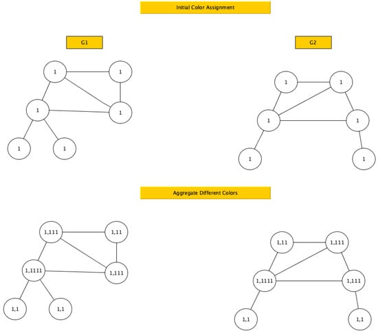
Figure 1. Iteration 0 of color refinement.

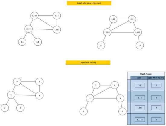
Figure 2. Hashing after the first iteration of color refinement.

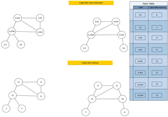
Figure 3. Hashing after the second iteration of color refinement.

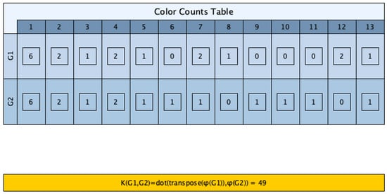
Figure 4. Vector representation of the two graphs.

Initially, all nodes of the two graphs get a color (label) of 1. Next, for each node it computes the next label. The next label for each node is created by merging the colors of its neighbors together with its previous color. For example, the top left node of $G1$ gets a label of (1,111), whereas the top left node of $G2$ gets a label of (1,11).

After it has created the new color for each node, the processes pass it through the hash function. For example, according to the hash table, (1,111) gets a new color 4, while (1,11) gets a new color 3.

Figure 3 shows the second iteration of the color refinement procedure.

Figure 4 provides the feature representation of the two graphs, by counting the total number of color occurrences in each graph.

4. Deep Learning Preliminaries

4.1. Convolutional Neural Networks

The original purpose of Convolutional Neural Networks (CNNs) [46,47] is to detect certain features in an image. The early layers of a CNN detect local visual features, and later layers of a CNN take those features and combine them to produce higher-level features.

In order for a CNN layer to detect features, the main idea is to pass a filter across the image (or more generally, a tensor) with a process called convolution.

The convolution operation retains spatial information and essentially performs a point-wise multiplication of the patch of an image with the filter followed by an addition of the point-wise multiplication results to extract the final value.

Usually, convolutional layers are followed by a pooling operation for dimensionality reduction. Pooling is an operation of applying a small filter that returns either the maximum value (max pooling) or the average (average pooling) in the specific window of the tensor.

4.2. Recurrent Neural Networks

RNNs [48,49,50] are created to handle sequence information. The RNN has a single hidden layer, but it also has a memory buffer that stores the output of the hidden layer and feeds it back into the layer along with the next element from the input sequence. This means that the RNN processes each input of the sequence together with context information from the previous inputs. One problem with RNNs is that, while they can process a sequence of inputs, they have the problem of vanishing gradients. This is because training an RNN to process a sequence of inputs requires the error to be backpropagated through the entire length of the RNN.

4.3. Long Short Term Memory

In [51] the authors present the Long Short Term Memory (LSTM) cells that aim to solve the vanishing gradient problem.

In LSTMs, the propagation of the activations within the cell through time is controlled by three components called gates: the forget gate, the input gate, and the output gate. The forget gate determines which activations in the cell should be forgotten at each time step; the input gate decides how the activations in the cell should be updated in response to the new input. Finally, the output gate controls what activations should be used to generate the output in response to the current input.

The forget gate takes the concatenation of the input and the hidden state and passes this vector through a layer of neurons that uses a sigmoid activation function. The output of this forget layer is a vector of values in the range 0 to 1. The cell state is then multiplied by this forget vector. The result of this multiplication is that activations in the cell state that are multiplied by components in the forget vector with values near 0 are forgotten, and activations that are multiplied by components with values near to 1 are remembered. Next, the input gate decides what information should be added to the cell state.

The procedure works as follows. The gate decides which elements in the cell state should be updated and what information should be included in the update. The concatenated input $x_t$ plus hidden state $h_{t-1}$ is passed through a layer of sigmoid units to generate a vector of elements, the same width as the cell, where each element in the vector is in the range 0 (no update) to 1 (to be updated). At the same time that the filter vector is generated, the concatenated input and hidden state are also passed through a layer of $tanh$ units. The final stage of processing in an LSTM is to decide which elements of the cell should be output in response to the current input.

A candidate output vector is generated by passing the cell through a $tanh$ layer. At the same time, the concatenated input and propagated hidden state vector are passed through a layer of sigmoid units to create another filter vector. The actual output vector is then calculated by multiplying the candidate output vector by this filter vector. An RNN with LSTM cells is called an LSTM network.

4.4. Attention

In [52] the authors present the attention mechanism to address the bottleneck problem that arises with the use of a fixed-length encoding vector, where the decoder would have limited access to the information provided by the input. This is thought to become especially problematic for long sequences.

The main idea of the attention mechanism is to have a context vector per time step. The intuition behind the context vector is that now the context vector attends to the relevant part of the input sequence.

The attention mechanism is composed of three parts:

1.

Alignment scores: The alignment scores e indicate how well the elements of the input sequence align with the current output. The alignment scores are computed by $e=tanh\left(dot\right(x,W)+b)$, where W is the weight matrix of the attention layer, b is the bias of the attention layer and x is the input of the attention layer.

2.

Weights: The weights a are computed by passing a softmax to e. That is, $a=softmax\left(e\right)$

3.

Context Vector: The context vector c is computed by the dot product of x and a. That is, $c=dot(x,a)$

5. Proposed Methods

5.1. SCALE-BOSS-GRAPH

The SCALE-BOSS-GRAPH framework fuses graph and symbolic representations.

The idea of the graph-based symbolic representation comes from the input of BOSS, BOSS-VS and K-BOSS-VS. More specifically, after each time-series is encoded in SFA words, each successive word is connected to the one after it to create a graph. Figure 5 shows examples of graph-based symbolic representations. For example, for the first time-series in the figure, the first word “acbb” is connected with the second word “acbb”, which in turn is connected with the third word “acbc” and so on. Each time-series in the dataset is encoded as a graph and the nodes of the graph are labeled using the SFA representation.

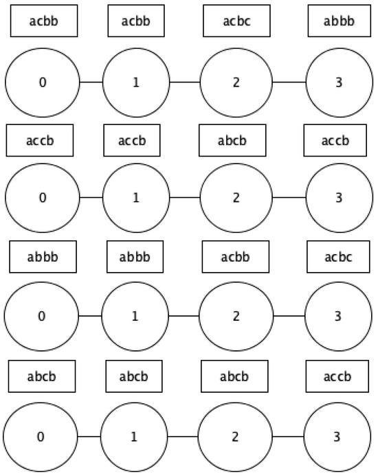
Figure 5. Graph-based symbolic representation.

The workflow of SCALE-BOSS-GRAPH is as follows:

1.

In the first step the training set is converted to its symbolic representation. In our instantiation we have chosen SFA but the choice of the symbolic representation is orthogonal to the framework.

2.

Next, we create the graph-based symbolic representation for the training set.

3.

In the third step, we create the Kernel for the training set. For this instantiation, we have chosen the WL graph kernels [45] with Vertex Histogram kernel [53] as the base kernel. The choice of the kernel is orthogonal to the method. We have chosen WL with Vertex Histogram as a base kernel for scalability reasons. More concretely WL proved to be amongst the fastest graph kernels with very good accuracy results. We experimented with other graph kernels, but most were orders of magnitude slower than WL with no gains in terms of accuracy. In addition to this, as already pointed out, the WL kernel is a generalization of nodes’ degrees since these provide one-hop neighborhood information, whereas WL kernel generalized this to K-hop information.

4.

Then, we convert the test set to its symbolic representation, and the Graph-based symbolic representation.

5.

Then, we create the kernel representation for the test set.

6.

The SVC classifier is trained on the precomputed kernel for the training set.

We also used the graph-based symbolic representation as an input to a CNN [34].

5.2. Proposed Networks for the Univariate Case

In this section we describe the neural network architectures that have been studied to exploit the symbolic representation of univariate time-series. In all of the proposed neural network architectures, the input is constructed as follows:

1.

First, the raw time-series is converted to the SFA representation.

2.

Then each of the resulting SFA words is converted to integers according to the following scheme.

(a)

The most common SFA word is assigned the integer 2.

(b)

The second most common SFA word is assigned the integer 3 and so on for all the next in frequency SFA words.

(c)

The integer 0 is used for padding and the integer 1 is reserved for the Out-of-Vocabulary token.

Figure 6 depicts the architecture of the LSTM-CNN neural network. The first layer is an embedding layer that takes the sequence of integers and creates embeddings. Embedding vectors have a length of 32. Then, the embedding layer is fed into a CNN followed by a MaxPooling layer. The CNN has a filter size 32 and kernel size of 3. After that, the results of the MaxPooling layer are fed into an LSTM layer. The LSTM is followed by a batch normalization layer that aims to help the network train faster and achieve better accuracy. Next, we have a Dropout layer to prevent overfitting. Finally, a fully connected layer does the classification.

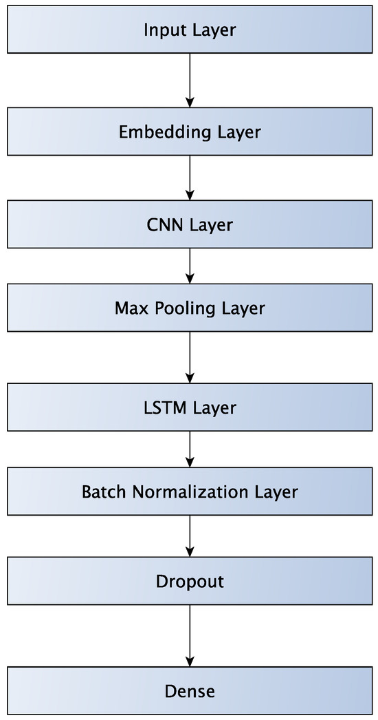
Figure 6. LSTM-CNN network.

Different CNN architectures could be used if we would like to make the proposed architecture deeper. However, keeping the architecture relatively shallow has positive effects on execution time. Also, according to our tests, making the architecture deeper did not necessarily help in terms of accuracy.

In our evaluation section, we compare our proposed architectures with ResNet and it appears to be significantly faster and more accurate.

Figure 7 shows the architecture of a network that combines Bidirectional LSTM with a self-attention layer. A Bidirectional LSTM adds a second LSTM layer that processes the data in reverse (right-to-left). Thus, Bidirectional LSTM provides the model with a complete understanding of the context surrounding a given point in the sequence. The first layer is an embedding layer that takes the sequence of integers and creates embeddings. The embeddings have a vector length of 32. The embeddings are fed into an LSTM layer that is followed by an attention layer, which is followed by a batch normalization layer and a dropout layer. Finally, a Fully Connected layer does the classification.

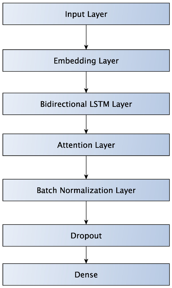
Figure 7. LSTM-Attention network.

Figure 8 shows a neural network architecture that augments the LSTM-Attention network with a CNN layer. The CNN layer is placed before the Bidirectional LSTM layer and is followed by a MaxPooling layer. The CNN has a filter size of 32 and a kernel size of 3. The purpose of the CNN layer is to improve accuracy, but also to significantly reduce execution time. The CNN layer performs dimensionality reduction (via Max Pooling) and thus reduces the complexity of the step after it.

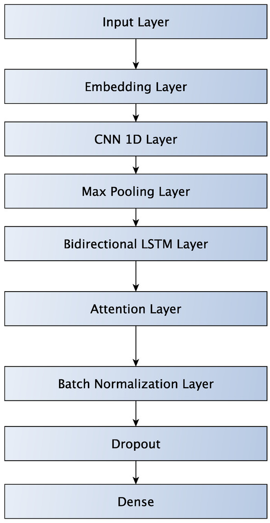
Figure 8. LSTM-Attention-CNN network.

Finally, in Figure 9 we see the LSTM-Attention-CNN2 network that augments the LSTM-Attention-CNN network with an additional CNN layer followed by a MaxPooling layer. The first CNN has a filter size of 32 while the second CNN has a filter size of 16, and both have a kernel size of 3. The extra CNN Layer aims to reduce execution time.

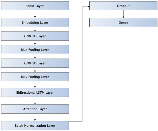
Figure 9. LSTM-Attention-CNN2 network.

The algorithms proposed were implemented on top of pyts [54], GraKeL [55], scikit-learn [56], Keras [57] and StellarGraph [58].

5.3. Merging Strategies for the Multivariate Use Case

In the case of multivariate time-series, there are two strategies to handle the multiple attributes: The BAG and the STACK strategies that are used in both the proposed Deep Learning methods and the proposed extension of SCALE-BOSS-MR (SCALE-BOSS-MR-MV or SBMR-MV). More concretely, suppose we have a time-series with two attributes Attr0 and Attr1. Attr0 contains the sequence “aaaa bbbb” and Attr1 contains the sequence “cccc dddd”. In the BAG case we create the sequence “aaaa bbbb cccc ddd” and then we create the Term-Frequency vector (in the SBMR-MV case) or we pass it into the embedding layer (in the Deep Learning algorithm case.) In the STACK case we create a term frequency vector (or a vectorized representation by an Embedding Layer) for Attr0 and then a term frequency vector (or an Embedding Layer output) for Attr1. Then we concatenate the two vectorized representations horizontally (column-wise) to obtain the final vectorized representation.

5.4. Proposed Multivariate Neural Networks

In the BAG case, each attribute of a multivariate time-series is transformed into its symbolic representation, and the symbolic representations are then fused. Then these are passed on to an embedding layer. In the BAG case, the relationships between attributes are not retained.

From then on the process is the same as for the univariate time-series.

Figure 10 shows the workflow for LSTM-Attention-CNN2 with the BAG workflow.

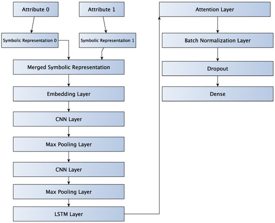
Figure 10. Depiction of the BAG version of LSTM-Attention-CNN2 neural network.

In the STACK case, each attribute is transformed into a symbolic representation, which is fed into an embedding layer. Then, the embeddings are concatenated to form the final embedding of the input sequence.

In Figure 11 we can see the workflow for LSTM-Attention-CNN2 with the STACK workflow.

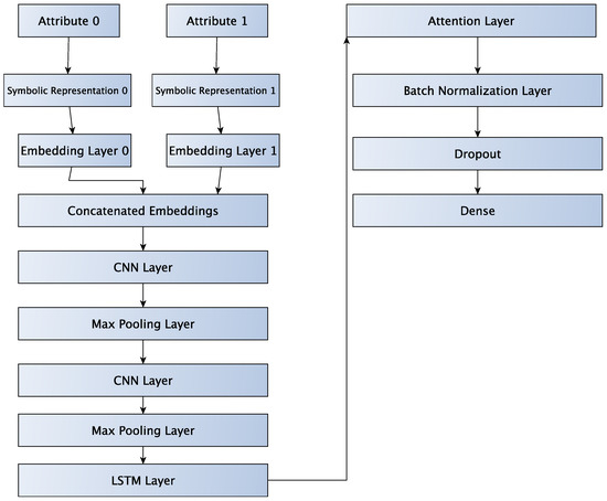
Figure 11. Depiction of the STACK version of LSTM-Attention-CNN2 neural network.

5.5. The SCALE-BOSS-MR-MV (SBMR-MV) Algorithm

Before diving deeper into the specifics of SBMR-MV, we explain in more detail the Merging used in SBMR-MV. More concretely in the BAG case, the vocabularies for all the attributes of the time-series get merged to create a single vocabulary and then a term frequency vector is created. For example, the word aaaa for attribute 0 and the word aaaa for attribute 1 will be in the same bag, which now has a term frequency of 2 for time-series 0. This is because the word aaaa for attribute 0 has a term frequency value of 1 for time-series 0 and the word aaaa for attribute 1 also has a term frequency of 1. When the two get merged to create the final Term-Frequency vector for the BAG strategy, we get a Term-Frequency value of 2. The BAG merging strategy is shown in Figure 12.

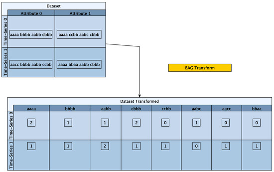
Figure 12. BAG merging strategy example for SBMR-MV.

In the STACK case, each attribute is transformed into its symbolic representation and then a Term Frequency vector is created for each attribute. Then the term frequency vectors are stacked column-wise to produce the final term frequency vector. In contrast to the BAG strategy, when using the STACK merging strategy, the vocabularies for each attribute remain distinct and the term frequency vectors are in effect stacked horizontally (column-wise). For example the word aaaa for attribute 0 is denoted as “aaaa Atr0” and is different than the word aaaa for attribute 1 that is denoted as “aaaa Atr1”. In the STACK merging strategy, both “aaaa Atr0” and “aaaa Atr1” get a Term-Frequency value of 1 for time-series 0.

The STACK merging strategy is shown in Figure 13.

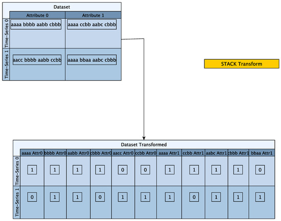
Figure 13. STACK merging strategy example.

The final Term Frequency vector is then passed to the classifier and the procedure from then on is the same as in SCALE-BOSS-MR.

Algorithm 1 describes the SCALE-BOSS-MR-MV (SBMR-MV) process in detail. Lines 1 through 16 describe the inner method of SBMR-MV.

In lines 4 to 7, we apply dilation to each attribute of the input time-series.

Then, in lines 8 through 12, we create the term frequency vector and transform it either using bag or stack merging strategy. Then, in line 13 we merge the current term frequency vector with the global term frequency vector to create the final term frequency vector that will be passed to the classifier. In lines 18 and 19, we create the global term frequency vectors for the train and test sets, respectively. In line 20 we run SBMR-MV-inner. This is a helper function for creating the term frequency vector from the input time-series for the training set. In line 23 we run the SBMR-MV-inner for the first-order differences of the training set. In line 24 we fit the classifier with the term frequency vector of the training set. In line 25 we run SBMR-MV inner for the test set. In line 28 we run the SBMR-MV-inner for the first-order differences of the test set. Finally, in line 29 we get the predicted values for the test set.

The algorithm has two sets of hyperparameters, the window size and the dilation size. The window size allows SBMR-MV to see the input at different granularities similar to WEASEL. Dilation allows the algorithm to see parts of the input that are further ahead.

Algorithm 1: SCALE-BOSS-MR-MV (SBMR-MV) algorithm.

6. Evaluation

6.1. Experimental Setting

We have chosen mean accuracy and mean execution time as the measures of choice.

We define execution time (Total_time) as the total execution time (training time plus test time) of each method for each dataset. Total_Time_Mean is the mean execution time across all datasets. Accuracy_Mean is the mean accuracy across all datasets.

We did that because all of the methods in the literature [15,18,19,20,24,25] use accuracy as a measure of qualitative performance. In addition to that, we used mean execution time as a measure of computational efficiency.

Our tests were performed on a mid 2015 Macbook with a 2.2 Ghz Intel Core i7 and 16 GB of RAM.

Table 1 shows the characteristics of the datasets used for the evaluation of the univariate case. We have chosen the eight datasets from the UCR archive [59] with the largest training set.

Table 1. Characteristics of the datasets.

Name	Train_Size	Test_Size	n_Classes	n_Timestamps
Crop	7200	16,800	24	46
FordB	3636	810	2	500
FordA	3601	1320	2	500
NonInvasiveFetalECGThorax2	1800	1965	42	750
NonInvasiveFetalECGThorax1	1800	1965	42	750
PhalangesOutlinesCorrect	1800	858	2	80
HandOutlines	1000	370	2	2709
TwoPatterns	1000	4000	4	128

In Table 2 we see the characteristics of the multivariate datasets.

Table 2. Description of the multivariate datasets.

Name	Train_Size	Test_Size	NumDimensions	n_Timestamps	n_Classes
ArticularyWordRecognition	275	300	9	144	25
EthanolConcentration	261	263	3	1751	4
FingerMovements	316	100	28	50	2
SelfRegulationSCP1	268	293	6	896	2
UWaveGestureLibrary	120	320	3	315	8

We have chosen five UEA multivariate datasets. We have chosen datasets that have large enough trainSize, contain no null values, and have at least 40 timestamps.

In our evaluation, we measured the following:

1.

The performance, in terms of accuracy and execution time for SCALE-BOSS-GRAPH for the univariate use case.

2.

The performance, in terms of accuracy and execution time of the proposed SFA-enhanced neural network classifiers in the univariate use case.

3.

The performance, in terms of accuracy and execution time of the proposed SFA-enhanced neural network classifiers in the multivariate use case.

4.

The performance, in terms of accuracy and execution time of the adaptation of SCALE-BOSS-MR (SCALE-BOSS-MR-MV) to the multivariate use case.

We provide the detailed Accuracy and Total Execution Time for each algorithm and dataset in the Appendix A of the paper.

6.2. SCALE-BOSS Results

Table 3 shows the mean accuracy and mean execution time for a selection of SCALE-BOSS instantiations used as a baseline to judge the performance of SCALE-BOSS-GRAPH. The selected instantiations were chosen because they are the best in terms of accuracy and execution time.

Table 3. Accuracy and total execution time of the SCALE-BOSS classifiers.

	Accuracy_Mean	Accuracy_std	Total_Time_Mean	Total_Time_std
Algorithm
BOSS-RF	0.796	0.088	9.7	5.5
MB-K-BOSS-VS	0.727	0.101	11.5	6.9

6.3. State-of-the-Art Algorithm Results

Table 4 shows the mean accuracy and mean execution time for the state-of-the-art algorithms.

Table 4. Accuracy and execution time of state-of-the-art algorithms.

	Accuracy_Mean	Accuracy_Pop_std	Total_Time_Mean	Total_Time_Pop_std
Algorithm
WEASEL_V2	0.904	0.078	339.6	189.9
Rocket	0.901	0.084	309.3	167.7
MiniRocket	0.900	0.082	18.7	20.1
MRSQM_nsax0_nsfa5	0.889	0.093	418.8	239.4
MRSQM_nsax1_nsfa1	0.878	0.101	176.2	101.1
MRSQM_nsax0_nsfa1	0.861	0.109	117.2	76.1
MRSQM_nsax1_nsfa0	0.839	0.113	104.2	59.0

We have chosen WEASEL 2.0 and MRSQM as state-of-the-art algorithms that use symbolic representations, and Rocket and miniRocket as state-of-the-art algorithms in terms of accuracy, which are also quite efficient in terms of execution time.

The mean accuracy and mean execution time for the state-of-the-art algorithms are used as a yardstick of success to compare the algorithms proposed. In bold we can see the algorithm with the best accuracy and the algorithm with the best execution time.

6.4. SCALE-BOSS-GRAPH Results

Table 5 shows the mean accuracy and mean execution time for several instantiations of the SCALE-BOSS-GRAPH framework.

Table 5. Mean accuracy and execution time of the proposed algorithms.

	Accuracy_Mean	Accuracy_Pop_std	Total_Time_Mean	Total_Time_Pop_std
Algorithm
SVCcv-2_2.0_3.0_3.5	0.699	0.079	24.699	12.783
SVC-2_3.5	0.697	0.079	20.734	9.494
SVC-2_1.0	0.680	0.089	21.094	9.576

The SVC classifier has two main parameters: (a) the number of iterations and (b) the regularization parameter C.

In the first row, we can see the result of a SVC classifier with 2 iterations and using cross validation for three C values 2.0, 3.0 and 3.5. In the second row, we can see the results for a SVC classifier with 2 iterations and a C value of 3.5. In the third row, we can see the result of a SVC classifier for 2 iterations and a C value of 1.0.

Table 5 answers RQ1. This question aims to answer whether graph kernel-based algorithms fused with SFA representation are accurate and efficient. As we can see in Table 5, the WL kernel together with the SFA representation and a kernel SVM is moderately accurate (it is less accurate than MB-K-BOSS-VS) with good execution time (twice the execution time of BOSS-RF and K-BOSS-VS, but significantly less than that of other state-of-the-art algorithms).

6.5. Evaluation of the Deep Neural Network Architectures

As part of our evaluation, we used the deep learning architectures provided by aeon [60] as a baseline to compare against our own.

Table 6 shows the average accuracy and execution time of the state-of-the-art neural classifiers. The ep20 notation means that the algorithm ran for 20 epochs, while the no-bn notation means that there is no batch normalization layer. The IndividualLite classifier trained for 100 epochs achieves the best accuracy with a reasonable execution time. The CNNClassifier trained for 200 epochs achieves very high accuracy with the best trade-off between accuracy and execution time.

Table 6. Accuracy and total execution time of the neural classifiers.

	Accuracy_Mean	Accuracy_Pop_std	Total_Time_Mean	Total_Time_Pop_std
Algorithm
IndividualLITEClassifier-ep100	0.819	0.121	599.293	408.343
EncoderClassifier-ep20	0.811	0.096	1045.826	665.514
CNNClassifier-ep200	0.794	0.110	59.852	25.028
IndividualLITEClassifier-ep50	0.770	0.139	328.929	223.978
ResNet-ep20	0.705	0.181	881.376	589.755
IInception-ep20	0.642	0.242	1117.784	784.749
IndividualLITEClassifier-ep20	0.634	0.222	135.210	90.210
FCNClassifier-ep20	0.546	0.315	385.911	282.955
MLPClassifier-ep200	0.493	0.225	66.662	33.646
CNNClassifier-ep20	0.365	0.293	6.757	2.414
MLPClassifier-ep20	0.353	0.264	7.605	3.389

In Table 7 we can see the average accuracy and average execution time for the SFA-enhanced neural networks. The LSTM-attention-cnn2 trained for 50 epochs achieves the best accuracy with a very competitive execution time. The LSTM-attention-cnn trained for 50 epochs follows in terms of accuracy, but with double the execution time. The LSTM-attention-cnn2 trained for 20 epochs achieves very high accuracy with the best execution time. The addition of batch normalization gives an improvement in accuracy of 4% for the 50 epoch case. The Graph Convolutional Neural network (GCN) achieves the worst performance with relatively high execution time compared to the other networks.

Table 7. Accuracy and total execution time of the SFA-enhanced neural classifiers.

	Accuracy_Mean	Accuracy_Pop_std	Total_Time_Mean	Total_Time_Pop_std
Algorithm
LSTM-attention-cnn2-ep50	0.805	0.106	157.001	147.923
LSTM-attention-cnn-ep50	0.798	0.103	302.599	360.341
LSTM-attention-ep50	0.798	0.102	610.468	556.662
LSTM-attention-cnn2-ep20	0.795	0.107	94.234	73.159
LSTM-attention-cnn-ep20	0.792	0.100	175.713	143.131
LSTM-attention-ep20	0.783	0.107	391.999	334.938
LSTM-CNN-ep50	0.718	0.130	138.903	102.731
LSTM-CNN-ep20	0.709	0.123	118.926	95.803
GCN-ep20	0.681	0.115	576.484	825.842
LSTM-CNN-no-bn-ep50	0.680	0.171	181.424	149.712
LSTM-CNN-no-bn-ep20	0.665	0.195	109.958	79.093

Table 7 answers RQ2, whether using GCN instead of the WL kernel is more efficient. As we can see, GCN is only slightly worse in accuracy compared to the WL kernel (as shown in Table 5) but is significantly worse in terms of execution time.

The rest of Table 7 answers RQ3 on how the proposed neural network architectures compare against the state-of-the-art neural network classifiers. As we can see, the proposed neural network architectures score the same or better in terms of accuracy compared to the state-of-the-art methods, but are significantly more efficient in terms of execution time.

In Figure 14 we can see the average accuracy and the average execution time for the SFA-enhanced neural classifiers. The SFA-enhanced neural classifiers are the classifiers we created by fusing the SFA symbolic representation and neural networks. LSTM-attention-cnn2-ep50 is the best in terms of balancing execution time and accuracy. It achieves the best accuracy with a modest 157 seconds of mean execution time. The same model trained for 20 epochs follows closely with 1% lower mean accuracy but with the best execution time.

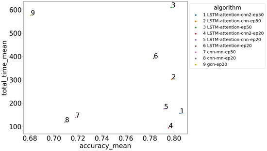
Figure 14. Execution time and accuracy for the neural classifiers.

Figure 15 shows the average accuracy and average execution time for the state-of-the-art neural classifiers.

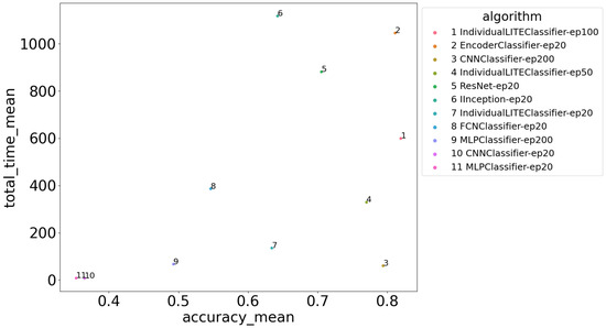
Figure 15. Execution time and accuracy for the state-of-the-art neural classifiers.

6.6. Multivariate Evaluation

We have chosen to reuse the windowing and dilation configurations that proved be the best in SCALE-BOSS-MR [15]. These are shown in Table 8 and Table 9.

Table 8. Window configurations.

Name	Window_Configs (Window Sizes)	Window Step
W0	24	1
W8	4, 8, 12, 16, 20, 24, 28, 32, 36, 40	1
W11	12, 16, 20, 24, 28, 32, 36, 40	4
W14	12, 16, 20, 24, 28, 32	2
W15	12, 16, 20, 24, 28, 32, 36, 40	8

Table 9. Dilation configurations.

Name	Dilation_Filter_Configs
D0	1 (no dilation)
D2	1, 7, 9, 11
D4	1, 11
D6	1, 9

The W0 configuration has a single window size with step 1, which is the baseline configuration. The W8 configuration has many window sizes with step 1; this configuration is the most compute-intensive but gave the best results in terms of accuracy in the SCALE-BOSS-MR case. The W11, W14 and W15 are very similar in terms of window size and the main difference is in the window step parameter.

Regarding dilation, larger dilation sizes mean that the algorithm can look further in time. Having multiple dilation sizes in theory gives the algorithm multiple resolution of the time-series. The D0 parameter is to have dilation 1 which means no dilation. This is the configuration that works as a baseline, to see the effects of dilation in the other configurations. D2 has the most dilation sizes (4 dilation sizes in total) aiming to provide the best accuracy. D4 and D6 have a single dilation size parameter beside 1.

In Table 10 we see the mean execution time and mean accuracy for the novel neural network architectures. As we can see, adding self-attention gives a 7 % boost in accuracy and that the STACK strategy is significantly more accurate compared to the BAG strategy.

Table 10. Proposed neural network methods’ mean accuracy and execution time.

	Accuracy_Mean	Accuracy_Pop_std	Total_Time_Mean	Total_Time_Pop_std
Algorithm
LSTM-attention-cnn2-ep50-stack	0.678	0.210	31.987	19.480
LSTM-CNN-ep50-stack	0.601	0.189	40.720	41.213
LSTM-attention-cnn2-ep50-bag	0.581	0.192	47.251	22.522
LSTM-CNN-ep20-stack	0.574	0.215	16.052	9.202
LSTM-attention-cnn2-ep20-stack	0.569	0.217	23.072	15.059
LSTM-attention-cnn2-ep20-bag	0.500	0.199	49.631	34.406

Table 11 provides the mean execution time and mean accuracy for the state-of-the-art neural networks. The CNNClassifier is really scalable and achieves good accuracy compared to other neural network methods. We can see that our proposed neural networks are significantly more accurate than the state-of-the-art classifiers.

Table 11. State-of-the-art neural network methods’ mean accuracy and execution time.

	Accuracy_Mean	Accuracy_Pop_std	Total_Time_Mean	Total_Time_Pop_std
Algorithm
EncoderClassifier-ep20	0.633	0.227	128.007	121.132
CNNClassifier-ep200	0.593	0.218	11.475	5.231
IInception-ep20	0.578	0.239	153.699	147.896
IndividualLITEClassifier-ep50	0.575	0.285	53.479	47.540
IndividualLITEClassifier-ep100	0.548	0.279	100.233	90.002
CNNClassifier-ep20	0.367	0.269	2.303	0.658
ResNet-ep20	0.299	0.154	103.053	101.543

In Table 12 we see the mean execution time and mean accuracy for the single window SCALE-BOSS-MR Multivariate (SBMR-MV).

Table 12. SCALE-BOSS-MR Multivariate (SBMR-MV) mean accuracy and execution time for a single window.

	Accuracy_Mean	Accuracy_Pop_std	Total_Time_Mean	Total_Time_Pop_std
Algorithm
SBMR-MV-ridge-cv-W0-trend-D2-BG-STACK	0.700	0.269	59.023	43.971
SBMR-MV-RF-W0-trend-D4-BG-STACK	0.691	0.216	29.784	22.312
SBMR-MV-ridge-cv-W0-trend-D4-BG-STACK	0.684	0.246	29.422	22.086
SBMR-MV-RF-W0-trend-D2-BG-STACK	0.684	0.237	59.453	44.198
SBMR-MV-ridge-cv-W0-trend-D2-BG-BAG	0.682	0.238	57.667	44.877
SBMR-MV-RF-W0-trend-D6-UG-STACK	0.667	0.239	26.334	20.425
SBMR-MV-RF-W0-trend-D0-UG-STACK	0.657	0.225	13.416	10.537
SBMR-MV-RF-W0-noTrend-D0-UG-STACK	0.650	0.192	6.987	5.445
SBMR-MV-RF-W0-trend-D2-BG-BAG	0.647	0.183	60.185	47.299
SBMR-MV-ridge-cv-W0-trend-D6-UG-BAG	0.646	0.230	25.831	20.542
SBMR-MV-ridge-cv-W0-trend-D4-BG-BAG	0.646	0.224	28.723	22.514
SBMR-MV-ridge-cv-W0-trend-D0-UG-STACK	0.643	0.226	13.293	10.460
SBMR-MV-RF-W0-trend-D4-BG-BAG	0.641	0.187	29.460	23.218
SBMR-MV-RF-W0-trend-D6-UG-BAG	0.637	0.194	27.080	21.417
SBMR-MV-RF-W0-trend-D0-UG-BAG	0.631	0.173	13.208	10.507
SBMR-MV-ridge-cv-W0-noTrend-D0-UG-STACK	0.629	0.227	6.847	5.475
SBMR-MV-ridge-cv-W0-trend-D0-UG-BAG	0.576	0.196	12.982	10.392
SBMR-MV-RF-W0-noTrend-D0-UG-BAG	0.571	0.170	6.870	5.493
SBMR-MV-ridge-cv-W0-noTrend-D0-UG-BAG	0.549	0.196	6.770	5.463

SBMR-MV-ridge-cv-W0-trend-D2-BG-STACK achieves the best accuracy but at the expense of execution time.

On the other hand, SBMR-MV-RF-W0-trend-D4-BG-STACK and SBMR-MV-ridge-cv-W0-trend-D4-BG-STACK achieve similar accuracy with significantly lower execution time. SBMR-MV-RF-W0-trend-D0-UG-STACK achieves an accuracy of 0.657 with a very low execution time. SBMR-MV-RF-W0-noTrend-D0-UG-STACK does not contain any trend information and gives an accuracy of 0.65. The above results show that adding trend information and dilation helps improve accuracy.

In Table 13 we see the mean execution time and mean accuracy for the multiple windows SBMR-MV. This table shows the effect of using multiple windows and chi squared test for feature selection and on top of dilation and trend information.

Table 13. SCALE-BOSS-MR Multivariate (SBMR-MV) mean accuracy and execution time for multiple windows.

	Accuracy_Mean	Accuracy_Pop_std	Total_Time_Mean	Total_Time_Pop_std
Algorithm
SBMR-MV-ridge-cv-W15-trend-D2-BG-BAG-chi	0.733	0.217	62.364	41.879
SBMR-MV-ridge-cv-W15-trend-D2-BG-STACK-chi	0.730	0.242	71.386	39.949
SBMR-MV-ridge-cv-W15-trend-D6-BG-STACK-chi	0.729	0.253	38.239	22.024
SBMR-MV-ridge-cv-W15-trend-D6-BG-BAG-chi	0.725	0.245	31.643	21.584
SBMR-MV-ridge-cv-W11-trend-D6-BG-STACK-chi	0.722	0.262	64.418	41.776
SBMR-MV-ridge-cv-W11-trend-D6-BG-BAG-chi	0.718	0.233	59.652	43.653
SBMR-MV-ridge-cv-W11-trend-D4-BG-STACK-chi	0.717	0.250	64.460	42.175
SBMR-MV-ridge-cv-W11-trend-D6-BG-STACK	0.717	0.268	67.959	41.675
SBMR-MV-ridge-cv-W15-trend-D4-BG-STACK-chi	0.715	0.251	35.160	20.303
SBMR-MV-ridge-cv-W15-trend-D6-BG-BAG	0.713	0.254	31.486	21.149
SBMR-MV-ridge-cv-W8-trend-D6-BG-STACK	0.713	0.263	298.052	210.282
SBMR-MV-ridge-cv-W15-trend-D6-BG-STACK	0.710	0.268	36.318	19.974
SBMR-MV-ridge-cv-W11-trend-D4-BG-BAG-chi	0.709	0.231	59.747	43.973
SBMR-MV-ridge-cv-W11-trend-D6-BG-BAG	0.708	0.253	75.683	56.347
SBMR-MV-ridge-cv-W14-trend-D6-BG-STACK	0.703	0.265	89.956	61.231
SBMR-MV-ridge-cv-W15-trend-D4-BG-BAG-chi	0.699	0.248	31.711	21.682
SBMR-MV-RF-W15-trend-D6-BG-STACK	0.698	0.213	37.453	20.296
SBMR-MV-ridge-cv-W8-trend-D6-BG-BAG	0.695	0.257	287.476	219.437
SBMR-MV-RF-W11-trend-D6-BG-BAG	0.687	0.201	59.510	42.949
SBMR-MV-RF-W11-trend-D6-BG-STACK	0.670	0.253	67.362	41.766
SBMR-MV-RF-W15-trend-D6-BG-BAG	0.651	0.188	32.324	21.439

SBMR-MV-ridge-cv-W15-trend-D2-BG-BAG-chi gives the best accuracy of 0.733 while being relatively scalable. SBMR-MV-ridge-cv-W15-trend-D2-BG-STACK-chi is not far behind but with higher execution time. SBMR-MV-ridge-cv-W15-trend-D6-BG-STACK-chi is also very close with accuracy 0.729 while being significantly more scalable compared to other window configurations. SBMR-MV-ridge-cv-W15-trend-D6-BG-BAG-chi is not far behind with accuracy of 0.725 while being even more scalable compared to SBMR-MV-ridge-cv-W15-trend-D6-BG-STACK-chi. SBMR-MV-ridge-cv-W15-trend-D6-BG-BAG achieves accuracy of 0.713, which shows that the chi squared test gives a slight bump in accuracy when using multiple windows.

We can also observe that the W15 configuration is generally better than W11 while also being significantly more scalable. W14 is not better than W11 or W15, neither in terms of performance nor in accuracy. W8 has by far the slowest execution time while not producing better results.

Table 12 and Table 13 answer RQ4 on how SCALE-BOSS-MR can be adapted to the multivariate use case and how it performs in terms of accuracy and execution time.

Table 14 shows the mean execution time and the mean accuracy for the Rocket family of classifiers. Both ROCKET and miniRocket proved to be very accurate, but ROCKET is significantly less scalable (in terms of execution time) than SBMR-MV.

Table 14. Rocket method mean accuracy and execution time.

	Accuracy_Mean	Accuracy_Pop_std	Total_Time_Mean	Total_Time_Pop_std
Algorithm
miniRocket	0.765	0.228	7.439	5.958
ROCKET	0.747	0.227	118.868	109.902

7. Conclusions

During our evaluation, we arrived at the following conclusions:

1.

The SCALE-BOSS-GRAPH algorithm proved very scalable, but its accuracy is lower than the state of the art.

2.

The GCNs were on par in terms of accuracy with the state-of-the-art deep learning methods, but were not that scalable compared to other methods.

3.

The proposed deep learning methods inspired by the text classification domain proved to be very effective both in terms of accuracy as well as in terms of execution time when compared with state-of-the-art deep learning methods both in the univariate and multivariate use cases. The optimizations we employed were instrumental for this result; for example, batch normalization gave a 5 % improvement in accuracy over the baseline, whereas adding an attention layer to the model gave a 10 % increase in accuracy but with a non-negligible cost in execution time. Adding convolutional layers to the architecture did not contribute much in accuracy but proved very beneficial in terms of execution time.

4.

The adaptation of SCALE-BOSS-MR to the multivariate use case namely SCALE-BOSS-MR-MV proved very scalable and accurate compared to the state of the art. More specifically, SCALE-BOSS-MR-MV proved to be more scalable than ROCKET while being marginally less accurate.

For future work, we plan to try transformer architectures fused with the SFA symbolic representation. Another line of research would be to try other Graph Neural Networks with more complex graph representations fused with the SFA symbolic representation.

References

- Chaovalitwongse, W.A.; Prokopyev, O.A.; Pardalos, P.M. Electroencephalogram (EEG) time series classification: Applications in epilepsy. Ann. Oper. Res. 2006, 148, 227–250. [Google Scholar] [CrossRef]
- Arul, M.; Kareem, A. Applications of shapelet transform to time series classification of earthquake, wind and wave data. Eng. Struct. 2021, 228, 111564. [Google Scholar] [CrossRef]
- Potamitis, I. Classifying insects on the fly. Ecol. Inform. 2014, 21, 40–49. [Google Scholar] [CrossRef]
- Susto, G.A.; Cenedese, A.; Terzi, M. Chapter 9—Time-Series Classification Methods: Review and Applications to Power Systems Data. In Big Data Application in Power Systems; Arghandeh, R., Zhou, Y., Eds.; Elsevier: Amsterdam, The Netherlands, 2018; pp. 179–220. [Google Scholar] [CrossRef]
- Ismail Fawaz, H.; Forestier, G.; Weber, J.; Idoumghar, L.; Muller, P.A. Evaluating surgical skills from kinematic data using convolutional neural networks. In Proceedings of the Medical Image Computing and Computer Assisted Intervention–MICCAI 2018: 21st International Conference, Granada, Spain, 16–20 September 2018; Proceedings, Part IV 11. Springer: Berlin/Heidelberg, Germany, 2018; pp. 214–221. [Google Scholar]
- Tao, L.; Elhamifar, E.; Khudanpur, S.; Hager, G.D.; Vidal, R. Sparse hidden markov models for surgical gesture classification and skill evaluation. In Proceedings of the Information Processing in Computer-Assisted Interventions: Third International Conference, IPCAI 2012, Pisa, Italy, 27 June 2012; Proceedings 3. Springer: Berlin/Heidelberg, Germany, 2012; pp. 167–177. [Google Scholar]
- Forestier, G.; Lalys, F.; Riffaud, L.; Trelhu, B.; Jannin, P. Classification of surgical processes using dynamic time warping. J. Biomed. Inform. 2012, 45, 255–264. [Google Scholar] [CrossRef]
- Devanne, M.; Wannous, H.; Berretti, S.; Pala, P.; Daoudi, M.; Del Bimbo, A. 3-D human action recognition by shape analysis of motion trajectories on riemannian manifold. IEEE Trans. Cybern. 2014, 45, 1340–1352. [Google Scholar] [CrossRef]
- Ji, S.; Xu, W.; Yang, M.; Yu, K. 3D convolutional neural networks for human action recognition. IEEE Trans. Pattern Anal. Mach. Intell. 2012, 35, 221–231. [Google Scholar] [CrossRef] [PubMed]
- Pinto, J.P.; Pimenta, A.; Novais, P. Deep learning and multivariate time series for cheat detection in video games. Mach. Learn. 2021, 110, 3037–3057. [Google Scholar] [CrossRef]
- Younis, R.; Zerr, S.; Ahmadi, Z. Multivariate time series analysis: An interpretable cnn-based model. In Proceedings of the 2022 IEEE 9th International Conference on Data Science and Advanced Analytics (DSAA), Shenzhen, China, 13–16 October 2022; IEEE: Piscataway Township, NJ, USA, 2022; pp. 1–10. [Google Scholar]
- Madrid, F.; Singh, S.; Chesnais, Q.; Mauck, K.; Keogh, E. Matrix profile xvi: Efficient and effective labeling of massive time series archives. In Proceedings of the 2019 IEEE International Conference on Data Science and Advanced Analytics (DSAA), Washington, DC, USA, 5–8 October 2019; IEEE: Piscataway Township, NJ, USA, 2019; pp. 463–472. [Google Scholar]
- Devanne, M.; Rémy-Néris, O.; Le Gals-Garnett, B.; Kermarrec, G.; Thepaut, A. A co-design approach for a rehabilitation robot coach for physical rehabilitation based on the error classification of motion errors. In Proceedings of the 2018 Second IEEE International Conference on Robotic Computing (IRC), Laguna Hills, CA, USA, 31 January–2 February 2018; IEEE: Piscataway Township, NJ, USA, 2018; pp. 352–357. [Google Scholar]
- Schäfer, P.; Högqvist, M. SFA: A symbolic fourier approximation and index for similarity search in high dimensional datasets. In Proceedings of the 15th International Conference on Extending Database Technology, Berlin, Germany, 27–30 March 2012; ACM: New York, NY, USA, 2012; pp. 516–527. [Google Scholar]
- Glenis, A.; Vouros, G.A. SCALE-BOSS-MR: Scalable Time Series Classification Using Multiple Symbolic Representations. Appl. Sci. 2024, 14, 689. [Google Scholar] [CrossRef]
- Lin, J.; Keogh, E.; Wei, L.; Lonardi, S. Experiencing SAX: A novel symbolic representation of time series. Data Min. Knowl. Discov. 2007, 15, 107–144. [Google Scholar] [CrossRef]
- Senin, P.; Malinchik, S. Sax-vsm: Interpretable time series classification using sax and vector space model. In Proceedings of the 2013 IEEE 13th International Conference on Data Mining, Dallas, TX, USA, 7–10 December 2013; IEEE: Piscataway Township, NJ, USA, 2013; pp. 1175–1180. [Google Scholar]
- Schäfer, P. The BOSS is concerned with time series classification in the presence of noise. Data Min. Knowl. Discov. 2015, 29, 1505–1530. [Google Scholar] [CrossRef]
- Schäfer, P. Scalable time series classification. Data Min. Knowl. Discov. 2016, 30, 1273–1298. [Google Scholar]
- Schäfer, P.; Leser, U. Fast and accurate time series classification with weasel. In Proceedings of the 2017 ACM on Conference on Information and Knowledge Management, Singapore, 6–10 November 2017; ACM: New York, NY, USA, 2017; pp. 637–646. [Google Scholar]
- Glenis, A.; Vouros, G.A. Balancing between scalability and accuracy in time-series classification for stream and batch settings. In Proceedings of the Discovery Science: 23rd International Conference, DS 2020, Thessaloniki, Greece, 19–21 October 2020; Proceedings 23. Springer: Berlin/Heidelberg, Germany, 2020; pp. 265–279. [Google Scholar]
- Nguyen, T.L.; Ifrim, G. MrSQM: Fast time series classification with symbolic representations. arXiv 2021, arXiv:2109.01036. [Google Scholar]
- Nguyen, T.L.; Ifrim, G. Fast time series classification with random symbolic subsequences. In Proceedings of the International Workshop on Advanced Analytics and Learning on Temporal Data, Grenoble, France, 19–23 September 2022; Springer: Berlin/Heidelberg, Germany, 2022; pp. 50–65. [Google Scholar]
- Glenis, A.; Vouros, G.A. SCALE-BOSS: A framework for scalable time-series classification using symbolic representations. In Proceedings of the 12th Hellenic Conference on Artificial Intelligence, Corfu, Greece, 7–9 September 2022; pp. 1–9. [Google Scholar]
- Schäfer, P.; Leser, U. WEASEL 2.0–A Random Dilated Dictionary Transform for Fast, Accurate and Memory Constrained Time Series Classification. arXiv 2023, arXiv:2301.10194. [Google Scholar]
- Schäfer, P.; Leser, U. Multivariate time series classification with WEASEL+ MUSE. arXiv 2017, arXiv:1711.11343. [Google Scholar]
- Dempster, A.; Petitjean, F.; Webb, G.I. ROCKET: Exceptionally fast and accurate time series classification using random convolutional kernels. Data Min. Knowl. Discov. 2020, 34, 1454–1495. [Google Scholar] [CrossRef]
- Dempster, A.; Schmidt, D.F.; Webb, G.I. Minirocket: A very fast (almost) deterministic transform for time series classification. In Proceedings of the 27th ACM SIGKDD Conference on Knowledge Discovery & Data Mining, Singapore, 14–18 August 2021; pp. 248–257. [Google Scholar]
- Wang, Z.; Yan, W.; Oates, T. Time series classification from scratch with deep neural networks: A strong baseline. In Proceedings of the 2017 International Joint Conference on Neural Networks (IJCNN), Anchorage, AK, USA, 14–19 May 2017; IEEE: Piscataway Township, NJ, USA, 2017; pp. 1578–1585. [Google Scholar]
- Srivastava, N.; Hinton, G.; Krizhevsky, A.; Sutskever, I.; Salakhutdinov, R. Dropout: A simple way to prevent neural networks from overfitting. J. Mach. Learn. Res. 2014, 15, 1929–1958. [Google Scholar]
- Nair, V.; Hinton, G.E. Rectified linear units improve restricted boltzmann machines. In Proceedings of the 27th International Conference on Machine Learning (ICML-10), Haifa, Israel, 21–24 June 2010; pp. 807–814. [Google Scholar]
- Ioffe, S. Batch normalization: Accelerating deep network training by reducing internal covariate shift. arXiv 2015, arXiv:1502.03167. [Google Scholar] [CrossRef]
- He, K.; Zhang, X.; Ren, S.; Sun, J. Deep residual learning for image recognition. In Proceedings of the IEEE Conference on Computer Vision and Pattern Recognition, Las Vegas, NV, USA, 27–30 June 2016; pp. 770–778. [Google Scholar]
- Monti, F.; Frasca, F.; Eynard, D.; Mannion, D.; Bronstein, M.M. Fake news detection on social media using geometric deep learning. arXiv 2019, arXiv:1902.06673. [Google Scholar] [CrossRef]
- Zhao, B.; Lu, H.; Chen, S.; Liu, J.; Wu, D. Convolutional neural networks for time series classification. J. Syst. Eng. Electron. 2017, 28, 162–169. [Google Scholar] [CrossRef]
- Serra, J.; Pascual, S.; Karatzoglou, A. Towards a universal neural network encoder for time series. In Artificial Intelligence Research and Development; IOS Press: Amsterdam, The Netherlands, 2018; pp. 120–129. [Google Scholar]
- Ismail Fawaz, H.; Lucas, B.; Forestier, G.; Pelletier, C.; Schmidt, D.F.; Weber, J.; Webb, G.I.; Idoumghar, L.; Muller, P.A.; Petitjean, F. Inceptiontime: Finding alexnet for time series classification. Data Min. Knowl. Discov. 2020, 34, 1936–1962. [Google Scholar] [CrossRef]
- Ismail-Fawaz, A.; Devanne, M.; Weber, J.; Forestier, G. Deep learning for time series classification using new hand-crafted convolution filters. In Proceedings of the 2022 IEEE International Conference on Big Data (Big Data), Osaka, Japan, 17–20 December 2022; IEEE: Piscataway Township, NJ, USA, 2022; pp. 972–981. [Google Scholar]
- Ismail-Fawaz, A.; Devanne, M.; Berretti, S.; Weber, J.; Forestier, G. Lite: Light inception with boosting techniques for time series classification. In Proceedings of the 2023 IEEE 10th International Conference on Data Science and Advanced Analytics (DSAA), Thessaloniki, Greece, 9–13 October 2023; IEEE: Piscataway Township, NJ, USA, 2023; pp. 1–10. [Google Scholar]
- Cui, Z.; Chen, W.; Chen, Y. Multi-scale convolutional neural networks for time series classification. arXiv 2016, arXiv:1603.06995. [Google Scholar] [CrossRef]
- Wickstrøm, K.; Kampffmeyer, M.; Mikalsen, K.Ø.; Jenssen, R. Mixing up contrastive learning: Self-supervised representation learning for time series. Pattern Recognit. Lett. 2022, 155, 54–61. [Google Scholar] [CrossRef]
- Ordonez, P.; Armstrong, T.; Oates, T.; Fackler, J. Using modified multivariate bag-of-words models to classify physiological data. In Proceedings of the 2011 IEEE 11th International Conference on Data Mining Workshops, Vancouver, BC, Canada, 11 December 2011; IEEE: Piscataway Township, NJ, USA, 2011; pp. 534–539. [Google Scholar]
- Baydogan, M.G.; Runger, G. Learning a symbolic representation for multivariate time series classification. Data Min. Knowl. Discov. 2015, 29, 400–422. [Google Scholar] [CrossRef]
- Ruiz, A.P.; Flynn, M.; Large, J.; Middlehurst, M.; Bagnall, A. The great multivariate time series classification bake off: A review and experimental evaluation of recent algorithmic advances. Data Min. Knowl. Discov. 2021, 35, 401–449. [Google Scholar] [CrossRef] [PubMed]
- Shervashidze, N.; Schweitzer, P.; Van Leeuwen, E.J.; Mehlhorn, K.; Borgwardt, K.M. Weisfeiler-Lehman graph kernels. J. Mach. Learn. Res. 2011, 12, 2539–2561. [Google Scholar]
- LeCun, Y. Generalization and network design strategies. Connect. Perspect. 1989, 19, 18. [Google Scholar]
- LeCun, Y.; Bengio, Y. Convolutional networks for images, speech, and time series. Handb. Brain Theory Neural Netw. 1995, 3361, 1995. [Google Scholar]
- Rumelhart, D.E.; Hinton, G.E.; Williams, R.J. Learning Internal Representations by Error Propagation. In Parallel Distributed Processing: Explorations in the Microstructure of Cognition, Vol. 1: Foundations; MIT Press: Cambridge, MA, USA, 1986; pp. 318–362. [Google Scholar]
- Elman, J.L. Finding structure in time. Cogn. Sci. 1990, 14, 179–211. [Google Scholar] [CrossRef]
- Jordan, M.I. Serial order: A parallel distributed processing approach. In Advances in Psychology; Elsevier: Amsterdam, The Netherlands, 1997; Volume 121, pp. 471–495. [Google Scholar]
- Hochreiter, S.; Schmidhuber, J. Long short-term memory. Neural Comput. 1997, 9, 1735–1780. [Google Scholar] [CrossRef]
- Bahdanau, D.; Cho, K.; Bengio, Y. Neural machine translation by jointly learning to align and translate. arXiv 2014, arXiv:1409.0473. [Google Scholar]
- Sugiyama, M.; Borgwardt, K. Halting in random walk kernels. Adv. Neural Inf. Process. Syst. 2015, 28, 1639–1647. [Google Scholar]
- Faouzi, J.; Janati, H. pyts: A Python Package for Time Series Classification. J. Mach. Learn. Res. 2020, 21, 1–6. [Google Scholar]
- Siglidis, G.; Nikolentzos, G.; Limnios, S.; Giatsidis, C.; Skianis, K.; Vazirgiannis, M. Grakel: A graph kernel library in python. J. Mach. Learn. Res. 2020, 21, 1–5. [Google Scholar]
- Pedregosa, F.; Varoquaux, G.; Gramfort, A.; Michel, V.; Thirion, B.; Grisel, O.; Blondel, M.; Prettenhofer, P.; Weiss, R.; Dubourg, V.; et al. Scikit-learn: Machine learning in Python. J. Mach. Learn. Res. 2011, 12, 2825–2830. [Google Scholar]
- Chollet, F. Deep Learning with Python; Simon and Schuster: New York, NY, USA, 2021. [Google Scholar]
- Data61, C. StellarGraph Machine Learning Library. 2018. Available online: https://github.com/stellargraph/stellargraph (accessed on 9 September 2025).
- Dau, H.A.; Bagnall, A.; Kamgar, K.; Yeh, C.C.M.; Zhu, Y.; Gharghabi, S.; Ratanamahatana, C.A.; Keogh, E. The UCR time series archive. IEEE/CAA J. Autom. Sin. 2019, 6, 1293–1305. [Google Scholar] [CrossRef]
- Middlehurst, M.; Ismail-Fawaz, A.; Guillaume, A.; Holder, C.; Guijo-Rubio, D.; Bulatova, G.; Tsaprounis, L.; Mentel, L.; Walter, M.; Schäfer, P.; et al. aeon: A Python toolkit for learning from time series. J. Mach. Learn. Res. 2024, 25, 1–10. [Google Scholar]
Disclaimer/Publisher’s Note: The statements, opinions and data contained in all publications are solely those of the individual author(s) and contributor(s) and not of MDPI and/or the editor(s). MDPI and/or the editor(s) disclaim responsibility for any injury to people or property resulting from any ideas, methods, instructions or products referred to in the content. |
© 2025 by the authors. Licensee MDPI, Basel, Switzerland. This article is an open access article distributed under the terms and conditions of the Creative Commons Attribution (CC BY) license (https://creativecommons.org/licenses/by/4.0/).