A Comparative Evaluation of Time-Series Forecasting Models for Energy Datasets

Abstract

Time series forecasting plays a critical role across numerous domains such as finance, energy, and healthcare. While traditional statistical models have long been employed for this task, recent advancements in deep learning have led to a new generation of state-of-the-art (SotA) models that offer improved accuracy and flexibility. However, there remains a gap in understanding how these forecasting models perform under different forecasting scenarios, especially when incorporating external variables. This paper presents a comprehensive review and empirical evaluation of seven leading deep learning models for time series forecasting. We introduce a novel dataset that combines energy consumption and weather data from 24 European countries, allowing us to benchmark model performance across various forecasting horizons, granularities, and variable types. Our findings offer practical insights into model strengths and limitations, guiding future applications and research in time series forecasting.

1. Introduction

Time series forecasting is a foundational task in numerous domains, including finance, energy, healthcare, and environmental monitoring. By analyzing historical, time-ordered data, forecasting models enable decision-makers to anticipate future trends, detect patterns, and optimize planning [1]. The increasing availability of large, complex datasets has amplified the need for accurate and robust forecasting methods capable of handling diverse and dynamic real-world conditions.

Traditional statistical methods such as ARIMA [2] and Exponential Smoothing have long served as reliable tools for time series forecasting, particularly in univariate settings. However, these approaches often struggle to capture non-linear relationships, long-term dependencies, and interactions between multiple variables.

The advent of deep learning has transformed the landscape of time series forecasting. Neural network architectures like Recurrent Neural Networks (RNNs) [3], Long Short-Term Memory (LSTM) networks [4], and Gated Recurrent Units (GRUs) have shown strong performance in capturing complex temporal dynamics. More recent innovations, such as Convolutional Neural Networks (CNNs) [5], transformer-based models [6], and Graph Neural Networks (GNNs) [7], further enhance the ability to model both local patterns and long-range dependencies in time series data. Similar advancements in deep learning have also been effectively applied in related domains such as landslide detection, remote sensing object recognition, and cross-view person search, further demonstrating the versatility of neural models in complex spatial and contextual environments [8,9,10].

Time series forecasting tasks can vary widely in scope and complexity:

• Univariate forecasting involves predicting future values based solely on the past observations of a single variable. This is common in applications like temperature or electricity demand forecasting.
• Multivariate forecasting uses multiple interrelated time series as inputs, allowing models to capture dependencies across variables, such as combining energy consumption and weather data.
• Short-term forecasting targets near-future predictions (e.g., the next few hours or days), where recent patterns are critical.
• Long-term forecasting involves predictions over extended periods (weeks or months), requiring models to learn more persistent trends and seasonalities.
• Exogenous variables, are external inputs that help predict a target variable. These variables are not predicted themselves—they are assumed to be known or fixed for the forecast horizon. Exogenous variables can be time series (e.g., weather) or static/categorical (e.g., day of the week, holiday indicators). They provide contextual information, enriching the model’s understanding of factors influencing the target.

Deep learning models such as N-BEATS, N-HiTS, Autoformer, and others are designed to tackle these challenges by automatically extracting relevant features and modeling intricate temporal relationships. Some models, like NBEATSx [11] and Prophet [12], are specifically built to incorporate exogenous variables effectively.

In this study, we evaluate seven state-of-the-art deep learning models using a novel dataset comprising electricity consumption and weather data from 24 European countries. Our evaluation framework is designed to assess model performance across multiple dimensions: univariate vs. multivariate forecasting, short-term vs. long-term horizons, and their combinations. By systematically analyzing these models in real-world-like settings, we aim to identify their strengths, limitations, and practical applicability.

The rest of this paper is organized as follows: Section 2 presents related work. Section 3 provides an overview of the selected models. Section 4 describes the dataset, experimental setup, and evaluation metrics. Section 5 presents the results. Section 6 concludes the paper and discusses potential future directions.

2. Related Work

Recent years have seen rapid growth in the development of deep learning models tailored for time series forecasting [13,14,15]. Traditional models such as ARIMA, SARIMA, and Holt–Winters have historically dominated the field due to their interpretability and statistical rigor [16,17]. However, these models often struggle with non-linear dependencies and complex multivariate relationships.

Deep learning methods began gaining traction with the introduction of Recurrent Neural Networks (RNNs) [18], particularly Long Short-Term Memory (LSTM) networks [19,20,21], which were designed to model long-range temporal dependencies. Subsequent innovations like GRUs and attention mechanisms further improved sequence modeling capabilities. More recently, transformer-based models, originally developed for natural language processing, have demonstrated significant promise in handling long time-series sequences due to their parallelization and global receptive fields [22,23].

Several comparative studies have attempted to benchmark these models across public datasets such as M4, ETT, and ElectricityLoadDiagrams. However, these datasets often lack the complexity and granularity found in real-world applications. Moreover, many evaluations focus solely on accuracy, overlooking computational efficiency and the impact of exogenous variables.

Our work builds on these foundations by offering a more holistic evaluation using a novel and diverse dataset that reflects real-world energy usage patterns. We explore both predictive accuracy and operational aspects such as memory usage and training time, and we specifically assess model performance with and without exogenous input data.

3. Models Reviewed

The selection of the seven models evaluated in this study—NBEATS, NBEATSx, NHITS, DLinear, Autoformer, Informer, and FEDformer—was guided by their consistent performance as state-of-the-art approaches in the recent time series forecasting literature. These models have frequently been benchmarked against one another across major forecasting competitions and empirical studies, demonstrating robust accuracy and scalability. By focusing on this subset, we ensure a fair and meaningful comparison among top-performing architectures that represent both classical deep learning paradigms and modern transformer-based designs. Importantly, all evaluated models are easily accessible through the neuralforecast https://pypi.org/project/neuralforecast (accessed on 20 June 2025) library [24].

3.1. N-BEATS and NBEATSx

Neural Basis Expansion Analysis for Time-Series (N-BEATS) [25] is a deep-learning model designed for univariate time series forecasting. It employs linear projections, fully connected layers, basis functions, and a doubly residual stacking mechanism, which collectively contribute to its state-of-the-art performance. By further refining the model’s structure, it is possible to identify trends and seasonality components, thereby enhancing the model’s interpretability. NBEATSx is an extension model of N-BEATS that can incorporate time-dependent and static exogenous factors. This addition can help the model to integrate useful information resulting in better performance. Both models were developed to eschew traditional time-series feature engineering, instead leveraging deep learning capabilities to uncover hidden patterns within the data.

3.2. N-HiTS

Neural Hierarchical Interpolation for Time Series (N-HiTS) [26] is based on N-BEATS’s structure. In addition, it incorporates multi-rate data sampling and hierarchical interpolation intending to enhance accuracy, particularly in long-horizon time series forecasting tasks. By adding sub-sampling layers in front of fully connected blocks, the computational cost is reduced but the ability of modeling long-rage dependencies is preserved. Hierarchical interpolation provides smoothness in predictions by reducing the dimensionality. With a unique structure, N-HiTS combines these two aspects achieving each block to specialize in forecasting its own frequency band of the time-series signal. N-HiTS has the best results on long-term forecasting tasks and outperforms all transformer models while requiring less computational power.

3.3. DLinear

DLinear is a lightweight deep learning model designed for efficient and accurate time series forecasting. Its core idea is to separate the time series into trend and seasonal components using a decomposition-based approach, and then model each component using simple linear projections. This decomposition allows the model to focus on learning individual behaviors more effectively while maintaining computational efficiency. Unlike complex architectures that rely on attention or deep stacking, DLinear uses straightforward linear layers, making it highly scalable and resource-efficient. Its simplicity not only reduces the risk of overfitting but also enables faster training and lower memory usage, which is particularly beneficial in large-scale or low-latency applications. Despite its minimalistic design, DLinear has demonstrated competitive accuracy across several benchmarks and has become a strong baseline for time series forecasting, as highlighted in recent comparative evaluations of transformer-based and linear models [27].

3.4. Autoformer

Over the past few years, advancements in transformer models have significantly reshaped the landscape of natural language processing (NLP) and artificial intelligence (AI). These models not only exhibit superior performance in traditional NLP benchmarks but also demonstrate transformative potential in real-world applications. This is the reason that it did not take too long for the first time-series version of the transformer to be created. Autoformer [28] as a transformer model has an encoder and a decoder, and instead of the classic attention, it utilizes the auto-correlation mechanism. The auto-correlation mechanism that is used on the encoder focuses on the seasonal part modeling, while on the decoder, there is an extra accumulated structure for trend-cyclical components as well. Autoformer achieves better results on long-term forecasting in both univariate and multivariate cases.

3.5. Informer

Informer [29] is a transformer-based model specifically designed to improve computational efficiency and scalability in long sequence time series forecasting. Its primary innovation lies in the introduction of the ProbSparse self-attention mechanism, which significantly reduces the computational cost by focusing attention on a subset of “informative” queries. This probabilistic sparsity technique prioritizes high-impact time steps while discarding redundant ones, thereby preserving performance while enhancing speed and memory efficiency. Unlike traditional transformer decoders, Informer adopts a generative-style decoder, which produces multi-step forecasts in a single forward pass, rather than autoregressively. These design choices enable Informer to outperform many earlier models in both univariate and multivariate scenarios with substantially lower resource demands.

3.6. FEDformer

The Frequency Enhanced Decomposition Transformer (FEDformer) [30] introduces a fundamentally different architectural approach compared to Informer. Rather than relying on attention mechanisms, FEDformer integrates Fourier and Wavelet transforms to analyze and forecast time series in the frequency domain. Specifically, it replaces conventional self-attention with frequency-enhanced blocks that decompose the input into seasonal and trend components, capturing global temporal patterns more effectively. This frequency-based decomposition allows the model to handle long-term dependencies without the quadratic overhead of attention. Furthermore, by selecting a fixed number of Fourier bases, FEDformer reduces the computational and memory footprint to linear complexity while maintaining high predictive performance. While both models aim to address the inefficiencies of classical transformer models for time series, they take fundamentally different paths: Informer uses a sparse attention strategy in the time domain, whereas FEDformer emphasizes frequency-domain transformations to extract long-term structures.

4. Dataset Description

In this review article, we explore SotA deep neural networks specifically designed for time series forecasting. Traditionally, the efficacy of these models has been validated using pre-existing datasets, often leading to results that might not fully capture the models’ capabilities across diverse and practical scenarios. To address this limitation and ensure a more comprehensive evaluation, we have compiled a novel collection of datasets. This dataset comprises energy consumption data from 24 European countries, sourced from the European Network of Transmission System Operators for Electricity (ENTSO-E) https://www.entsoe.eu/ (accessed on 20 June 2025). The data is characterized by varying levels of granularity, providing a robust test for examining model performance across different temporal resolutions.

Additionally, to enhance the richness of our dataset and enable the deep learning models to capture more intricate patterns, we have integrated corresponding weather data for each country. This auxiliary data introduces additional contextual information that can be critical for accurately modeling and forecasting energy consumption trends, especially given the influence of weather on energy usage. By leveraging this multi-faceted dataset, we aim to provide a more objective and holistic assessment of the capabilities of contemporary deep neural network models in the realm of time series forecasting. Weather data are sourced from Open-Meteo https://open-meteo.com/ (accessed on 20 June 2025) platform [31].

As shown in

Table 1. Key columns in the energy–weather time series dataset (bold: features used in multivariate forecasting).

Column Name	Description
Time (UTC)	Forecast time interval in UTC format
TIME_LOCAL	Local timestamp adjusted to time zone
Day-ahead Total Load Forecast [MW]	Forecasted energy demand (dropped during preprocessing)
Actual Total Load [MW]	Actual recorded energy demand (target variable)
weathercode (wmo code)	Encoded weather condition (not used)
temperature_2m_max (°C)	Daily maximum temperature
temperature_2m_min (°C)	Daily minimum temperature
temperature_2m_mean (°C)	Daily mean temperature
apparent_temperature_max (°C)	Feels-like max temperature
apparent_temperature_min (°C)	Feels-like min temperature
apparent_temperature_mean (°C)	Feels-like mean temperature
sunrise/sunset (iso8601)	Sunrise and sunset times (not used)
precipitation (mm)	Total daily precipitation
rain (mm)	Rainfall volume
snowfall (cm)	Snow accumulation
precipitation_hours (h)	Hours of precipitation
windspeed_10m_max (km/h)	Max wind speed at 10m
windgusts_10m_max (km/h)	Peak wind gusts
winddirection_10m_dominant (°B)	Dominant wind direction
shortwave_radiation (MJ/mB²)	Incoming solar radiation
et0_fao_evapotranspiration (mm)	FAO-56 evapotranspiration reference

, the dataset developed for this study integrates energy consumption and weather data, offering a rich and multidimensional resource for time series forecasting. Each record includes 24 columns capturing both temporal and contextual features. The energy-related fields consist of Time (UTC), TIME_LOCAL, Day-ahead Total Load Forecast [MW], and Actual Total Load [MW], providing both predicted and real-time load values with high-frequency resolution (e.g., 15-min intervals). Temporal features include standardized date and time formats, such as ISO8601 timestamps [32].

The dataset also incorporates extensive meteorological variables, including maximum, minimum, and mean values for both actual and apparent temperatures, along with precipitation metrics (precipitation, rain, snowfall, and precipitation_hours). Additional features such as wind speed, wind gusts, dominant wind direction, shortwave radiation, and evapotranspiration are included to capture weather phenomena that influence energy demand. Sunrise and sunset timestamps are also provided to allow modeling of solar cycles.

This comprehensive set of features enables the dataset to support both univariate and multivariate forecasting experiments, as well as models utilizing exogenous variables. To promote reproducibility and facilitate future research, the necessary code and datasets used in this study are publicly available on GitHub https://github.com/NikitasMaragkos (accessed on 20 June 2025) under the Creative Commons Attribution-NonCommercial-ShareAlike 4.0 International License https://creativecommons.org/licenses/by-nc-sa/4.0/ (accessed on 20 June 2025).

5. Experimental Setup

To provide a thorough assessment of the SotA deep neural networks for time series forecasting, we established a multi-faceted comparative evaluation framework. This framework is designed to rigorously test each model across a variety of scenarios, reflecting different real-world forecasting challenges and data characteristics.

We structured our comparisons around several key scenarios to evaluate the versatility and robustness of each model:

Univariate vs. Multivariate Forecasting

Univariate Forecasting: We tested the models on datasets containing a single variable, such as energy consumption for a single country.

Multivariate Forecasting: We expanded the scope to include multiple interrelated variables, like energy consumption combined with weather data across multiple countries.

Forecasting Horizons

Short-Term Forecasting: We evaluated model performance on tasks requiring predictions over short periods (e.g., next few hours or days).

Long-Term Forecasting: The models were also tested on long-term forecasting tasks, where the prediction spans extended to weeks or months ahead.

In combination with the aggregations, which are hourly, daily, and monthly, we can see in

Table 2. Forecasting horizons used in each aggregation and time span.

Forecast Type	Hourly	Daily	Monthly
Short-Term	24 h	2 days	2 months
Long-Term	168 h	365 days	12 months

the corresponding horizons.

5.1. Hyperparameter Selection and Model Transfer Strategy

To efficiently evaluate a wide range of forecasting models across multiple European countries, we adopted a two-stage experimental strategy designed to balance computational feasibility with rigorous model selection.

In the first stage, we performed an extensive hyperparameter search using data from Belgium, which was chosen as a representative country due to its diverse seasonal and load characteristics. For each model, we explored a broad set of hyperparameter combinations under different temporal aggregation levels (hourly, daily, and monthly) and forecasting horizons. All experiments in this stage were conducted in a univariate setting, using only the target variable (i.e., actual energy load) to ensure a controlled and consistent basis for evaluation.

Following the initial grid search, we selected the top 10 configurations per model based on validation performance, representing the most promising setups for the univariate case. To ensure robust hyperparameter selection and avoid overfitting to the characteristics of a single country, we additionally included 10 configurations randomly sampled from the entire search space. This strategy increases diversity and mitigates dataset-specific bias, ensuring broader coverage of the hyperparameter landscape. As a result, a pool of 20 candidate configurations per model was formed, enhancing generalization and supporting fair comparative evaluation across all countries.

In the second stage, we applied these 20 scenarios to all other countries in our dataset. Each configuration was evaluated using training and validation splits specific to the respective country’s data, allowing for performance benchmarking across diverse regions. This transfer approach enables us to assess how well hyperparameters tuned in one region generalize to others, offering insights into model robustness and cross-country adaptability.

It is important to note that all initial experiments, that concluded in the 20 scenarios, were performed under a univariate modeling framework. For all cases, MinMax scaling was applied to the data for better training results after several experiments with various scaling techniques.

5.2. Evaluation Metrics

To gauge the models’ effectiveness, we utilized a comprehensive set of performance metrics tailored to different aspects of forecasting.

Main Metric

We employed the Mean Absolute Percentage Error (MAPE) as the primary metric to evaluate forecasting accuracy. MAPE offers an intuitive interpretation by expressing prediction errors as a percentage of the actual values, which facilitates comparison across different countries and aggregation levels regardless of the scale of electricity demand. This scale-independence is particularly valuable in our study, where energy consumption varies significantly between countries. Furthermore, MAPE is widely used in both academic literature and industry practice, making it a suitable choice for benchmarking and ensuring the relevance and interpretability of our results.

Computational Efficiency

In addition to accuracy, we considered the computational efficiency of each model. Specifically, we evaluated the following:

• Training Time: The duration required to train each model was recorded, highlighting the trade-offs between speed and forecasting performance.
• Memory Usage: The memory consumed during training and inference was monitored to assess the computational resources each model demands.

Comparative Analysis

By evaluating each model across these diverse dimensions, we aimed to uncover strengths and limitations specific to different types of time series forecasting tasks. This comprehensive approach not only highlights the predictive accuracy of the models but also provides a detailed understanding of their operational efficiency and suitability for various practical applications.

5.3. Experimental Results

5.3.1. Univariate vs. Multivariate Forecasting

To investigate the comparative performance of univariate and multivariate forecasting models, we analyzed their effectiveness across multiple temporal aggregation levels (hourly, daily, and monthly) and countries. Overall, univariate models outperformed multivariate models in 55.53% of all cases. This trend was especially strong in models such as DLinear (71.74% on hourly data) and NBEATS (70.83% on hourly data), indicating their robustness in scenarios where incorporating external variables may introduce noise rather than predictive gain. This pattern is clearly illustrated in

Table 3. Percentage of cases where univariate models outperform multivariate models. The cases where multivariate models are better, are bold.

Model	Hourly (H)	Daily (D)	Monthly (M)
AUTOFORMER	60.42%	50.00%	60.42%
NBEATS	70.83%	66.67%	54.17%
NHITS	65.22%	54.17%	47.92%
DLINEAR	71.74%	60.42%	62.50%
INFORMER	41.67%	41.67%	47.92%
FEDFORMER	42.55%	50.00%	52.08%
Overall	55.53% of cases favor univariate models

, which shows the percentage of cases where univariate models outperform multivariate ones across different architectures and aggregation levels.

However, this dominance was not uniform across all models. Transformer-based architectures like Informer and FEDformer showed better performance in the multivariate setting, particularly on hourly and daily resolutions. Specifically, Informer achieved higher accuracy with multivariate inputs in 58.33% of hourly and daily cases, suggesting these models are better equipped to exploit complex dependencies between energy demand and weather features. Interestingly, the NHITS model showed a reversal in monthly aggregation, where multivariate input outperformed univariate in 52.08% of cases. This suggests that long-term forecasting may benefit more from enriched contextual data, especially when temporal patterns become coarser and external influences more pronounced.

These findings highlight that the advantage of multivariate modeling is architecture-dependent. As shown in Table 3, transformer-based models such as Informer and FEDformer demonstrate strong performance in multivariate scenarios, particularly in hourly and daily forecasting tasks. This suggests that, under appropriate configurations and data scales, transformers are capable of effectively capturing long-range dependencies and complex variable interactions. In contrast, models like DLinear and NBEATS, which rely on simpler or decomposition-based architectures, tend to perform better in univariate settings—likely due to their reduced sensitivity to noisy or redundant external features. These patterns imply that model selection should be guided not only by the task but also by the architecture’s ability to balance complexity and generalization.

5.3.2. Memory and Training Time

Table 4. Relative time and memory usage of forecasting models (DLINEAR as baseline).

Model	Time Multiplier	Memory Multiplier
DLINEAR	1.00	1.00
NBEATS	1.28	0.79
NHITS	2.38	1.13
AUTOFORMER	54.98	87.88
FEDFORMER	103.80	20.86
INFORMER	95.58	19.67

provides a comparative overview of training time and memory consumption for each forecasting model, normalized relative to DLINEAR, which is the most lightweight model in the study. DLINEAR, with a multiplier of 1.0 in both dimensions, serves as the baseline for evaluating the computational efficiency of the other models.

The results highlight a clear distinction between classical deep learning models and transformer-based architectures. NBEATS and NHITS demonstrate only modest increases in resource requirements, consuming approximately 1.3× to 2.4× more time and marginally more memory than DLINEAR. These models offer a favorable balance between computational cost and modeling capability, making them suitable for moderately constrained environments.

In contrast, transformer-based models such as AUTOFORMER, FEDFORMER, and INFORMER exhibit significantly higher training times and memory demands. Specifically, FEDFORMER and INFORMER require over 100× the training time and more than 20× the memory of DLINEAR. AUTOFORMER, while even more memory-intensive, achieves similar time costs. These models, while potentially offering higher predictive accuracy, are best suited for offline training settings or high-performance computing environments due to their substantial resource footprint.

This analysis underscores the importance of considering computational efficiency when selecting forecasting models for practical deployment, especially in energy-constrained or real-time scenarios.

5.3.3. Best Models

In the final evaluation step, we assessed all models across all combinations of forecasting horizons and temporal aggregation levels. The following observations highlight the top-performing models in each scenario.

Hourly Aggregation—Short-Term Forecasting

In this setting (Figure 1), the Informer model leads with a 41.6% win rate. Its performance is equally split between the univariate and multivariate configurations (each at 20.8%). NBEATS follows, with 20.8% of wins attributed to its univariate form and an additional 4.2% to its multivariate variant. NHITS and DLinear round out the top-performing models in this scenario. These results demonstrate the strength of transformer-based architectures in short-term, high-resolution forecasting, particularly when temporal dependencies dominate.

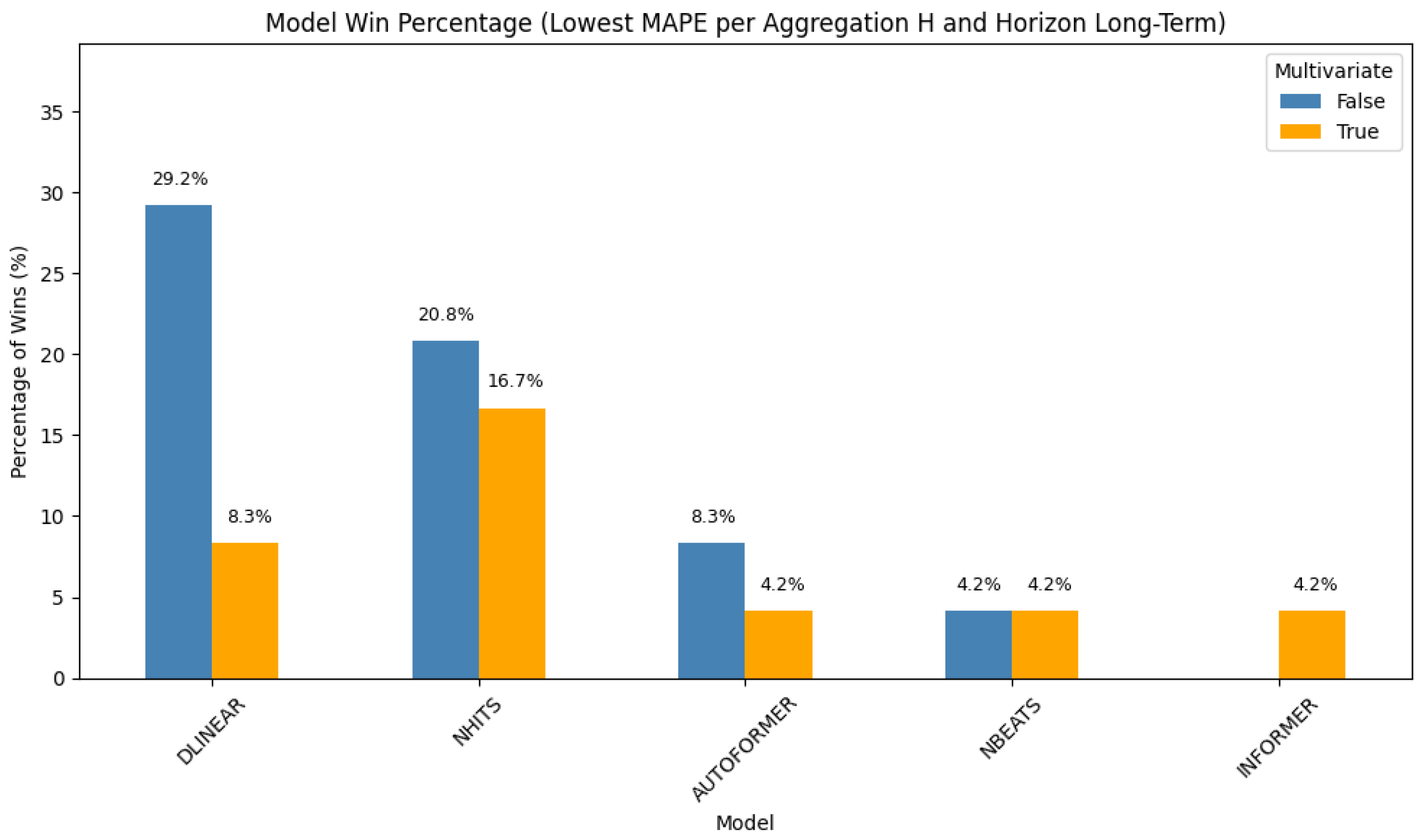
Hourly Aggregation—Long-Term Forecasting

For long-term hourly forecasting (Figure 2), simpler models dominate. Univariate DLinear achieves the highest win rate (29.2%), followed by univariate NHITS at 20.8%. Multivariate NHITS and multivariate DLinear contribute 16.7% and 8.3%, respectively. Additional contributions come from Autoformer, NBEATS, and Informer. These results suggest that, over extended horizons, lightweight models may generalize more effectively due to the reduced risk of overfitting.

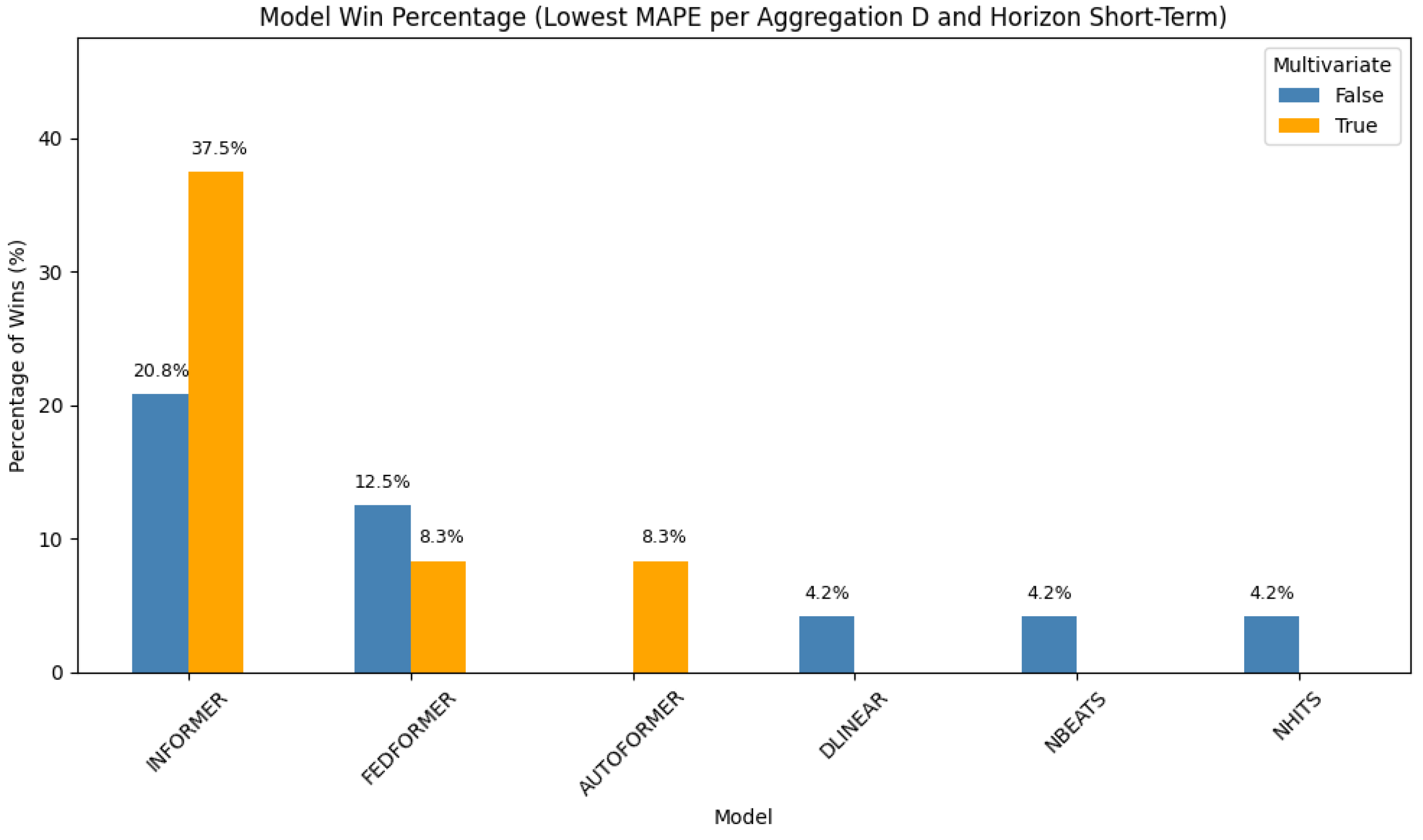
Daily Aggregation—Short-Term Forecasting

Transformer-based models again take the lead in short-term daily forecasting (Figure 3). Multivariate Informer dominates with a 37.5% win rate, followed by its univariate counterpart at 20.8%. FEDformer ranks next, with 12.5% (univariate) and 8.3% (multivariate), respectively. Autoformer contributes 8.3%, and the remaining wins are distributed among DLinear, NBEATS, and NHITS. This highlights the utility of transformers in capturing structured patterns at a daily resolution.

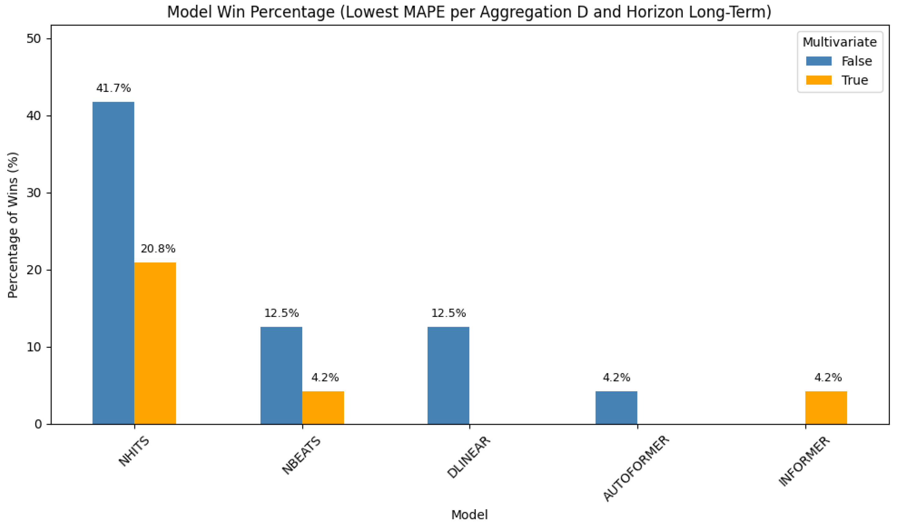
Daily Aggregation—Long-Term Forecasting

In this long-term scenario (Figure 4), simpler models again show superior performance. Univariate NHITS leads with 41.7% of the wins, followed by its multivariate variant at 20.8%. Additional contributions come from NBEATS, DLinear, Autoformer, and FEDformer. These findings reinforce that, for extended daily horizons, architectures with trend decomposition or shallow learning dynamics may be more effective.

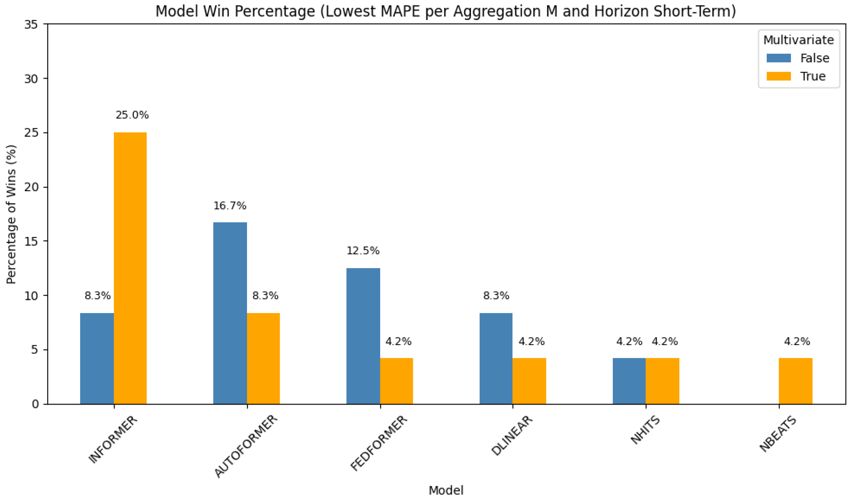
Monthly Aggregation—Short-Term Forecasting

In the short-term monthly setting (Figure 5), transformers once again perform well. Multivariate Informer achieves the highest win rate (25%), followed by univariate Autoformer at 16.7%. Univariate FEDformer, univariate Informer, and multivariate Autoformer each contribute 8.3%. Other performing models include DLinear, NHITS, and NBEATS. These results suggest that transformer models maintain strong performance even in lower-frequency, short-range forecasting.

Monthly Aggregation—Long-Term Forecasting

For long-term monthly predictions (Figure 6), lighter models again prove competitive. Multivariate NBEATS ranks first (20.8%), followed by its univariate form at 16.7%. Informer appears in both forms (12.5% each), while Autoformer and DLinear round out the remaining wins. These outcomes suggest that while transformer models remain competitive, NBEATS in its multivariate form excels in capturing coarse-grained temporal dynamics over longer horizons.

6. Conclusions

In this work, we conducted a comprehensive evaluation of several state-of-the-art deep learning models for time series forecasting, applied to a novel energy–weather dataset spanning 24 European countries. By systematically comparing models across different forecasting horizons, aggregation levels, and input settings (univariate vs. multivariate), we derived both empirical and practical insights that can guide future applications and model selection strategies.

In addition to forecasting accuracy, interpretability and deployment feasibility are essential considerations for real-world applications. Lightweight models such as DLinear and NHITS offer not only competitive performance but also advantages in terms of reduced memory usage and faster training time, making them well-suited for embedded systems and real-time grid operation platforms. Furthermore, models like NBEATS provide a degree of interpretability through their structured decomposition into trend and seasonal components, which can support more informed decision-making by energy providers and system operators.

Although more computationally intensive, transformer-based models such as Informer and FEDformer demonstrated strong performance—particularly in daily forecasting scenarios—and should be considered when predictive accuracy is paramount and resources allow for offline training or cloud deployment. Importantly, all evaluated models are easily accessible through the neuralforecast library, which offers a unified and modular interface. This enables practitioners to efficiently benchmark different architectures under their specific forecasting needs and constraints, supporting reproducible experimentation and practical integration.

Our findings demonstrate that univariate models generally outperform multivariate ones in terms of accuracy, particularly for models like DLinear and NBEATS, which leverage simpler architectures or trend-based decomposition. However, transformer-based architectures such as Informer and FEDformer showed significant gains in multivariate settings, indicating their strength in capturing complex interdependencies between energy demand and weather variables.

From a computational standpoint, DLinear, NBEATS, and NHITS emerged as lightweight and efficient models, making them suitable for deployment in environments with limited resources or real-time constraints. In contrast, transformer-based models such as Autoformer, Informer, and FEDformer demonstrated considerably higher memory usage and training times—factors that must be weighed when scalability and resource efficiency are critical.

Our analysis further revealed that no single model consistently outperforms across all scenarios. Instead, the optimal choice depends on the interplay between forecasting horizon, data granularity, and availability of contextual variables. For instance, Informer led in short-term, high-resolution settings, while NHITS and NBEATS were dominant in long-term forecasting.

In summary, this study highlights the importance of aligning model architecture with task-specific constraints and dataset characteristics. Future work may explore dynamic ensemble approaches, hybrid architectures, or meta-learning frameworks that can adaptively select or combine models based on contextual signals and performance feedback.