FastTree-Guided Genetic Algorithm for Credit Scoring Feature Selection

Abstract

Feature selection is pivotal in enhancing the efficiency of credit scoring predictions, where misclassifications are critical because they can result in financial losses for lenders and exclusion of eligible borrowers. While traditional feature selection methods can improve accuracy and class separation, they often struggle to maintain consistent performance aligned with institutional preferences across datasets of varying size and imbalance. This study introduces a FastTree-Guided Genetic Algorithm (FT-GA) that combines gradient-boosted learning with evolutionary optimization to prioritize class separability and minimize false-risk exposure. In contrast to traditional approaches, FT-GA provides fine-grained search guidance by acknowledging that false positives and false negatives carry disproportionate consequences in high-stakes lending contexts. By embedding domain-specific weighting into its fitness function, FT-GA favors separability over raw accuracy, reflecting practical risk sensitivity in real credit decision settings. Experimental results show that FT-GA achieved similar or higher AUC values ranging from 76% to 92% while reducing the average feature set by 21% when compared with the strongest baseline techniques. It also demonstrated strong performance on small to moderately imbalanced datasets and more resilience on highly imbalanced ones. These findings indicate that FT-GA offers a risk-aware enhancement to automated credit assessment workflows, supporting lower operational risk for financial institutions while showing potential applicability to other high-stakes domains.

1. Introduction

In continued pursuance of economic growth nationwide, financial institutions continue to provide consumer facilities as one of their core business functions. Facilities such as mortgages or personal loans provide borrowers with the necessary funds to purchase various products. Nonetheless, credit scoring plays a pivotal role in deciding whether a loan is to be lent to an applicant, whereby applicants must undergo a rigorous risk assessment process to evaluate their financial stability to approve and lend the facility. Creditworthiness is commonly measured based on the financial factors of the applicants, which include income, credit history, and collateral [1]. From this stance, failing to adhere to the risk assessment process would place any financial institution at risk, especially when loans are expected to default. This underscores that a balanced and low-risk approach is needed to ensure equal opportunities while minimizing financial losses.

For several decades, financial institutions have extensively relied on traditional approaches to assess the eligibility of applicants to approve loans. The approaches varied between judgmental and statistical [2]. Qualitative factors, such as interviewing applicants or judging a business plan by financial experts, are favored in judgmental approaches. The approval of loan applications is subject to the feedback and impressions of these experts, which ultimately vary from person to person. Statistical approaches, on the other hand, utilize quantitative data analysis, based upon which an individual’s eligibility is determined. This includes analysis of the ratios and the use of credit scoring models such as the logit model, linear discriminant analysis, and logistic regression [3]. Both approaches, i.e., statistical and judgmental, were found to be inapt to address the complexity of assessing eligibility and prone to biased decisions. For instance, judgmental approaches rely heavily on human expertise and subjective interpretation, leading to inconsistent decisions and potential bias across credit assessors [4]. Statistical methods tend to reduce this subjectivity, yet they depend on historical behavioral data that is often unavailable for thin-file applicants and often assume linear relationships that rarely capture real-world borrower repayment patterns and evolving feature interactions [5]. Consequently, this exposes institutions to inconsistent and unreliable lending outcomes. These weaknesses motivated the need for data-driven approaches that can generalize informative credit predictors beyond predefined modeling assumptions.

With the advent of machine learning, the prediction of creditworthiness to determine the eligibility of applicants has become possible due to its data-driven prediction process that requires minimal human intervention and domain expertise [6,7,8]. Before that, customers should undergo a rigorous process known as Know Your Customer (KYC), which is required by lending institutions to capture personal and credit history details as part of their official procedures. The information is later loaded into machine learning models for training purposes to generalize their predictions towards new applicants, ultimately supporting decisions for thin file clients. As a result, the adoption of machine learning has seen increased dependence in leading countries, such as the United States, the United Kingdom, and China [9].

A critical step in the Machine Learning (ML) pipeline is feature engineering, which involves identifying influential variables that contribute significantly to the model’s accuracy and ability to distinguish between good customers and defaulters. This process not only ensures better performance but also caters to simplicity and eliminates unnecessary features that have a minimal contribution to the final outcome [10]. In contrast, improperly considering inappropriate or redundant features in the training phase can degrade the model’s ability to provide precise results and worsen its ability to distinguish between classes. Further, the complexity of identifying interdependent relationships requires a thorough mathematical understanding of the problem, particularly linearity and indirect relations among features, which is less rigidly predefined in evolutionary feature selection techniques. These challenges reinforce the need for a feature selection strategy that can explore non-linear interactions, minimize costly misclassifications, and generalize across heterogeneous datasets.

This paper proposes a FastTree-Guided Genetic Algorithm (FT-GA) that embeds FastTree, a gradient-boosting model, to guide the evolutionary search toward more promising regions of the feature space. By incorporating risk-sensitive weighting and separability feedback, FT-GA is designed to maximize predictive accuracy while reducing false-positive and false-negative rates in lending environments. Empirical results demonstrate that FT-GA achieves competitive or superior AUC performance across benchmark credit datasets, particularly under low and moderate imbalance conditions, while reducing feature dimensionality and improving decision separability. The contributions of this paper are summarized as follows:

• The development of a FastTree-Guided Genetic Algorithm (FT-GA) that leverages boosting-based separability feedback to direct evolutionary feature selection toward more informative regions of the search space.
• The demonstration of the effectiveness of evolutionary methods to uniformly address the class imbalance issue across different rates, often requiring pairing the best selection and learning techniques when conventional approaches are considered.
• The introduction of risk-sensitive weighting within the fitness calculation to prioritize class separability over raw accuracy, reflecting the unequal impact of false approvals and false rejections in lending environments.
• Validation of the proposed FT-GA through a comprehensive experimental study using four benchmark credit scoring datasets of varying size and imbalance, showing higher or competitive performance.

The remainder of this paper is structured as follows. Section 2 provides an overview of the topic and focuses on the set of techniques that are effectively used for the selection of characteristics. Section 3 provides the formulation of the problem and highlights the steps involved in generating the results of our proposed method. Finally, the performance of FT-GA is evaluated in Section 4, with traditional and modern feature selection techniques used as a baseline to benchmark our results.

2. Related Work

The field of Artificial Intelligence (AI) has transformed the broader financial ecosystems, including service delivery, customer experience, and market valuation processes. Researchers have explored AI-enabled quality assessment in digital platforms such as crypto wallets [11], reviewed its influence on emerging digital technologies serving financial operations [12], analyzed and eventually supported the integration of data-driven approaches in FinTech service innovation [13]. While these works differ in application focus, they reinforce a shared conclusion that financial decision systems increasingly depend on data-driven modeling and reliable expectations. Thus, this broader transformation underscores the importance of developing robust learning-based frameworks, such as those used in credit scoring, where model performance directly influences risk exposure and institutional outcomes.

As credit scoring is one of the earliest and most regulated applications of AI in finance, it remains a representative case where robustness and risk-alignment are critically tested. In light of that, the quality of feature selection in the ML pipeline is pivotal in determining the effectiveness of credit scoring models, not to mention that real-world credit scoring datasets can be complex and high-dimensional [10]. thus making feature selection a crucial step for financial risk assessment. Over the decades, the shift from judgmental and statistical to ML-based scoring has been driven by the demands for higher predictive accuracy, reduced subjectivity, and the ability to generalize decisions upon thin-file clients [5]. However, as the issue of data complexity and class imbalance continue to grow, fine-grained and adaptable feature selection becomes a cornerstone for constructing robust and generalizable credit scoring models.

This section is intended to review the existing literature that covers four major aspects: the transition from traditional to statistical credit scoring techniques, the adoption of ML in credit scoring, the challenges posed by class imbalance, and the development of feature selection strategies. The objective is to situate this study within existing research and expose gaps in current approaches, particularly limitations in generalizing across datasets, handling imbalance, and over-reliance on accuracy-driven objectives.

2.1. Traditional Credit Scoring

Traditional approaches are crucial to understand to justify the shift towards advanced machine learning models. Banks and lending institutions have relied extensively on judgmental and statistical approaches to assess lending eligibility [2]. The first approach, i.e., judgmental, is intended to assess an applicant’s financial stability in its simplest form. The approach itself relies on qualitative factors, such as interviewing applicants or judging a business plan by financial experts known as “creditors”, and its success is highly dependent on the knowledge and experience of creditors [4,5]. To rectify the dependency on human interpretations, these factors are commonly complemented by systematic and behavioral analyses to apply soft adjustments to judgmental approaches, serving as an essential input when forming credit ratings. These soft adjustments include qualitative disclosure [14], which reflects narrative information that lending firms include in their financial reports, and social network analysis [15] to quantify the ties between individuals to uncover patterns that reflect the repayment behavior of applicants.

Despite that, decisions in judgmental approaches remain subject to the feedback and impressions of creditors, which might vary from person to person. On the other hand, a statistical approach is the practice of relying on statistical models to produce numerical figures determined by relevant data, based on which a decision must be made [5]. Instead, they utilize quantitative data analysis to measure the likelihood that an applicant defaults on a loan. Some known statistical methods include ratio analysis that uses individual financial ratios such as liquidity and profitability, as well as the logit model [3], which builds the model decision based on a probabilistic binary outcome, alongside linear probability [16] and Bayesian models [17].

Both approaches were either biased or highly dependent on historical information recovered from national credit bureaus, with the possibility of the absence of historical credit records, especially in the case of new applicants [2]. The subjectivity issues in judgmental approaches, along with the dependency on historical records in statistical approaches, are two essential factors that declared the need to explore better options to overcome these challenges. In addition, there is no consensus on a universal statistical approach that works under all circumstances, not to mention the time-consuming process of determining which model to use given the situational inputs and the applicability of each method [5].

2.2. Machine Learning in Credit Scoring

High-stakes sectors, including banking and insurance companies, would hesitate to cope with the latest trends. Artificial intelligence (AI) would be no different from any advancements that aim to reshape the financial sector while minimizing apprehensions for its practical adoption. The work of [9] reveals a tremendous expansion of exploration toward the use of ML in the financial sector, particularly in credit scoring. The study highlighted the phenomenal growth in publications since 2021 and stressed the need for more governed ML techniques that account for local regulatory and compliance mandates, while also stressing the need to provide correct results, especially with the susceptibility of ML to provide inaccurate results.

Accuracy in ML has been the ultimate goal sought over the last few years. Hence, tremendous efforts were made to achieve results that are less prone to false positives and true negatives. The work of [7] demonstrated the efficiency of gradient-boosting algorithms in improving prediction accuracy through feature engineering, achieving a precision higher than 93%. Their approach addresses data quality issues, and to overcome this, replacing missing values with averages was an appealing solution, hence underscoring the importance of preprocessing in building reliable models. In particular, better accuracies were achieved when feature selection was incorporated, providing guidance towards more promising search spaces. Similarly, the work of [18] adopted the same strategy, but further elaborated on the adaptability of the models to respond to market shocks. In addition, ref. [8] also managed to determine close accuracies without having to rely on feature engineering, but to make use of multiple models, including Random Forest (RF), Neural Networks (NN) and Linear Discriminant Analysis (LDA) to compare between best performances.

Moreover, traditional ML techniques often fail to capture complex patterns, especially in the case of high-dimensional datasets [19]. This critical issue hinders its practical adoption and potentially degrades the ability of the model to generalize to unseen data. However, real-world datasets are complex and typically have non-linear relationships among features that contribute to the outcome collectively. To address this issue, the authors proposed the Support Vector Machine (SVM) model to solve the high-dimensional and non-linear problem in credit scoring, providing an accuracy of 75% that outperforms that given by RF and Logistic Regression (LR).

Beyond traditional ML models, the work of [20] demonstrated a more advanced, robust, and highly accurate framework that targets small-medium enterprises. The authors introduced the concept of a soft voting multi-staged ensemble model that integrates three advanced ML techniques: LightGBM, XGBoost, and a novel LocalEnsemble module, each utilizing a distinct set of training features to enhance accuracy. The method used adaptive weight optimization to reduce the negative impact of poorly performing models, prioritizing predictions given by better-performing models. The performance of the proposed solution was tested against two real-world credit datasets, namely the Australian and Taiwanese datasets, and demonstrated high accuracy and strong separation capability between classes.

2.3. Class Imbalance in Machine Learning

A common issue across datasets would be the class imbalance, which hinders machine learning models from providing accurate results [10]. This issue is shared across all credit scoring datasets where the number of defaulters is significantly less than that of non-defaulters. This results in significant degradation in generalizing patterns to predict the minority class, suggesting the need for more adaptive techniques that treat all classes equally. On the other hand, this phenomenon implies that class imbalance can potentially lead to failing to provide accurate results when models are tested against actual datasets [8]. Despite excelling in predicting positive cases, models would potentially fail to generalize accurately to minor classes in real-world scenarios.

Many approaches, ranging from data to algorithm levels, have been proposed to overcome the class imbalance issue. However, despite many data sampling techniques have been studied, there is no consensus on the most effective one [21]. This is mainly due to several factors contributing to the effectiveness of each, including the size of the dataset and the imbalance ratio. For instance, the work of [21] compared different undersampling and oversampling techniques to bring classes to equilibrium, denoting that resampling techniques such as Synthetic Minority Over-sampling Technique (SMOT) and Adaptive Synthetic Sampling Approach (ADYSYN) were deemed ineffective when tested against multiple datasets, leading to lower accuracies for some. This is mainly due to their reliance upon oversampling and undersampling of classes, with no prior account for overlapping samples. They also added that these techniques had an insignificant impact on relatively small datasets, while on the contrary, larger datasets exhibiting high-dimensional, complex relations between features and extreme imbalance ratios often led to degraded recall performance, thereby necessitating the careful selection of sampling techniques.

Other studies also considered algorithmic solutions to approach the class imbalance problem. The work presented by [22] demonstrated the effectiveness of the proposed solution to rectify the effect of class imbalance by employing cost-sensitive learning techniques in SVM. Their proposed novel solution efficiently adjusts the separation hyperplane by tuning the error cost of between-class datapoints. Instead of relying on exhaustive grid searches, the solution worked based on balancing between the entropy and the interval to determine the effectiveness of the observed decision boundary and to improve it iteratively.

In addition to cost-tuning, ref. [23] proposed a novel solution that requires assigning competing weights to classes to solve the class imbalance in boost techniques. Unlike sampling and cost-tuning, where the process is time-consuming and computationally expensive, their technique separately determines the best possible setup per class. First, linear programming minimizes each class’s average hinge loss to effectively regulate outliers. Then, a second linear programming is applied to balance between class weights by minimizing the deviation from the class-specific minimum loss determined in the previous step. Despite the general perception that LP can be computationally expensive, the authors also demonstrated that their proposed method is lightweight and efficient, outperforming sampling and cost-sensitive methods in terms of both accuracy and training time in several experimental settings.

2.4. Feature Selection

Feature selection is vital to improve the performance of ML models, and is the process of identifying the most relevant input variables that significantly influence prediction while excluding redundant features [24]. It is deemed useful when a dataset is relatively large, especially when not all features necessarily contribute to the prediction, reducing the dataset’s complexity while ensuring competitive accuracies. The advantage of reduced features extends to reducing the training time needed for ML models.

In filter methods, such as Pearson’s correlation, mutual information, and chi-square tests, the selection of characteristics is determined only based on statistical approaches intended to measure the relationship and contribution of input variables to the predicted output [20]. Pearson correlation is commonly used for linearly defined problems, measuring the magnitude or strength of the linear relationship between one input and the output. For more complex patterns, such as non-linear, mutual information would be a better option due to its capability in capturing the significance of non-linear relationships between the input and output. Lastly, chi-square tests are helpful in evaluating the relationship between categorical inputs against the logistic (binary) outcome. Despite their simplicity, these methods measure the influence of inputs on the output separately, limiting the visibility of selection towards more complex relations and the collective contribution towards the output [25].

In contrast, wrapper methods, such as recursive feature elimination, were designed to account for the collective impact of input variables on the outcome [19]. These methods are intended to measure the interactions between features and output by evaluating different subsets of features. It is achieved by relying on a search strategy that explores the space of possible subsets of features. Many approaches are included in wrapper methods, ranging from forward selection, where the algorithm adds features incrementally and measures the performance gain, to backward elimination, where the algorithm eliminates insignificant features iteratively. Considering that, wrapper methods typically rely on exhaustive searches, which also pose computational concerns, thus limiting their practicality, especially in the case of large datasets [26]. Other metaheuristic optimization techniques, including Particle Swarm Optimization (PSO) [27], Differential Evolution (DE) [28], and Genetic Algorithm (GA) [26], behave as wrapper methods when applied to feature selection, but perform a better guided search, instead of random or exhaustive one.

Another form of feature selection that directly integrates the selection in the training phase is the embedded feature selection. Unlike previous methods, it optimizes feature selection by performing repeated model training based on numerous feature subsets, eventually leading to the best performing subset [29]. Random Forest (RF) is an example of how it generates multiple decision trees to develop predictions and aggregate the results, ultimately improving the accuracy. The steps involved include creating bootstrap samples, forming subsets of data and features, training the decision trees based on the random subsets generated in the previous step, and voting from all the generated trees to predict the classification [30]. A similar approach is given by the Least Absolute Shrinkage and Selection Operator (LASSO), which penalizes the absolute value of coefficients by applying L1 regularization, effectively shrinking some of them to zero, thus excluding them [31].

Although substantial progress has been made in applying different feature selection techniques in the credit scoring domain, ranging from filter-based to wrapper and embedded methods, these methods often fail to generalize well across different datasets having different dimensionalities and class imbalance ratios. Moreover, the applicability of feature selection methods is rarely validated across multiple ML models, raising concerns about their robustness and consistency. To address these limitations, optimization techniques such as the Genetic Algorithm (GA) provide fine-grained searches guided by flexible objective functions. These functions prioritize not only accuracy but also Area Under Curve (AUC), which better reflect class separability as a critical demand in high-stakes environments. By embedding domain-specific priorities into the selection process, the proposed FastTree-guided Genetic Algorithm (FT-GA) aims to identify feature subsets that enhance class distinction and offer a more adaptable and risk-aware solution that generalizes effectively across datasets with varying degrees of imbalance.

3. Proposed Method

The main aim of this study is to propose a hybrid feature selection approach that incorporates FastTrees (Version 3.0.1), a proprietary Microsoft software, to serve as a fitness function to guide the search for GA. The objective of the search is to select the best feature subset that ensures high accuracy while also accounting for data imbalance and separability between classes. FastTrees are a scalable gradient boosting algorithm built on decision trees and is based on the Multiple Additive Regression Trees (MART) algorithm [32]. The FT algorithm itself was initially developed to rank web pages and was then effectively considered for classification and regression tasks. With its ability to optimally handle large and high-dimensional datasets often exceeding memory, FT targets production grade scalability and robustness, often overlooked by traditional algorithms, to better suit real-world datasets [33]. Unlike decision trees that partition data recursively to form a hierarchical structure, the FT algorithm uses an ensemble of shallow decision trees added sequentially to minimize the logistic loss function given in (1). This can be achieved by adopting the stage-wise additive approach in which each successive tree corrects the residuals of the previous ensemble, allowing better generalization and class separation [34].

$$L=\sum _{i=1}^{n}log\left(1+e^{-y_{i}F\left(x_i\right)}\right)$$

(1)

where n is the number of training examples, $y_i\in \{-1,+1\}$ denoting the true label, for example, i, and $F\left(x_i\right)$ is the predicted score. In order to provide the anticipated results of FT-GA, as depicted in Figure 1, let $D=\{(f_i,y_i),i=1,\dots ,n\}$ be the dataset used, where $f_i\in \mathbb{R}$ is used to represent a feature vector corresponding to a particular dataset, and n is the number of instances given in the same dataset. Since the anticipated output is binary denoting the eligibility of applicants, the output $y_i\in \{0,1\}$ would be the class label having only two possible outcomes, i.e., eligible or not. To measure the performance of a given subset, let $c_p=[c_{p1},c_{p2},\dots ,c_{pm}]\in {\{0,1\}}^m$ be the binary chromosome to represent the selection of features given in a dataset, where m is the total number of features present in a particular dataset and generation $p\in \{0,S\}$ to which the chromosome belongs, where S is the total number of iterations and is fixed to a maximum of 50 iterations due to earlier convergence. Typically, a chromosome vector $c_p$ represents a subset of features $f_i$. Therefore, the selected feature set for chromosome $c_p$ is given by (2).

$$F_c=\left\{f_i\left[{\mathbf{c}}_{\mathbf{p}}\right]|i=1,\dots ,n;p\in \{0,S\}\right\}$$

(2)

where $f_i\left[c\right]$ is the result of applying a chromosome mask $c_p$ to each instance $f_i$ to retain the selected features. Each of these chromosomes is used to train the FT classifier and validated using a 30–70% split to generate the accuracy and AUC. Although the 30–70% split enables rapid fitness evaluation inside the evolutionary loop, it constitutes only the internal scoring mechanism of FT-GA. To ensure that reported performance is statistically reliable and not dependent on a single train–test partition, final results for FT-GA and all baselines were additionally evaluated under 10-fold stratified cross-validation. This decouples the optimization speed from generalization validity by assessing stability estimates through mean performance and variance measures later on. Considering the trade-off nature between accuracy and the model’s ability to separate between classes, particularly in binary classification problems [35], two static weights $\alpha$ and $\beta$ are multiplied by accuracy and AUC respectively to represent the balance between the two, as shown in (3) to determine the fitness of $F_c$. It is worth noting that the values assigned to these two static weights reflect the domain-specific risk preference.

$$\mathrm{Fitness}\left(c_p\right)=\alpha \times \mathrm{Accuracy}\left(F_c\right)+\beta \times \mathrm{AUC}\left(F_c\right);\alpha ,\beta \in [0,1],\alpha +\beta =1$$

(3)

where the values of $\alpha$ and $\beta$, and are subject to domain specifications and risk tolerance levels to reflect risk tolerance. In this work, we grounded our decision on the principle of Hofmann stated in the data set [36]: “It is worse to class a customer as good when they are bad, than it is to class a customer as bad when they are good.”, therefore emphasizing AUC to minimize false positives, which is more risky in credit assessment. In light of that, weights of 20% and 80% have been assigned to the accuracy and AUC respectively to favor class separation over opportunity capture, acknowledging that false positives pose greater financial risk than false negatives, thereby making our approach particularly well-suited for conservative financial environments. This decision is supported by previous studies, such as the work given by [37], which explicitly highlight the importance of prioritizing AUC over other metrics to achieve better separability between classes. The Algorithm 1 shows the steps involved in convergent to solutions that prioritize class separation over precision.

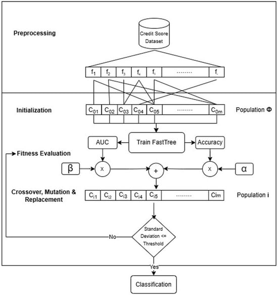
Figure 1. Proposed method resembling FT-GA.

To ensure proper hyper parametrization of our proposed method, various GA configuration parameters have been considered in this work to encourage better feature subset exploration. The population size included 10, 30, and 50 chromosomes to account for computational costs and convergence speed. Furthermore, two crossover points have been considered with crossover rates ($r_c$) varying between 0.6 and 0.8, as well as gene and chromosome mutation techniques with 0.05 probability rate of mutation rate ($r_m$) in order to introduce diversity into a single population. The selection of parent chromosomes to produce offspring was based on tournament and roulette-wheel selections, with tournament sizes varying between 2 and 5. To retain quality solutions, a rate of 0.1 was assigned to ($r_e$) to preserve 10% of the elite chromosomes. Lastly, all attempts to measure the sensitivity of GA configuration parameters were executed for 50 iterations to observe the convergence speed across populations. To tune these parameters, each parameter value was perturbed independently while holding others constant, enabling observation of marginal performance shifts on AUC and accuracy under the fitness weighting considered. This resulted in 36 configurations, from which settings were selected that consistently balanced between accuracy and separability improvements while avoiding excessive runtime or premature convergence. Table 1 shows the set of GA configuration parameters used for each dataset, chosen for their suitability after conducting a parameter sensitivity analysis.

Algorithm 1: Feature Selection with FastTree

Table 1. Parameter Configuration for FT-GA.

Dataset	GA Configuration
Australian	Population size (30), Single-point (rc = 0.8), gene mutation (rm = 0.05), Tournament size (5)
German	Population size (50), Single-point (rc = 0.8), gene mutation (rm = 0.05), Tournament size (3)
Japanese	Population size (30), Single-point (rc = 0.8), gene mutation (rm = 0.05), Tournament size (3)
Taiwanese	Population size (30), Single-point (rc = 0.6), gene mutation (rm = 0.05), Tournament size (3)

3.1. Datasets Description & Preprocessing

To evaluate the performance of our proposed solution, four real-world credit score datasets retrieved from UCI and Kaggle have been selected to assess various metrics, including the size of the dataset, the number of features included in the final subset, class imbalance, and generalizability of the FT-GA. The datasets included in our experiment were German credit data [36], Australian credit approval [38], Japanese credit scoring [39], and Taiwanese default of credit card clients [40]. The variety of datasets is intended to promote generalizability and credibility among diverse borrower populations. These datasets were intentionally selected because they are widely used benchmarks in credit scoring research, publicly available, and vary in size and imbalance ratios, allowing FT-GA to be evaluated across realistic operational conditions. Moreover, each dataset contains the core risk factors traditionally used in lending decisions, i.e., demographics and repayment history, meaning their indicators align with theoretical and regulatory practice in credit risk modeling.

The number of instances included varied between datasets, with the Australian dataset having 690 instances at a minimum and more than 30,000 instances given in the Taiwanese dataset at a maximum. This allows our method to be evaluated across small, medium, and large-scale scenarios to assess its scalability. Moreover, all selected datasets were meant to provide varying ratios of class imbalance, with the Taiwanese dataset scoring the highest imbalance ratio, and the Japanese and Australian datasets having balanced datasets. Table 2 shows the distribution of percentages among defaults and non-defaults for the four datasets.

Table 2. Distribution of Classes per Dataset.

Dataset	True Class (%)	False Class (%)
Australian	44.49	55.51
German	70.00	30.00
Japanese	44.49	55.51
Taiwanese	22.12	77.88

The number of features included within each dataset varied significantly, and only a slight preprocessing has been applied to each, which include:

• Label encoding of categorical features given in the German credit score dataset.
• Handling mixed data types, mostly strings and numbers, given in the Australian credit approval dataset. Label encoding was applied to non-numeric features to ensure that the models could process them.
• Replace missing categorical values with the mode and averaging continuous values in the Japanese dataset before encoding them, and converting the target variable labels to binary in order to be consistent with other datasets.

Both German and Taiwanese datasets explicitly provide feature names, while features included in Japanese and Australian datasets were anonymized for privacy purposes. Table 3 and Table 4 show all attributes included in the German and Taiwanese datasets with their data types, respectively.

Table 3. Attributes of the German Credit Score Dataset.

No.	Attribute	Data Type
1	Status of Existing Checking Account	String
2	Duration (Month)	Numeric
3	Credit History	String
4	Purpose	String
5	Credit Amount	Numeric
6	Savings Account/Bonds	String
7	Present Employment Since	String
8	Installment Rate In Percentage of Disposable Income	Numeric
9	Sex	String
10	Personal Status	String
11	Other Debtors Guarantors	String
12	Present Residence Since	Numeric
13	Property	String
14	Age (Years)	Numeric
15	Other Installment Plans	String
16	Housing	String
17	Number of Existing Credits at This Bank	Numeric
18	Job	String
19	Number of People Being Liable to Provide Maintenance For	Numeric
20	Telephone	String
21	Foreign Worker	String

Table 4. Attributes of the Taiwanese Credit Card Defaults Dataset.

No.	Attribute	Data Type
1	LIMIT_BAL	Numeric
2	SEX	Numeric
3	EDUCATION	Numeric
4	MARRIAGE	Numeric
5	AGE	Numeric
6	PAY_0	Numeric
7	PAY_2	Numeric
8	PAY_3	Numeric
9	PAY_4	Numeric
10	PAY_5	Numeric
11	PAY_6	Numeric
12	BILL_AMT1	Numeric
13	BILL_AMT2	Numeric
14	BILL_AMT3	Numeric
15	BILL_AMT4	Numeric
16	BILL_AMT5	Numeric
17	BILL_AMT6	Numeric
18	PAY_AMT1	Numeric
19	PAY_AMT2	Numeric
20	PAY_AMT3	Numeric
21	PAY_AMT4	Numeric
22	PAY_AMT5	Numeric
23	PAY_AMT6	Numeric

3.2. Baseline ML Models

To assess the performance of FT-GA, a set of feature selection techniques has been considered to train a set of well-known ML models. The results given by each pair, i.e., selection technique to train the ML model, will serve as a baseline to benchmark the results of our proposed method. Traditional and modern feature selection techniques highlighted in the literature were used to select a subset of features to train the following ML models.

1.

Logistic Regression (LR): a simple statistical model considered to be a special type of linear regression formula being substituted in the logistic (sigmoid) function [6]. It aims to optimally determine the values of the coefficients ($\beta$) given in the linear formula, thereby predicting the output for a given set of inputs. The formula for a logistic regression is as shown in (1).

$$\sigma ={\displaystyle \frac{1}{1+e^{-y}}};y=\left[\sum _{i=0}^n{\beta }_i{X}_i\right]+\epsilon$$

(4)

where ${\beta }_i$ is the optimized coefficient for the data point $X_i$, and the value of $\sigma$ determines the probability $[0\dots 0.5\dots 1]$ to classify datapoints. LR is mostly efficient for solving linear problems only.

2.

Naïve Bayes (NB): a supervised machine learning model that operates based on the Bayes theorem. This model operates under the assumption that the input features are conditionally independent given a predicted class [41]. It is particularly efficient for classification problems where this independence assumption approximately holds true despite its simplicity. By multiplying the probability of evidence if the outcome is true $\left(P(X\mid y)\right)$ by how common that outcome is $\left(P\left(y\right)\right)$, and dividing by how common the evidence (observations) is overall $P\left(X\right)$, the probability of a given result is determined given the observed evidence $\left(P(y\mid X)\right)$, as shown in (2).

$$P(y\mid X)={\displaystyle \frac{P(X\mid y)·P\left(y\right)}{P\left(X\right)}}$$

(5)

3.

Random Forest (RF): An ensemble learning model that produces multiple decision trees to formulate its prediction. The algorithm works by constructing a ‘forest’ of Decision Trees (DTs) to aggregate the results, thereby improving its accuracy. It resolves the issue of overfitting by relying on identically distributed decision trees to reach a majority vote. The steps involved include creating bootstrap samples, forming subsets of data and features, training the decision trees based on the random subsets generated in the previous step, and predicting the classification based on votes given by all generated trees [30]. The core concept of RF lies in minimizing the Gini impurity that measures the probability of incorrectly classifying a randomly chosen sample, as shown in (3).

$$Gini\left(D\right)=1-\sum _{k=1}^n{P}_n^2,P_n={\displaystyle \frac{\mathrm{Samples}\mathrm{in}\mathrm{class}\left(n\right)}{\mathrm{Total}\mathrm{samples}\mathrm{in}\mathrm{node}}}$$

(6)

4.

Artificial Neural Networks (ANN): inspired by how the human brain works, and comprises several neural nodes receiving an input, processing it, and producing an output signaled to the subsequent node. It consists of three main layers: the input layer receiving inputs, the hidden layer comprising one or more nodes, and adjusts the weights and biases to capture hidden patterns, as well as the output layer which provides the classification [42] based on a chosen transfer function. Our baseline considers only feed-forward NN with Sigmoid transfer to provide the logistic prediction.

3.3. Performance Metrics & Evaluation

Since the problem presented in this research is modeled as a binary classification problem, a set of well-known performance metrics, including accuracy, AUC, recall, and precision [43] have been adopted to assess the performance of our proposed method along with the baseline solutions. For each best-performing pair comprising the feature selection method used and the ML model to provide the prediction, all metrics highlighted in Equations (7)–(10) have been used to determine the suitability of our method. To achieve a lower risk approach, the AUC metric was prioritized over other metrics that concern positive classes, including precision and recall. The AUC will determine the effectiveness of our proposed method in separating class labels, and its value can be between 0 and 1 whereby an efficient classifier would have an AUC value close to 1 [44].

$$\mathrm{Accuracy}={\displaystyle \frac{TP}{TP+TN+FP+FN}}$$

(7)

$$\mathrm{Recall}={\displaystyle \frac{TP}{TP+FN}}$$

(8)

$$\mathrm{Precision}={\displaystyle \frac{TP}{TP+FP}}$$

(9)

$$F1-\mathrm{Score}=2\times {\displaystyle \frac{\mathrm{Precision}\times \mathrm{Recall}}{\mathrm{Precision}+\mathrm{Recall}}}$$

(10)

• True Positive (TP): the classifier predicted that an applicant is eligible, in which they are in reality eligible. Therefore, it Measures the classifier’s capability to capture actual positive cases.
• False Positive (FP): the classifier incorrectly predicts an applicant to be eligible when they are in reality not. From the perspective of a lending institution, this could potentially lead to a financial loss due to a possible default.
• True Negative (TN): the classifier correctly predicts that an applicant is not eligible, in which in reality they are not. It measures the classifiers capability to correctly capture actual negative cases corresponding to non-eligible applicants.
• False Negative (FN): the classifier incorrectly predicts that an applicant is not eligible, when they actually are eligible. From the perspective of a lending institution, this forms a potential opportunity loss.

To compare performance between all pairs, in addition to accuracy and AUC, other key performance metrics such as recall, precision, and f1 score have also been considered to reflect overall performance. Equations (7)–(10) provide the formulas used to determine all metrics based on the results given in the confusion matrix. For FT-GA and all baseline models, performance reporting follows 10-fold stratified cross-validation rather than a single split, in order to mitigate sampling variability and ensure statistical robustness. For each best performing pair, mean values and standard deviations were computed for accuracy and AUC, alongside Kolmogorov–Smirnov (KS) distance as a separability indicator to strengthen the comparability by evaluating stability across folds rather than isolated test outcomes.

4. Results & Discussion

This work aims to provide a low-risk approach to balance the trade-off between accuracy and separation between classes. The results of the experiment were generated in two phases: First, the selection of features was made using different feature selection techniques highlighted previously, including Chi2-square (Chi2), Mutual Information (MI), Recursive Feature Elimination (RFE), Logistic Regression with L1 regularization (L1 LogReg), and Random Forest (RF). Then, each subset given by the feature selection technique is used to train four different ML models, including Logistic Regression (LR), Naïve Bayes (NB), Random Forest (RF), and Neural Network (NN). The results of all pairs are later used to compare and benchmark those given by FT-GA. For simplicity, the best-performing pairs have been considered to ensure that our proposed solution is in line with the best possible configurations. Table 5, Table 6, Table 7 and Table 8 show the feature subsets determined by different methods corresponding to each dataset. Notably, FT-GA tends to converge on compact subsets that do not focus on reducing dimensions butrather preserve domain-meaningful weighting between accuracy and AUC. It suggests that its separability-driven objective sought by GA implicitly favors features relevant to risk signaling rather than generic feature reduction or accuracy-focused techniques. This observation is evidenced by the varying number of features maintained across the four distinct datasets and suggests that FT-GA adapts to different datasets rather than applying a uniform feature importance pattern, thereby reinforcing its suitability for heterogeneous credit scoring contexts.

Table 5. Feature Subsets Determined By Different Methods for the Australian Credit Dataset.

Selection Method	Selected Features
Chi2	A2, A3, A5, A6, A7, A8, A9, A10, A13, A14
MI	A4, A5, A6, A7, A8, A9, A10, A12, A13, A14
RFE	A1, A4, A5, A6, A7, A8, A9, A10, A11, A12
L1_LogReg	A1 to A14
RF	A2, A3, A5, A7, A8, A10, A14
FT-GA	A1, A2, A3, A6, A7, A8, A9, A10, A11, A12, A13, A14

Table 6. Feature Subsets Determined By Different Methods for the Japanese Credit Dataset.

Selection Method	Selected Features
Chi2	A2, A3, A5, A6, A8, A9, A10, A11, A14, A15
MI	A4, A5, A6, A7, A8, A9, A10, A11, A14, A15
RFE	A1, A4, A5, A6, A7, A8, A9, A10, A11, A12
L1_LogReg	A1, A2, A3, A4, A5, A6, A7, A8, A9, A10, A11, A12, A13, A14, A15
RF	A2, A3, A8, A9, A10, A11, A14, A15
FT-GA	A3, A5, A6, A9, A11, A13, A15

Table 7. Feature Subsets Determined By Different Methods for the Taiwanese Credit Dataset.

Selection Method	Selected Features
Chi2	LIMIT_BAL, PAY_2, PAY_3, BILL_AMT1, BILL_AMT2, BILL_AMT3, BILL_AMT4, BILL_AMT5, BILL_AMT6, PAY_AMT1
MI	LIMIT_BAL, PAY_0, PAY_2, PAY_3, BILL_AMT1, BILL_AMT2, BILL_AMT3, PAY_AMT1, PAY_AMT2, PAY_AMT3
RFE	LIMIT_BAL, SEX, EDUCATION, MARRIAGE, PAY_0, PAY_2, BILL_AMT1, BILL_AMT3, PAY_AMT1, PAY_AMT2
L1_LogReg	LIMIT_BAL, SEX, EDUCATION, MARRIAGE, AGE, PAY_0, PAY_2, PAY_3, PAY_4, PAY_5, PAY_6, BILL_AMT1, BILL_AMT2, BILL_AMT3, BILL_AMT4, BILL_AMT5, BILL_AMT6, PAY_AMT1, PAY_AMT2, PAY_AMT3, PAY_AMT4, PAY_AMT5, PAY_AMT6
RF	LIMIT_BAL, PAY_0, PAY_2, BILL_AMT1, BILL_AMT2, BILL_AMT3, PAY_AMT1, PAY_AMT2, PAY_AMT3, PAY_AMT6
FT-GA	LIMIT_BAL, SEX, EDUCATION, PAY_0, PAY_3, PAY_4, PAY_5, PAY_6, BILL_AMT1, BILL_AMT2, BILL_AMT6, PAY_AMT2

Table 8. Feature Subsets Determined By Different Methods for the German Credit Dataset.

Selection Method	Selected Features
Chi2	Status of Existing Checking Account, Duration (Month), Credit History, Purpose, Credit Amount, Savings Account/Bonds, Present Employment Since, Installment Rate In Percentage of Disposable Income, Personal Status, Age (Years)
MI	Status of Existing Checking Account, Duration (Month), Credit History, Purpose, Credit Amount, Savings Account/Bonds, Sex, Other Debtors/Guarantors, Present Residence Since, Foreign Worker
RFE	Status of Existing Checking Account, Credit History, Savings Account/Bonds, Present Employment Since, Installment Rate In Percentage of Disposable Income, Personal Status, Other Installment Plans, Job, Number of People Being Liable to Provide Maintenance For, Foreign Worker
L1 LogReg	Status of Existing Checking Account, Duration (Month), Credit History, Purpose, Credit Amount, Savings Account/Bonds, Present Employment Since, Installment Rate In Percentage of Disposable Income, Sex, Personal Status, Other Debtors/Guarantors, Present Residence Since, Property, Age (Years), Other Installment Plans, Housing, Number of Existing Credits At This Bank, Job, Number of People Being Liable to Provide Maintenance For, Telephone, Foreign Worker
RF	Status of Existing Checking Account, Duration (Month), Credit History, Purpose, Credit Amount, Savings Account/Bonds, Present Employment Since, Installment Rate In Percentage of Disposable Income, Present Residence Since, Property, Age (Years)
FT-GA	Status of Existing Checking Account, Duration (Month), Present Employment Since, Installment Rate In Percentage of Disposable Income, Sex, Other Debtors/Guarantors, Property, Age (Years), Other Installment Plans, Number of Existing Credits At This Bank, Job, Number of People Being Liable to Provide Maintenance For, Telephone

Table 9 provides the overall performance between the best-performing pairs retrieved from Table A1, Table A2, Table A3 and Table A4 listed in the Appendix A, and Figure 2a–d visualize their AUC in all datasets used. Overall, FT-GA demonstrated competitive results, especially with those given by RF, and better adaptability across different datasets. This is evidenced by the numerous combinations pairing feature selection and training models in order to achieve close results, considering the inclusion of top-performing baselines only. This positions FT-GA as a robust and generalizable choice to balance between feature reduction and obtaining contextual results, which in our case include accuracy and separability between classes. The same applies from a risk-assessment standpoint, where our proposed method achieved the highest AUC values for relatively smaller datasets, in the case of Australian and Japanese datasets, and also maintained a good balance between offering opportunities to applicants and flagging potential defaulters. This balance was demonstrated by recall values exceeding 0.90 and 0.88 for the Australian and Japanese datasets, respectively. It is also worth noting that variation in model accuracy across datasets is expected, as performance is inherently influenced by dataset complexity, particularly differences in sample size and class imbalance. Accordingly, datasets with milder imbalance and clearer signal structure yielded higher predictive ceilings, whereas highly imbalanced or larger ones imposed lower attainable accuracy levels for all competing methods. Nonetheless, the results suggest that FT-GA performs best when minority class representation is sufficient for the boosting component to learn discrimination boundaries, whereas traditional methods tend to overfit majority behavior. In general, this reflected a higher level of flexibility in terms of guiding a selection method towards more promising and domain-specific results, thereby aligning with practical needs.

Table 9. Overall performance between the best-performing pairs.

Dataset	Method	Features	Accuracy	Precision	Recall	F1 Score	AUC
Australian	Chi-LR	10	0.8599	0.8819	0.8889	0.8854	0.9217
	MI-RF	10	0.8647	0.8889	0.8889	0.8889	0.9254
	RFE-RF	10	0.8744	0.8846	0.9127	0.8984	0.9209
	L1-RF	14	0.8696	0.8898	0.8968	0.8933	0.9291
	RF-RF	7	0.8744	0.9032	0.8889	0.8960	0.9253
	FT-GA	12	0.8760	0.8830	0.9022	0.8925	0.9287
German	Chi-NB	10	0.7400	0.7631	0.9091	0.8297	0.7683
	MI-LR	10	0.7267	0.7471	0.9187	0.8240	0.7773
	RFE-NB	10	0.6967	0.8554	0.6794	0.7573	0.7979
	L1-NB	21	0.7467	0.8093	0.8325	0.8208	0.7830
	RF-RF	11	0.7600	0.7773	0.9187	0.8421	0.7662
	FT-GA	13	0.8480	0.8862	0.9321	0.9086	0.8543
Japanese	Chi-RF	10	0.8599	0.8542	0.8454	0.8497	0.9202
	MI-RF	10	0.8261	0.8081	0.8247	0.8163	0.9146
	RFE-LR	10	0.8406	0.7909	0.8969	0.8406	0.9054
	L1-LR	15	0.8309	0.7870	0.8763	0.8293	0.8973
	RF-RF	8	0.8551	0.8317	0.8660	0.8485	0.9065
	FT-GA	7	0.8554	0.8077	0.8832	0.8438	0.9223
Taiwanese	Chi-RF	10	0.7847	0.5129	0.2230	0.3108	0.6971
	MI-RF	10	0.8014	0.5713	0.3536	0.4368	0.7337
	RFE-RF	10	0.7873	0.5271	0.2281	0.3184	0.6985
	L1-RF	23	0.8133	0.6230	0.3617	0.4577	0.7549
	RF-RF	10	0.8131	0.6287	0.3464	0.4467	0.7406
	FT-GA	12	0.8116	0.6369	0.3570	0.4575	0.7680

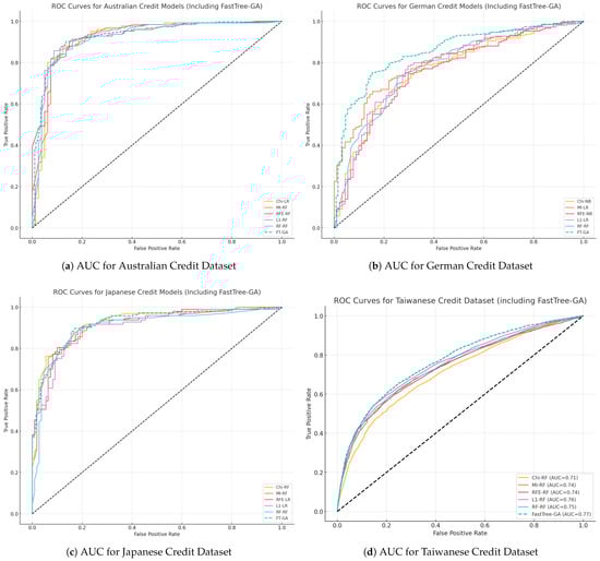
Figure 2. AUC for all solutions visualized by dataset: (a) Australian, (b) German, (c) Japanese, (d) Taiwanese.

Across all datasets, the AUC for FT-GA shown in Figure 2a–d consistently resembled superior or similar separation capability between the two classes with reference to the baseline pairs, confirming its ability to minimize false positive results. In addition, FT-GA demonstrated its capability to handle imbalanced data in smaller datasets, particularly in the German dataset, where the data were moderately imbalanced. The AUC given in Figure 2b serves as a proof that FT-GA provides better separation between the two classes, thereby ensuring less risky decisions. Moreover, the performance of FT-GA on the German dataset also accounted for providing the best results in terms of accuracy, precision, and recall, with values of 0.84, 0.88, 0.93 respectively. This concludes that FT-GA managed to distinguish between defaulters and non-defaulters, while also accounting for fair opportunities to eligible applicants with no compromise. These findings emphasize the stability and generalization of FT-GA across moderately imbalanced datasets that are small in size. Interestingly, FT-GA achieved higher recall without requiring aggressive resampling, a common preprocessing requirement for imbalanced datasets, implying that the separability weighting in its objective function compensates for imbalance by rewarding clearer minority class splits.

To further validate robustness beyond single train–test performance, a 10-fold cross-validation experiment was conducted across all datasets, and the aggregated results are reported in Table 10. These results provide additional evidence of the stability of FT-GA relative to competing feature selection–model pairs. Notably, FT-GA achieved the highest AUC and KS statistics in the German and Taiwanese datasets, while maintaining competitive performance in the Australian and Japanese cases despite slightly lower mean accuracy. The relatively lower standard deviation in AUC observed for FT-GA across folds, particularly in the German dataset, supports its generalization capacity, indicating that the prioritized separability objective yields more stable class boundary learning than accuracy-based approaches. These outcomes reinforce the earlier observation that FT-GA performs more effectively where minority class representation and imbalance conditions provide meaningful discrimination cues.

Table 10. 10-fold cross-validation results across all datasets.

Dataset	Pair	ACC (Mean)	AUC (Mean)	AUC (std)	KS (Mean)
Australian	Chi–LR	0.8710	0.9144	0.0380	0.7817
	MI–RF	0.8594	0.9102	0.0429	0.7823
	RFE–RF	0.8623	0.9083	0.0500	0.7710
	L1–RF	0.8596	0.9155	0.0384	0.7607
	RF–RF	0.8580	0.9115	0.0411	0.7530
	FT–GA	0.8562	0.9145	0.0364	0.7549
German	Chi–NB	0.7250	0.7526	0.0419	0.4724
	MI–LR	0.7540	0.7810	0.0398	0.4838
	RFE–NB	0.6740	0.7241	0.0517	0.4224
	L1–NB	0.7130	0.7498	0.0516	0.4852
	RF–RF	0.7700	0.7785	0.0359	0.4833
	FT–GA	0.8194	0.8447	0.0268	0.6309
Japanese	Chi–RF	0.8638	0.9361	0.0528	0.7683
	MI–RF	0.8638	0.9283	0.0461	0.7873
	RFE–LR	0.8565	0.9231	0.0569	0.7860
	L1–LR	0.8667	0.9330	0.0494	0.7604
	RF–RF	0.8621	0.9311	0.0541	0.7671
	FT–GA	0.8532	0.9200	0.0288	0.7666
Taiwanese	Chi–RF	0.7928	0.7098	0.0070	0.3215
	MI–RF	0.8066	0.7418	0.0052	0.3771
	RFE–RF	0.8080	0.7411	0.0069	0.3796
	L1–RF	0.8135	0.7579	0.0047	0.3991
	RF–RF	0.8103	0.7445	0.0077	0.3796
	FT–GA	0.8185	0.7767	0.0129	0.4231

Despite the compelling results, however, all techniques fell short to handle extreme data imbalances, and it worht noting that the true strength of FT-GA lies in handling small to medium-sized datasets with moderate imbalance ratios. Moreover, in cases of extreme data imbalance, such as the case of Taiwanese dataset, the proposed solution still outperformed baseline methods not exclusively in AUC, but also in all other metrics, including accuracy, precision, and recall, as evidenced in the German and Taiwanese dataset results. However, despite that FT-GA comparably showed slightly better resilience and delivered the best results across all performance metrics, the results suggest that integrating sampling techniques in the preprocessing phases could further enhance the process and abolish the effect of larger imbalance ratios. Thus, it signifies an opportunity to extend our current method with hybrid strategies to make it more resilient in a broader range of imbalance scenarios, and suggests that while FT-GA is still resilient, its risk-guided objective function relies on a minimum signal from the minority class when imbalance becomes extreme, therefore the boosting guidance weakens.

In addition, the comparative results show that FT-GA achieves performance that is broadly comparable to state-of-the-art solutions, despite fundamentally addressing the feature selection scope of the scoring pipeline, as shown in Table 11. In cases where FT-GA trails deep learning or boosting methods, such as gcForest and AugBoost-ELM, the accuracy gap remains below 4%, which is consistent with expectations given that these methods learn internal feature representations rather than selecting transparent subsets as in our approach. More importantly, FT-GA delivers similar or better AUC performance across multiple studies, aligning with its objective of maximizing class separability rather than maximizing raw accuracy. Unlike pipeline-based or ensemble models that incorporate sampling, stacking, multi-layer transformations, or meta-parameter tuning, FT-GA is a single-stage optimization mechanism that neither resamples nor augments representations and yet attains comparable predictive capability.

Table 11. Comparison between published results and FT-GA expressed in delta performance.

Study	Dataset	Model	ACC (%)	AUC (%)	$\mathbf{\Delta }$ACC	$\mathbf{\Delta }$AUC
Zhang et al. (2018) [30]	Australian	NCSM (Deep Learning)	91.71	–	−4.11	–
	German	NCSM (Deep Learning)	82.14	–	+2.66	–
Yao & Chen (2019) [45]	German	SVM-RF (Hybrid Ensemble)	83.55	84.00	+1.25	+1.43
	Australian	SVM-RF (Hybrid Ensemble)	87.94	92.10	−0.34	+0.77
Dumitrescu et al. (2022) [6]	Australian	PLTR (Hybrid)	–	92.99	–	−0.12
Goh et al. (2020) [46]	German	SVM-RF (Hybrid)	76.40	80.44	+8.40	+4.99
	Australian	SVM-RF (Hybrid)	87.38	86.14	+0.22	+6.73
Li et al. (2021) [47]	German	gcForest (Two-stage Hybrid Deep Forest)	81.20	86.80	+3.60	−1.37
	Australian	gcForest (Two-stage Hybrid Deep Forest)	88.55	94.25	−0.95	−1.38
	Japanese	gcForest (Two-stage Hybrid Deep Forest)	88.99	96.02	−3.45	−3.79
Zhang et al. (2021) [48]	Taiwanese	Hybrid Ensemble	80.50	79.37	+0.66	−2.57
Bao et al. (2019) [49]	German	Supervised + Unsupervised Hybrid	80.80	–	+4.00	–
Yuan et al. (2022) [50]	Australian	K-means + SVDD	–	84.86	–	+8.01
	German	K-means + SVDD	–	65.71	–	+19.72
	Japanese	K-means + SVDD	–	85.17	–	+9.12
Jin et al. (2021) [51]	Australian	Multi-stage Ensemble + K-Means	–	93.98	–	−1.11
	German	Multi-stage Ensemble + K-Means	–	77.96	–	+7.47
	Japanese	Multi-stage Ensemble + K-Means	–	92.48	–	−0.25
Jiao et al. (2021) [52]	Australian	APSO-XGBoost	88.20	–	−0.60	–
	German	APSO-XGBoost	77.48	–	+7.32	–
Rofik et al. (2024) [53]	German	Stacking Ensemble	83.21	–	+1.59	–
Liu et al. (2021) [54]	Australian	mg-mGBDT	88.26	94.07	−0.66	−1.20
	Taiwanese	mg-mGBDT	69.22	75.16	+11.94	+1.64
	Japanese	mg-mGBDT	86.90	93.11	−1.36	−0.88
	German	mg-mGBDT	76.53	78.46	+8.27	+6.97
Zou & Gao (2022) [55]	Australian	AugBoost-ELM	86.35	94.22	−1.55	−1.35
	German	AugBoost-ELM	76.17	78.61	+8.63	+6.82
	Japanese	AugBoost-ELM	86.87	93.99	−1.33	−1.76
	Taiwanese	AugBoost-ELM	69.63	75.16	+11.53	+1.64
Yotsawat et al. (2021) [56]	German	XGB-BO	79.50	80.50	+5.30	+4.93
	Australian	XGB-BO	88.70	93.25	−3.90	−0.38

When relating FT-GA to prior studies, three performance patterns emerge. First, on the German dataset, which reflects moderate imbalance and resembles realistic credit risk distributions, FT-GA consistently outperformed many sophisticated architectures, including hybrid ensembles and deep-learning–inspired designs, across both accuracy and AUC. The only exception was gcForest, where FT-GA fell behind marginally by −1.37% in terms of AUC, a gap attributable to gcForest’s hierarchical multi-layer forest structure that learns latent representations far beyond what conventional feature selectors are intended to capture. Second, FT-GA demonstrated substantial separability advantages relative to traditional and clustering-based approaches such as K-means + SVDD, where AUC gains exceeded 19 percentage points, and remained favorable even against SVM–RF hybrids (+0.77% AUC). Conversely, FT-GA’s largest performance deficits occurred on small balanced datasets such as Australian and Japanese credit scoring, with gcForest again exhibiting the largest advantage (−3.79% AUC). These behaviors reinforce that FT-GA is better aligned with operational scenarios characterized by moderate imbalance and meaningful minority representation, whereas deep/hybrid pipelines gain modeling capacity on compact datasets through representational learning.

Third, a similar behavior was observed in accuracy comparisons, where FT-GA outperformed most published methods, often by up to 12%, however trailed slightly when compared with more sophisticated boosting and deep learning architectures. This slight deficit, however, must be interpreted in light of methodological scope; FT-GA is a simple, purely evolutionary feature selector requiring no representation learning, resampling, stacked architectures, or deep composition layers. Unlike gcForest and hybrid ensembles, FT-GA performs no internal augmentation or multi-stage inference, yet its performance gaps remain consistently small, and typically between 2–4%. This suggests that FT-GA offers a favorable accuracy–efficiency trade-off, achieving competitive risk separation while remaining structurally lightweight, interpretable, and operationally less complicated. Accordingly, integration with resampling or representation-aware components represents a promising extension to maximize its performance under extreme imbalance or small-data regimes.

From an operational perspective, deploying FT-GA within financial institutions aligns with established risk governance practices. However, its evolutionary search process is computationally heavier than filter or wrapper methods, meaning that most of the incurred cost appears during model development rather than real-time scoring. Once the optimal subset is identified, the trained model operates without additional computational overhead relative to conventional models. This makes FT-GA particularly suitable for institutions that periodically retrain or validate credit models within regulatory review cycles or under changing risk-weighting criteria. In other words, organizations can benefit from periodic retraining and weight readjustment, especially when class imbalance becomes extreme or when economic dynamics necessitate revisiting risk sensitivities. Moreover, this tuning burden is not unique to FT-GA—parameter sensitivity is a well-established characteristic of evolutionary optimization methods, where tuning population size, mutation rate, and crossover strategy is typically required to achieve stable convergence. Nonetheless, FT-GA benefits from its guided separability objective, which helped convergence around 30 generations in three out of four datasets in our experiments, thereby yielding measurable gains in class separability without requiring exhaustive evolutionary search relative to unguided approaches.

5. Conclusions

In this work, we proposed a FastTree-guided Genetic Algorithm (FT-GA) to enhance feature selection for credit scoring applications that optimizes class separation. Compared to the best-performing baseline pairs that combined traditional feature selection and training models, FT-GA consistently achieved superior or similar results, particularly in terms of AUC and accuracy. Notably, it scored the highest AUC on all four datasets, with a significant improvement, particularly in the German dataset of up to 11.5% compared to other traditional approaches. Additionally, the proposed technique reduced the feature set by an average of 21%, while also preserving its outperforming separation between classes. These findings served as proof that FT-GA provides a competitive alternative that outperforms many established methods. Moreover, it also demonstrated strong adaptability across different datasets of varying sizes and imbalance ratios, further emphasizing its generalization. More importantly, FT-GA achieved a balanced trade-off between offering opportunities to eligible applicants while prioritizing lending risk mitigation, making it highly suitable for real-world credit risk assessment. However, it is worth mentioning that while class separation performance degraded under extreme data imbalance, FT-GA’s true strength lies in handling small to medium-sized datasets with moderate imbalance ratios without having to consider preprocessing resampling techniques. Despite its degraded performance in highly imbalanced datasets, it is nevertheless a more resilient option when compared to other baselines and architectures proposed in the literature. Finally, the separability-driven nature of FT-GA suggests potential applicability beyond credit scoring, particularly in other high-stakes decision domains such as insurance or healthcare, where misclassification risks are also asymmetric. Exploring such extensions forms a promising avenue for future research while allowing this study to remain centered on credit scoring evidence and validation.

References

- Adegoke, T.; Ofodile, O.; Ochuba, N.; Akinrinol, O. Evaluating the fairness of credit scoring models: A literature review on mortgage accessibility for under-reserved populations. GSC Adv. Res. Rev. 2024, 18, 189–199. [Google Scholar] [CrossRef]
- Zanke, P. Machine Learning Approaches for Credit Risk Assessment in Banking and Insurance. Internet Things Edge Comput. J. 2023, 3, 29–47. [Google Scholar]
- Gambacorta, L.; Huang, Y.; Qiu, H.; Wang, J. How do machine learning and non-traditional data affect credit scoring? New evidence from a Chinese fintech firm. J. Financ. Stab. 2024, 73, 101284. [Google Scholar] [CrossRef]
- Bunn, D.; Wright, G. Interaction of judgemental and statistical forecasting methods: Issues & analysis. Manag. Sci. 1991, 37, 501–518. [Google Scholar] [CrossRef]
- Abdou, H.A.; Pointon, J. Credit scoring, statistical techniques and evaluation criteria: A review of the literature. Intell. Syst. Account. Financ. Manag. 2011, 18, 59–88. [Google Scholar] [CrossRef]
- Dumitrescu, E.; Hué, S.; Hurlin, C.; Tokpavi, S. Machine Learning for Credit Scoring: Improving Logistic Regression with Non-Linear Decision-Tree Effects. Eur. J. Oper. Res. 2022, 297, 1178–1192. [Google Scholar] [CrossRef]
- Kanaparthi, V. Credit Risk Prediction using Ensemble Machine Learning Algorithms. In Proceedings of the 2023 International Conference on Inventive Computation Technologies (ICICT), Lalitpur, Nepal, 26–28 April 2023; pp. 41–47. [Google Scholar] [CrossRef]
- Mestiri, S.; Hiboun, S.M. Credit Scoring Using Machine Learning and Deep Learning-Based Models. Data Sci. Financ. Econ. 2024, 2, 236–248. [Google Scholar] [CrossRef]
- Biju, A.K.V.N.; Thomas, A.S.; Thasneem, J. Examining the Research Taxonomy of Artificial Intelligence, Deep Learning & Machine Learning in the Financial Sphere—A Bibliometric Analysis. Qual. Quant. 2024, 58, 849–878. [Google Scholar] [CrossRef]
- Chen, Y.; Calabrese, R.; Martin-Barragán, B. Interpretable Machine Learning for Imbalanced Credit Scoring Datasets. Eur. J. Oper. Res. 2024, 312, 357–372. [Google Scholar] [CrossRef]
- Mane, M.N.S.; Joshi, P. Role of AI based E-Wallets in Business and Financial Transactions. Int. Res. J. Humanit. Interdiscip. Stud. (IRJHIS) 2023, 77–82. Available online: https://www.researchgate.net/publication/377780543_Role_of_AI_based_E-Wallets_in_Business_and_Financial_Transactions (accessed on 22 April 2025).
- Challoumis, C. The Landscape of AI in Finance. In Proceedings of the XVII International Scientific Conference, London, UK, 5–6 September 2024; pp. 109–144. [Google Scholar]
- Cao, L.; Yang, Q.; Yu, P.S. Data Science and AI in FinTech: An Overview. Int. J. Data Sci. Anal. 2021, 12, 81–99. [Google Scholar] [CrossRef]
- Bozanic, Z.; Kraft, P.; Tillet, A. Qualitative Disclosure and Credit Analysts’ Soft Rating Adjustments. Accepted for Publication in *Accounting and Business Research*. 2022. Available online: https://ssrn.com/abstract=2962491 (accessed on 22 April 2025).
- Muñoz-Cancino, R.; Bravo, C.; Ríos, S.A.; Graña, M. On the dynamics of credit history and social interaction features, and their impact on creditworthiness assessment performance. Expert Syst. Appl. 2023, 218, 119599. [Google Scholar] [CrossRef]
- Chatla, S.; Shmueli, G. Linear Probability Models (LPM) and Big Data: The Good, the Bad, and the Ugly. SSRNWorking Paper. 2016. Available online: https://ssrn.com/abstract=2353841 (accessed on 5 December 2025).
- Xu, J.; Cheng, Y.; Wang, L.; Xu, K.; Li, Z. Credit Scoring Models Enhancement Using Support Vector Machines; ResearchGate: Berlin, Germany, 2024. [Google Scholar]
- Wang, C.; Han, D.; Liu, Q.; Luo, S. A deep learning approach for credit scoring of peer-to-peer lending using attention mechanism LSTM. IEEE Access 2018, 7, 2161–2168. [Google Scholar] [CrossRef]
- Wah, Y.B.; Ibrahim, N.; Hamid, H.A.; Abdul-Rahman, S.; Fong, S. Feature Selection Methods: Case of Filter and Wrapper Approaches for Maximising Classification Accuracy. Pertanika J. Sci. Technol. 2018, 26, 291–310. [Google Scholar]
- Yang, D.; Xiao, B. Feature Enhanced Ensemble Modeling with Voting Optimization for Credit Risk Assessment. IEEE Access 2024, 12, 115124–115136. [Google Scholar] [CrossRef]
- Zhao, Z.; Cui, T.; Ding, S.; Li, J.; Bellotti, A.G. Resampling Techniques Study on Class Imbalance Problem in Credit Risk Prediction. Mathematics 2024, 12, 701. [Google Scholar] [CrossRef]
- Cao, B.; Liu, Y.; Hou, C.; Fan, J.; Zheng, B.; Yin, J. Expediting the Accuracy-Improving Process of SVMs for Class Imbalance Learning. IEEE Trans. Knowl. Data Eng. 2021, 33, 3550–3567. [Google Scholar] [CrossRef]
- Datta, S.; Nag, S.; Das, S. Boosting with Lexicographic Programming: Addressing Class Imbalance without Cost Tuning. IEEE Trans. Knowl. Data Eng. 2020, 32, 883–897. [Google Scholar] [CrossRef]
- Jemai, J.; Zarrad, A. Feature Selection Engineering for Credit Risk Assessment in Retail Banking. Information 2023, 14, 200. [Google Scholar] [CrossRef]
- Chandrashekar, G.; Sahin, F. A Survey on Feature Selection Methods. Comput. Electr. Eng. 2014, 40, 16–28. [Google Scholar] [CrossRef]
- Bouaguel, W. Efficient Multi-Classifier Wrapper Feature-Selection Model: Application for Dimension Reduction in Credit Scoring. Comput. Sci. 2022, 23, 133–155. [Google Scholar] [CrossRef]
- Qin, C.; Zhang, Y.; Bao, F.; Zhang, C.; Liu, P.; Liu, P. XGBoost Optimized by Adaptive Particle Swarm Optimization for Credit Scoring. Math. Probl. Eng. 2021, 2021, 6655510. [Google Scholar] [CrossRef]
- Krishna, G.J.; Ravi, V. Feature Subset Selection Using Adaptive Differential Evolution: An Application to Banking. In Proceedings of the ACM India Joint International Conference on Data Science and Management of Data (CoDS-COMAD), Kolkata, India, 3–5 January 2019; Association for Computing Machinery: New York, NY, USA, 2019; pp. 157–163. [Google Scholar] [CrossRef]
- Liu, H.; Zhou, M.; Liu, Q. An Embedded Feature Selection Method for Imbalanced Data Classification. IEEE/CAA J. Autom. Sin. 2019, 6, 703–715. [Google Scholar] [CrossRef]
- Zhang, X.; Yang, Y.; Zhou, Z. A Novel Credit Scoring Model Based on Optimized Random Forest. In Proceedings of the 2018 IEEE 8th Annual Computing and Communication Workshop and Conference (CCWC), Las Vegas, NV, USA, 8–10 January 2018; IEEE: New York, NY, USA, 2018; pp. 60–65. [Google Scholar] [CrossRef]
- Shofiyah, F.; Sofro, A. Split and Conquer Method in Penalized Logistic Regression with LASSO (Application on Credit Scoring Data). J. Phys. Conf. Ser. 2018, 1108, 012107. [Google Scholar] [CrossRef]
- Friedman, J.H. Greedy Function Approximation: A Gradient Boosting Machine. Ann. Stat. 2001, 29, 1189–1232. [Google Scholar] [CrossRef]
- Ahmed, Z.; Amizadeh, S.; Bilenko, M.; Carr, R.; Chin, W.S.; Dekel, Y.; Dupré, X.; Eksarevskiy, V.; Erhardt, E.; Eseanu, C.; et al. Machine Learning at Microsoft with ML.NET. In Proceedings of the 25th ACM SIGKDD International Conference on Knowledge Discovery & Data Mining, Anchorage, AK, USA, 4–8 August 2019; pp. 2448–2458. [Google Scholar] [CrossRef]
- Microsoft Docs. FastTree Binary Classifier. 2022. Available online: https://learn.microsoft.com/en-us/dotnet/machine-learning/algorithms/fasttree (accessed on 3 April 2025).
- Shawe-Taylor, J. Classification Accuracy Based on Observed Margin. Algorithmica 1998, 22, 157–172. [Google Scholar] [CrossRef]
- Dua, D.; Graff, C. Statlog (German Credit Data) Dataset; UCI Machine Learning Repository: Irvine, CA, USA, 2019. [Google Scholar]
- Xu, S.; Ding, Y.; Wang, Y.; Luo, J. FAUC-S: Deep AUC Maximization by Focusing on Hard Samples. Neurocomputing 2024, 571, 127172. [Google Scholar] [CrossRef]
- Dua, D.; Graff, C. Australian Credit Approval Dataset; UCI Machine Learning Repository: Irvine, CA, USA, 2019. [Google Scholar]
- Yamane, T. Japanese Credit Scoring Dataset; Kaggle: San Francisco, CA, USA, 2020. [Google Scholar]
- Yeh, I.C. Default of Credit Card Clients Dataset; UCI Machine Learning Repository: Irvine, CA, USA, 2009. [Google Scholar] [CrossRef]
- Khatir, A.A.H.A.; Almustfa, A.; Bee, M. Machine Learning Models and Data-Balancing Techniques for Credit Scoring: What Is the Best Combination? Risks 2022, 10, 169. [Google Scholar] [CrossRef]
- Talaat, F.M.; Aljadani, A.; Badawy, M.; Elhosseini, M. Toward Interpretable Credit Scoring: Integrating Explainable Artificial Intelligence with Deep Learning for Credit Card Default Prediction. Neural Comput. Appl. 2024, 36, 4847–4865. [Google Scholar] [CrossRef]
- Rainio, O.; Teuho, J.; Klén, R. Evaluation Metrics and Statistical Tests for Machine Learning. Sci. Rep. 2024, 14, 6086. [Google Scholar] [CrossRef]
- Li, J. Area Under the ROC Curve Has the Most Consistent Evaluation for Binary Classification. PLoS ONE 2024, 19, e0316019. [Google Scholar] [CrossRef]
- Yao, J.R.; Chen, J.R. A New Hybrid Support Vector Machine Ensemble Classification Model for Credit Scoring. J. Inf. Technol. Res. (JITR) 2019, 12, 77–88. [Google Scholar] [CrossRef]
- Goh, R.Y.; Lee, L.S.; Seow, H.V.; Gopal, K. Hybrid Harmony Search–Artificial Intelligence Models in Credit Scoring. Entropy 2020, 22, 989. [Google Scholar] [CrossRef]
- Li, G.; Ma, H.D.; Liu, R.Y.; Shen, M.D.; Zhang, K.X. A Two-Stage Hybrid Default Discriminant Model Based on Deep Forest. Entropy 2021, 23, 582. [Google Scholar] [CrossRef]
- Zhang, W.; Yang, D.; Zhang, S. A new hybrid ensemble model with voting-based outlier detection and balanced sampling for credit scoring. Expert Syst. Appl. 2021, 174, 114744. [Google Scholar] [CrossRef]
- Bao, W.; Ning, L.; Yue, K. Integration of unsupervised and supervised machine learning algorithms for credit risk assessment. Expert Syst. Appl. 2019, 128, 301–315. [Google Scholar] [CrossRef]
- Yuan, K.; Chi, G.; Zhou, Y.; Yin, H. A novel two-stage hybrid default prediction model with k-means clustering and support vector domain description. Res. Int. Bus. Financ. 2022, 59, 101536. [Google Scholar] [CrossRef]
- Jin, Y.; Liu, Y.; Zhang, W.; Zhang, S.; Lou, Y. A novel multi-stage ensemble model with multiple k-means-based selective undersampling: An application in credit scoring. J. Intell. Fuzzy Syst. 2021, 40, 9471–9484. [Google Scholar] [CrossRef]
- Jiao, W.; Hao, X.; Qin, C. The image classification method with CNN–XGBoost model based on adaptive particle swarm optimization. Information 2021, 12, 156. [Google Scholar] [CrossRef]
- Rofik, R.; Aulia, R.; Musaadah, K.; Ardyani, S.S.F.; Hakim, A.A. The optimization of credit scoring model using stacking ensemble learning and oversampling techniques. J. Inf. Syst. Explor. Res. 2024, 2, 11–20. [Google Scholar] [CrossRef]
- Liu, W.; Fan, H.; Xia, M. Multi-grained and multi-layered gradient boosting decision tree for credit scoring. Appl. Intell. 2021, 51, 10643–10661. [Google Scholar] [CrossRef]
- Zou, Y.; Gao, C. Extreme learning machine enhanced gradient boosting for credit scoring. Algorithms 2022, 15, 149. [Google Scholar] [CrossRef]
- Yotsawat, W.; Wattuya, P.; Srivihok, A. Improved credit scoring model using XGBoost with Bayesian hyper-parameter optimization. Int. J. Electr. Comput. Eng. 2021, 11, 5477–5487. [Google Scholar] [CrossRef]
Disclaimer/Publisher’s Note: The statements, opinions and data contained in all publications are solely those of the individual author(s) and contributor(s) and not of MDPI and/or the editor(s). MDPI and/or the editor(s) disclaim responsibility for any injury to people or property resulting from any ideas, methods, instructions or products referred to in the content. |
© 2025 by the authors. Licensee MDPI, Basel, Switzerland. This article is an open access article distributed under the terms and conditions of the Creative Commons Attribution (CC BY) license (https://creativecommons.org/licenses/by/4.0/).