TD3 Reinforcement Learning Algorithm Used for Health Condition Monitoring of a Cooling Water Pump

Abstract

In this paper, we describe the procedure of implementing a reinforcement learning algorithm, TD3, to learn the performance of a cooling water pump and how this type of learning can be used to detect degradations and evaluate its health condition. These types of machine learning algorithms have not been used extensively in the scientific literature to monitor the degradation of industrial components, so this study attempts to fill this gap, presenting the main characteristics of these algorithms’ application in a real case. The method presented consists of several models for predicting the expected evolution of significant behavior variables when no anomalies exist, showing the performance of different aspects of the pump. Examples of these variables are bearing temperatures or vibrations in different pump locations. All of the data used in this paper come from the SCADA system of the power plant where the cooling water pump is located.

1. Introduction

Data-driven methods based on different techniques are a focus of attention for detecting component failure in industrial systems. The operational, economic and social impacts of such failures are key to discovering and applying methods for their prevention. Different machine learning algorithms have been used to reach this goal; for example, the references [1,2] provide reviews about the use of these methods. Knowing the health condition of industrial components is a key factor in applying the most suitable maintenance strategies to prevent or mitigate the occurrence of failure. Also, the definition and evaluation of the health of components is a crucial input for a data-driven, efficient prognostics and health management program (PHM). The main topics and current practices in PHMs can be found in [3,4], which arecomplemented by an interesting and extensive review of the state of the art in this field in [5] and also in [6], by the author of this paper.

In recent years, there have been very few scientific publications based on the use of reinforcement learning techniques alone or in combination with other deep learning techniques for PHM, and, in particular, for guiding predictive maintenance strategies in different industrial fields [7,8,9,10,11,12].

This study focuses on data-driven methods of machine learning for determining the health condition of industrial components. In particular, a new method for defining component health based on reinforcement learning is employed here, and several cooling water pumps belonging to a combined-cycle power plant are used as an example of its application. As mentioned, uses of reinforcement learning techniques for this purpose are rarely discussed in the scientific literature; therefore, this study explores their potential use, attempting to filling this gap.

This paper is organized as follows: Section 2 describes the objectives and foundations of the method proposed. Section 3 presents the main concepts of reinforcement learning and the TD3 algorithm. Section 4 describes how reinforcement learning was implemented. Section 5 shows the methodology used. Section 6 presents some examples with real data using the developed method. Finally, Section 7 presents the more relevant conclusions reached.

2. Objectives and Foundations

The goal of this paper is to describe an intelligent monitoring system based on reinforcement learning techniques that is able to rapidly detect degradations in the performance of a cooling water pump (CWP) being used in the combined cycle of a power plant.

This system is designed to learn how the pump should behave under normal conditions, detect any deviations that may indicate a degradation or potential fault, and provide tools to evaluate the pump’s health, which is very important for making effective maintenance decisions.

In power plants, CWPs [13] are key components that cool the steam released from turbines in an enthalpic process that contributes to improving the plant’s water–steam cycle efficiency. The CWPs used in this paper meet 50% of the total cooling needs of the power plant. They are vertical pumps with mechanical seals, a flexible coupling between the pump and motor, and thrust bearings. The seal and thrust bearings are self-cooled with seawater. Each pump has a capacity of 11,433 m³/h with a TDH of 14 m. It has a 600 kW motor supplied by ABB, featuring a squirrel-cage rotor, operating at 50 Hz and 6 kV and with a full-load motor speed of 596 rpm. The pump and its motor are mounted on a common structural steel bedplate. Its behavior is monitored from a control room in the power plant, where the variables measured in the CWP are accessible.

To achieve the objective of the method described in this study, the first step was to study and analyze the most relevant failure modes of the CWP; for this purpose, a Failure Mode and Effects Analysis (FMEA) [14] was developed, which suggested the main observable variables that could indicate possible degradation of the pump’s performance expected under different working conditions. They were focused on the vibrations in the main axial and radial axes of the pump bearings, and on the temperatures of the bearings and electrical motor.

This information has been used to build several performance models based on the FMEA with two purposes. First, to monitor for any symptoms of failure modes or not, and second, to establish an indicator of the component’s health condition. These models were developed through reinforcement learning techniques, which learn the usual relationships between variables characterizing normal behavior without anomalies of a particular failure mode under any working condition of the pump. When new inputs from the SCADA monitoring the pump are fed into the models and a significant deviation from normal behavior is observed in any of them, an anomaly is detected by the corresponding model, and stress that could evolve into a fault is also observed.

The following sections will describe further details of the generic approach described in this section.

3. Reinforcement Learning Concepts—The TD3 Algorithm

Reinforcement learning [15] is a branch of artificial intelligence based on a very intuitive principle: learning from experience. An agent interacts with an environment, makes decisions, observes the outcome, and receives a reward signal (positive or negative) that tells it whether what it did went well or poorly. From there, and after many attempts, it adjusts its behavior to maximize its reward.

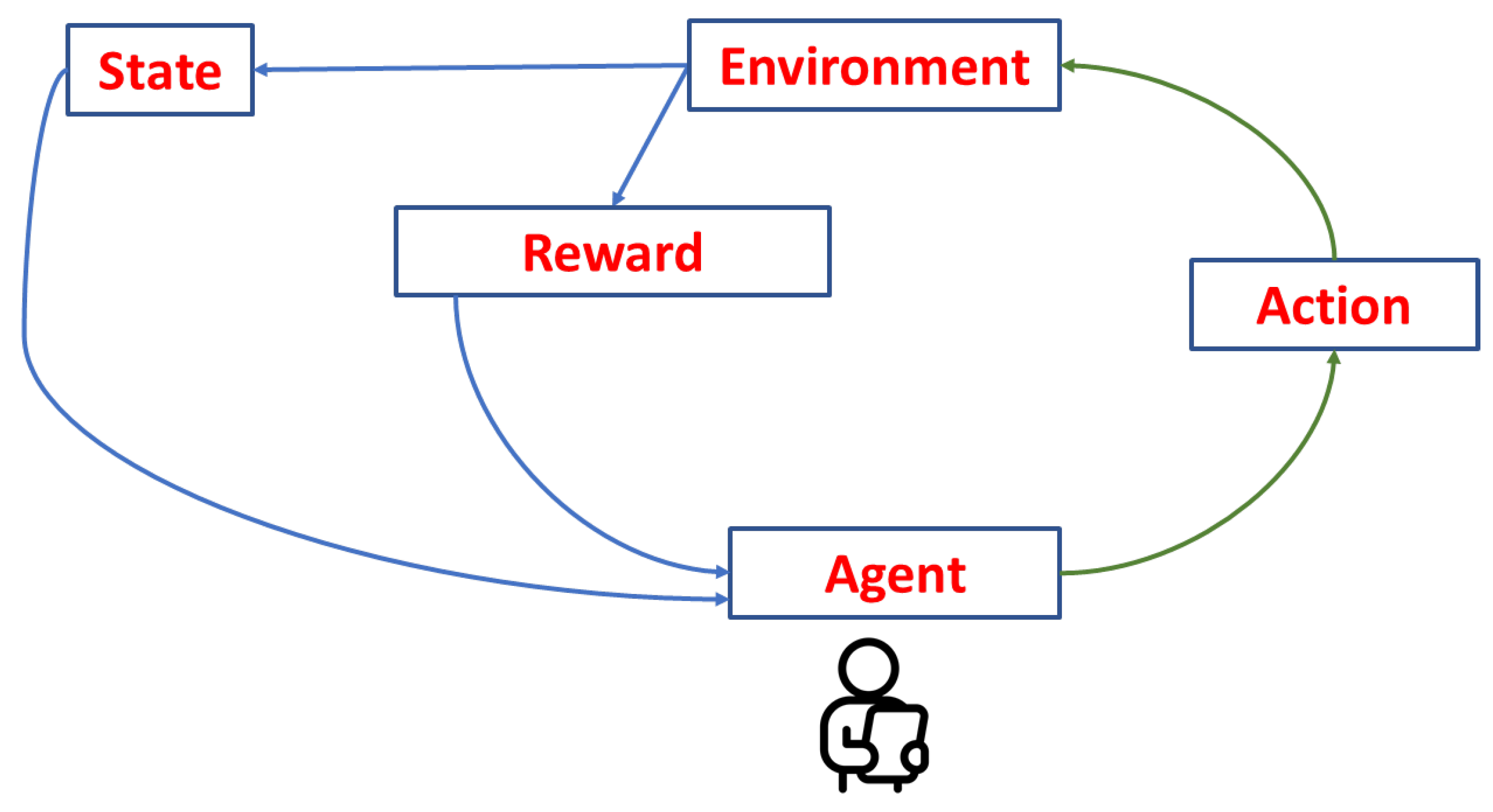
Figure 1 shows a simplified diagram of a typical reinforcement learning cycle, in which the agent observes the state of the environment, takes an action, receives a reward, and observes a new state again as a result of the action over the environment. Through this constant loop, the agent learns what it should do.

Figure 1. Basic learning cycle of reinforcement learning.

There are several reinforcement learning algorithms based on the principles described previously. However, in this study, TD3—which stands for Twin Delayed Deep Deterministic Policy Gradient [16]—was selected because it is designed to work with a continuous action space in dynamic environments, as is the case applied to the CWP.

The TD3 algorithm [17] is an improved version of the DDPG algorithm, a reinforcement learning algorithm that adopts a Double Deep Q Learning approach and employs an actor–critic mechanism to calculate target values for two Q functions. Compared to DDPG, the TD3 algorithm has the following improvements:

• Two critic networks are employed, each with a target network, resulting in a total of four networks.
• The delayed policy update strategy is employed, which updates the actor network within a certain period of time.
• Target policy smoothing is employed, which adds noise to the actor’s output when computing the target.

4. Reinforcement Learning Implementation

In reinforcement learning, the environment is a key element—as presented in Figure 1—where the agent interacts and achieves rewards. The environment can be tailored according to the specific case or based on existing tools. In the case presented in this paper, the environment was inspired and designed according to the method used in Gymnasium [18] for its collection of free environments.

Gymnasium is a Python library that allows the creation of environments to train reinforcement learning agents. As mentioned, the environment is fundamental because it defines what the agent can observe, what actions it can take, and how it is rewarded based on its behavior. Without a well-defined environment, the agent has no space to learn from. In the case described in this paper, a custom environment was created using Gymnasium based on real operational data. Each training episode spans a time period of that data, and the agent observes the state of the system, makes decisions (in this case, predictions), and receives a reward based on how close or far it is from the actual value.

The environment created according to the model that Gymnasium follows has the important advantages of having a clear structure, being easy to understand, and being able to connect with the algorithms of reinforcement learning. The procedure inside the environment for organizing data, structuring the episode, and calculating the reward is defined in a clear and systematic way. This is key for easily adapting the real-world working conditions of the CWP and ensuring that the agent learns consistently. 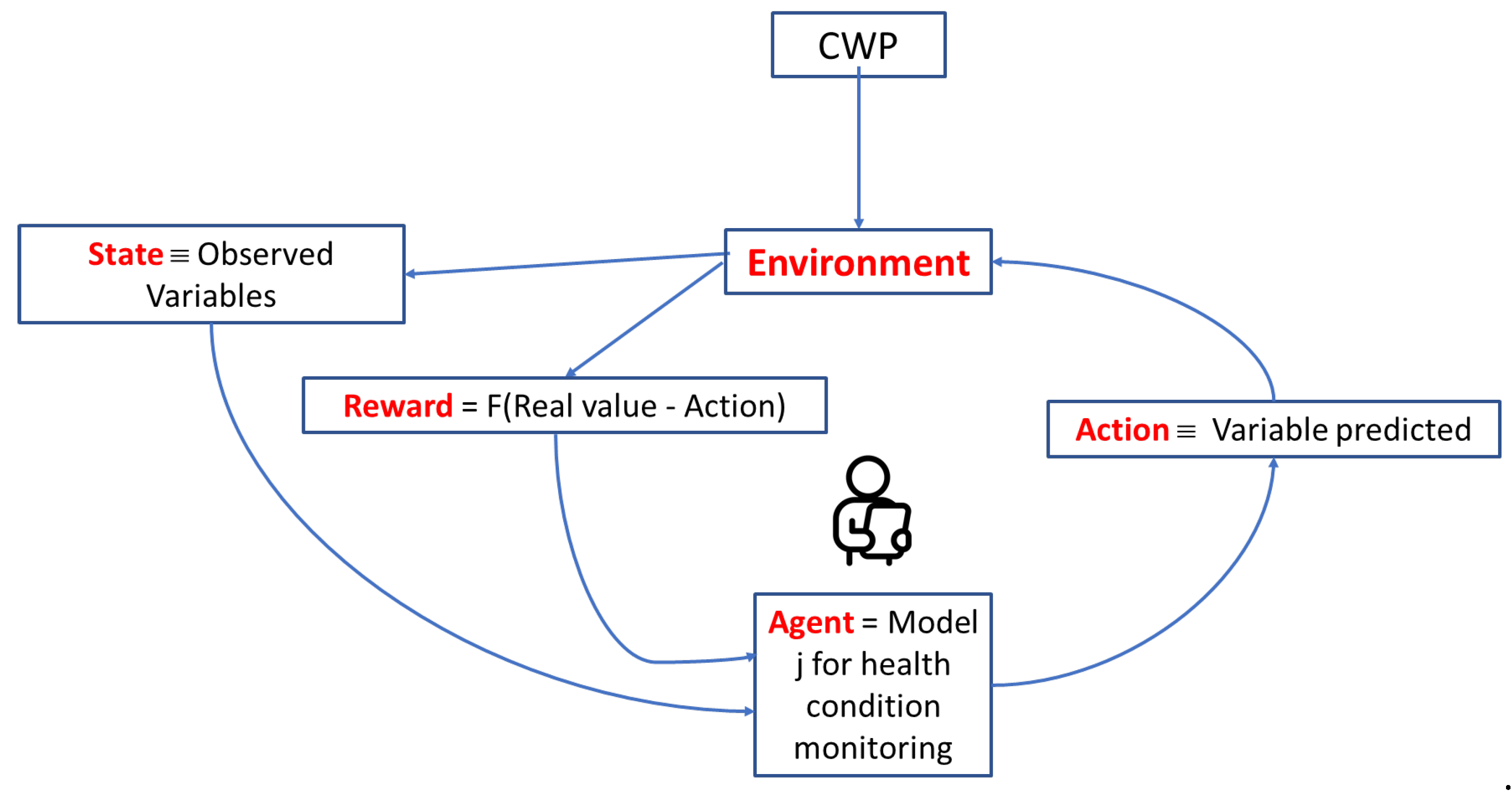Figure 2 presents the instantiation of Figure 1 for the case implemented.

Figure 2. Implemented reinforcement learning cycle.

In this paper, the Agent in Figure 2 corresponds to one of the several models suggested by the FMEA, developed to observe the presence or absence of symptoms of the particular failure mode that it monitors. It has to learn the usual relationships in normal behavior between several input variables collected by the pump’s SCADA system and some output variable that can raise an alert about a possible failure mode. The model to learn has to be valid for any working condition of the CWP.

The Agent observes the State that corresponds to its input variables and, according to its knowledge, makes an estimation of the value of the output variable as an Action.

The Environment knows the Action and compares its value with the real value that the agent should have obtained; the difference is the error between the real value and the predicted one. The Reward is obtained by a quadratic equation that depends on the error, with the following expression: Reward = −Action × (10 × error + 50 × error²). According to this, the reward is strongly negative when the error is large and near 0 when the error is small. The agent will try to maximize the reward, preventing actions with a negative reward or, equivalently, trying to obtain an error of 0.

The Reward and a new set of input variables selected as a new State stimulate the agent, starting the learning cycle once again.

Once the environment was created, a TD3 reinforcement learning algorithm was selected to build the models representing the Agent because it is oriented to problems with continuous action spaces, as is the case with the CWP. It was chosen from Stable-Baselines3 (SB3) [19], a library that includes ready-to-use implementations of several reinforcement learning algorithms. It is a very useful tool because it allows for focusing the effort on designing the environment and analyzing the results, without having to program each algorithm from scratch. It is also designed to work perfectly with environments created with Gymnasium, making everything seamless.

The learning process used in this paper consists of 500 episodes, each of 150 timesteps, a learning rate of 0.001, and a gamma value of 0.6. These hyperparameters were optimized through trial and error, a common practice in machine learning techniques.

In this study, the following software packages and versions were used: Python version 3.11.9, stable_baseline_3 version 2.7, gymnasium version 1.0, scikit_learn version 1.7.2, pandas version 2.3.3, numpy version 1.26.4, and matplotlib version 3.9.1.

5. Methodology Implemented to Monitor the CWP’s Health Condition

The general idea of the methodology is based on real data collected from the CWP, which is used in a training environment where models are constructed, learning how the CWP should behave under normal working conditions.

When designing the system, four years of CWP operation were available for applying the methodology proposed; the first year of data was used for training as a reference for the typical performance of the CWP, and the rest were used to observe the performance of the CWP with respect to the reference. The data were cleaned, removing those not valid for learning and testing.

After the cleaning step, the training dataset was fed into the customized environment created with Gymnasium, as mentioned before. The Agent observes real sequences of data of the pump’s operation during the first year, which in terms of reinforcement learning, are called episodes. The agent, trained with the TD3 algorithm from SB3, learns to predict the value that a given variable, which is key for monitoring the possible occurrence of a failure mode, should have, according to the inputs feeding the environment.

Once the model was trained using the first year of data available, the next available years were presented to the model, and its predictions were compared with the real ones measured at the CWP. This permits the detection of possible anomalies that can cause failures and allows the estimation of a stress indicator that can give an idea of the health condition, both providing very valuable information for maintenance purposes.

Details about this methodology can be found in the following subsections.

5.1. Data Preparation

The data used are based on real data recorded by the combined-cycle plant’s SCADA. In particular, for this study, the temporal evolution of various variables, such as temperatures, pressures, power, and flow rates, are measured at different points in the CWP jointly with the power generated by the gas turbine and steam turbine belonging to the combined cycle. The dataset available is extensive and contains useful information, but it also includes data that are not representative or could negatively affect training, so the first step was to carefully clean and prepare the data.

First, data periods in which the power plant was not operating at a rate above 5 MW—including startups and shutdowns—were eliminated due to transient conditions. To ensure this, the whole dataset was filtered, keeping only the samples in which both the gas turbine and steam turbine power levels were above 5 MW. Additional filtering was applied to eliminate extreme values or outliers that could distort learning.

This ensures that the data used reflect the usual operational conditions. Once this initial filter was applied, available data covering 4 years was sorted by date and divided temporally. The year 2020 was used as the training set, while data from subsequent years (2021 to 2023) were reserved for the validation phase. This separation ensures that the CWP’s performance during the whole training year is learned and how it behaves when faced with more recent situations is checked, with conditions that may have changed slightly compared to the training period.

Once the data were selected and cleaned, all variables were scaled. This allowed the signal ranges to be normalized between 0 and 1, which facilitated the training model and prevented certain variables from dominating others due to their numerically higher values. This normalization process is important because, if the data are not properly filtered, organized, and scaled, the agent could learn patterns that do not represent the actual CWP performance.

5.2. Learning Environment Design

As was mentioned before, the environment is one of the key components of reinforcement learning. Here, instead of using a generic or a pre-designed environment, a specific environment was created for each model responsible for monitoring if an anomaly that could cause a failure mode is present. This allows the agent to learn in an environment that reflects the working conditions of the CWP exactly. The use of the environment is quite straightforward. At each step, the agent receives as input an observation that includes the variables necessary to predict the target variable. According to the input received, the agent interacts with the environment, generating an action, which in this case is a prediction of the value of the output variable being modeled.

Once the prediction is made, the environment compares it with the actual value of the signal at that instant. Based on the error made, a reward is calculated: the closer the prediction is to the correct value, the greater the reward. This way of posing the problem allows the agent to learn to improve its accuracy over time, without the need to use labels or explicitly mark what constitutes a failure and what does not. It is based solely on its ability to give correct predictions.

Each training episode covers a complete time period of the data available to that model. At the end of the episode, the environment resets and returns to the beginning, allowing the agent to perform multiple passes through the same dataset and continue fine-tuning its behavior. This is especially useful when working with real data, as it allows the agent to take full advantage of it without having to generate synthetic data. Furthermore, the environment has been designed to be flexible so that it is easy to adapt to each model. Changing the target variable or input signals does not require modifying the entire environment structure, which allows different models to be trained without complications. This made the method used more manageable and easily extendable if the same approach were to be applied to other variables or other CWPs.

5.3. TD3 Algorithm Configuration

As mentioned, this algorithm was selected because it is especially able to work with continuous action spaces, as is the case in this system, where the agent must predict a numerical value at each step. Compared to simpler alternatives, TD3 offers greater stability during training and better results when the goal is to approximate a real-world behavioral function from data.

The same neural network architecture was used in all models and Agents; it has two hidden layers with 256 neurons each and is activated with ReLU functions (f(x) = max (0,x)). This configuration is quite common and works well in most cases.

A small amount of noise was also added to the predictions during training. This may seem counterproductive, but it is useful because it forces the model to explore different strategies before settling on one. The noise used is minimal so as to ensure the agent does not become stuck in a comfortable solution from the start that does not improve later.

This training process ensures that each model properly learns the normal behavior of its corresponding variable. From there, it will be able to detect behavior changes at any moment, which is precisely what this system aims to achieve.

5.4. Models Created

The system is made up of several independent models or Agents, each of which has been trained to predict the value of a specific system variable that characterizes possible failure mode symptoms. These variables are directly related to the pump performance and provide a clear reference as to how they should behave under normal conditions. Table 1 presents the FMEA developed that inspired the models that were built. This table consists of three columns: component or part of the CWP considered, the failure mode name, and the method or set of variables that can be used to detect if there are symptoms of the failure mode.

Table 1. CWP FMEA.

Component	Failure Mode	Detection Method
Pump electrical motor	Overload	Temperature of phases
	Phases imbalance	Imbalance of temperature in the phases
	Shortcircuit	Temperature of phases
	Cooling	Input/Output cooling air temperatures
Bearings (motor coupling side, opposite motor coupling side, thrust)	Lubrication	Bearing temperature
	Wear	Bearing radial vibration
		Bearing axial vibration
	Axis misalignement	Bearing axial/radial vibration
Pump	Pump performance degradation	Discharge pressure

In some cases, a single variable is enough to detect whether a failure mode is developing. For example, if a failure directly affects the discharge pressure or the temperature of a bearing, the model responsible for that variable only needs to detect a deviation to provide a clear signal. In other cases, the failure is not reflected in a single signal, but instead affects the behavior of several variables simultaneously. In these cases, the diagnosis is based on several different models, and the entire model is interpreted more completely.

The opposite also occurs: there are variables that are related to more than one failure mode. In these cases, the model that predicts that variable not only contributes to the diagnosis of a specific failure but also serves as a reference at various points in the system. This makes the system more efficient, since the same model can be used in different contexts without the need to repeat calculations or duplicate the structure. This organization allows for easy system adaptation. If new failure modes are detected in the future, or if the same logic is to be applied to another pump or at a different plant, it would be sufficient to train new models or redefine existing associations, without having to repeat everything from scratch.

A total of 21 models were built to cover the failure modes provided in Table 1 and use the data collected from the CWP. The power plant has four similar CWPs, and the models were developed for each. The presentation of all the results for all the models is outside this paper’s scope; therefore, only a few representative cases will be presented in the next section as examples of the benefits of the methodology applied.

It is important to keep in mind that each model represents the specific behavior of a particular pump; these are not generic models that can be applied interchangeably to any similar piece of equipment. If it is required to apply the same approach to another pump, it is necessary to retrain the models using their own operating data.

6. Examples of the Methodology Applied

The first example of application of the methodology described above is the evaluation of the health condition of the thrust bearing according to its temperature in one of the four pumps available in the power plant; in particular, CWP 4 was selected as an example. An agent was in charge of learning the relationship between the thrust bearing’s observed temperature and its working condition, which is represented by the temperature of one of the phases of the electrical motor and the discharge pressure of water, both characterizing the work of the pump, and by the power generated by the gas and steam turbines that represent the work demanded of the pump. Following the schema presented in Figure 2, the State observed corresponds to the values of the variables: temperature in one phase of the electrical motor, discharge pressure, and power from gas and steam turbines. The Action is the thrust bearing temperature predicted, and the Environment estimates a reward according to the error obtained and changes the State to a new one. This cycle is repeated in different steps per episode. During this process of learning, the agent is expected to collect better and better reward values. Figure 3 presents two instances of the learning process. The left column of the table corresponds to the beginning of the learning process (episode 4), where the mean reward at that moment was −308 (variable ep_rew_mean) and the losses in the actor and critic neural networks were 3.63 and 69, respectively. After 480 episodes (see right column of the table), the reward was improved to a value of −123, and the distance in losses between the two neural networks was closer than before; these facts demonstrate that the model is learning. The training time for this example was 18 min on a computer with an Intel(R) Core(TM) (Santa Clara, CA, USA) i7-4790 CPU @ 3.60 GHz 3.60 GHz, RAM: 8.00 GB, and Windows 11 Enterprise OS (Redmond, WA, USA).

Figure 3. Two instances of the learning process at the beginning (left column) and at the end (right column).

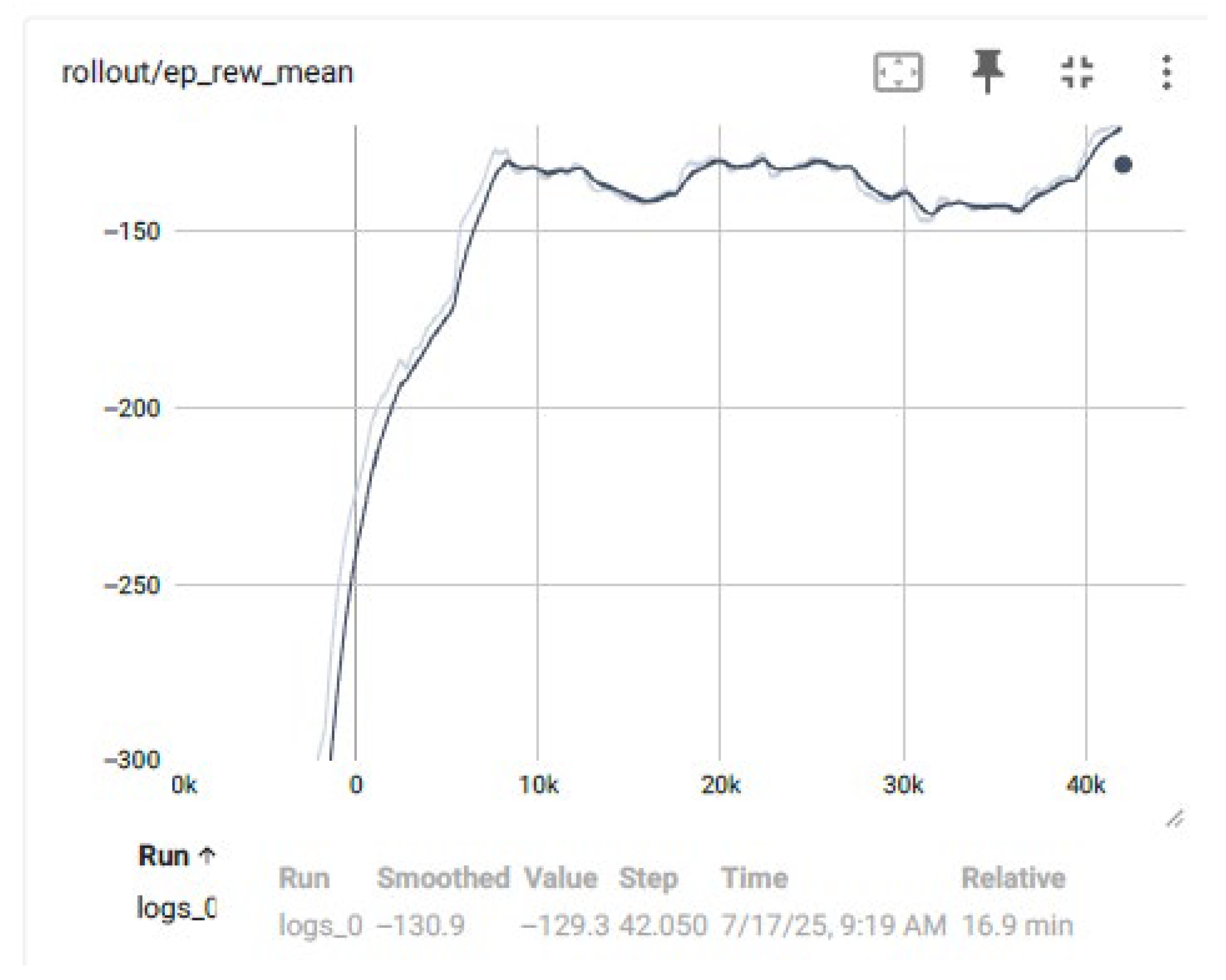
A more general perspective of the whole TD3 learning process is presented in Figure 4. It is observed how the reward improves when the number of steps per episode increases. The y-axis is the reward, and the x-axis is the steps of the loop. At the beginning, the negative value of the reward is high, but it decreases till its approximate stabilization, confirming that the Agent is learning and the model is improving.

Figure 4. Reward evolution during the reinforcement learning cycle.

When the Agent was fully trained, the quality of the model obtained was evaluated. Figure 5 shows the similarity of the real and predicted values for the training set from 2020.

Figure 5. Real and predicted values for the training dataset.

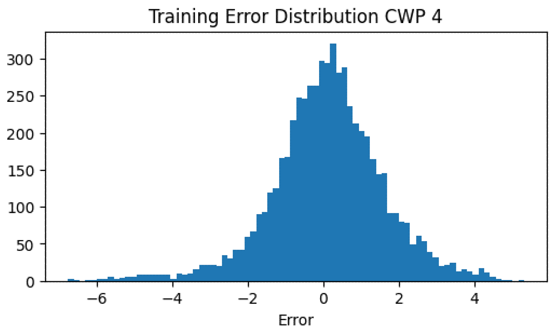
The mean value of the error obtained is −0.10 °C, with a standard deviation of 1.65 and RMSE value of 0.825. Figure 6 presents a histogram of the training error distribution that is centered around 0, a fact that agrees with the close approximation between the real and predicted values observed in Figure 5.

Figure 6. Distribution of the training error.

Even when the error is small, it has to be considered to reduce the possible number of false alarms if it is to be used for detecting an abnormal temperature in the pump’s thrust bearing. For this purpose, an upper confidence band for the error is defined covering 3 times the standard deviation observed for the training error, and is shown in Figure 7. A lower confidence band is not considered because it does not affect the possible failure mode due to abnormally high temperature. If three consecutive points are outside the upper band, this is considered to be a possible anomaly in the behavior expected. Figure 7 presents only a few non-representative points outside the confidence band, indicating good representation of normal values for the thrust bearing temperature during 2020 for CWP 4.

Figure 7. Training error observed and its confidence band.

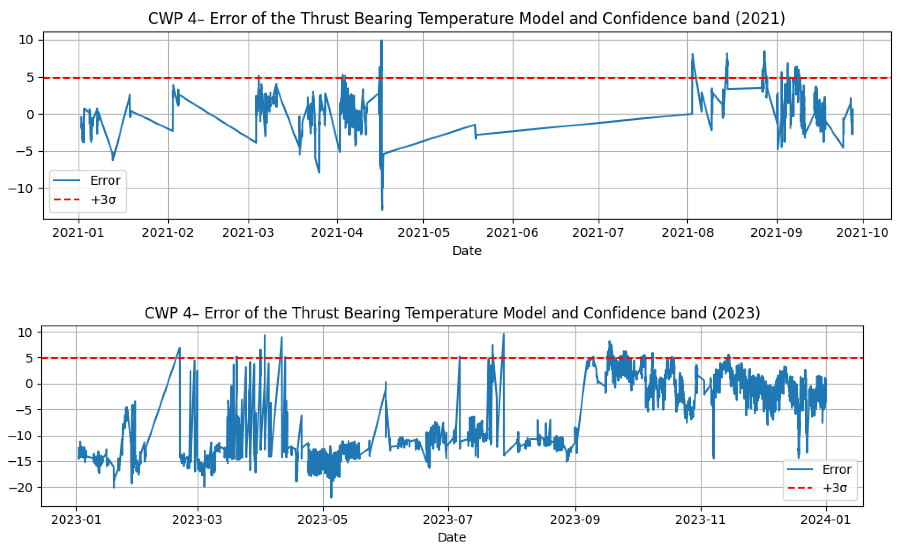
The model was tested with the subsequent years’ data in order to discover some possible anomaly in the thrust bearing temperature of CWP 4, but no abnormal values were found for this case. The prediction time was 20 s. Figure 8 presents the prediction error for the years 2021 and 2023 of the thrust bearing temperature using the model trained with the data from 2020. In the figure, no significant data are observed exceeding the confidence band, meaning that the temperature observed in 2021 and 2023 in the pump was similar to that corresponding to 2020, and no alarming degradation is observed in the pump’s health. Also, some discontinuity points were observed in 2021 because the pump was not working during some periods that year.

Figure 8. Test error observed and its confidence band in 2021 (top) and 2023 (bottom).

Once the models of normal relationships have been learned in the absence of symptoms of the failure modes that they monitor, they can be used to check for incoming new input values and whether the output variable has values within the confidence band. If a sustained period of time is observed during which the error is outside the confidence band, there is a risk that the failure mode that the model monitors will occur. This risk does not mean immediate failure, but now there is stress on the component that was not there before. In the method described here, a risk point appears when three of five consecutive new data samples are outside the confidence band. Monitoring the failure mode risk is extremely important for making decisions about maintenance assets, simultaneously saving time and resources while also keeping the assets in the best condition.

An example can better clarify the impact of the previous assertions about the benefits of failure mode and risk monitoring. Figure 9a–c shows the case of the model, abbreviated as M16, corresponding to the vibration observed in the radial direction on the opposite side of the coupling of the electrical motor to the pump, according to the pressure discharge of CWP 4 and the load generated by the gas and steam turbines. After learning the behavior from 2020 using the TD3 algorithm, as explained before, the new data from the period 2021 to 2025 are passed through the learned model. In Figure 9a, it is observed that the real and predicted values for the vibration studied were as expected until around the end of 2023, but an increasing deviation is observed from this date. This deviation of the error is better observed in the middle of Figure 9b, which also shows the sustained period of time during which the confidence band is exceeded. The cumulative value of the deviations exceeding the confidence band is obtained, which the authors call the “Cumulated Failure Mode Risk,” for which mathematical definitions can be found in references [6,20], also by the authors of this paper. Figure 9c reflects the evolution of this indicator over time. At the beginning of the time period represented, the value 0 indicates that CW4’s health is good due to this failure mode, and that the failure mode risk does not exist. However, this risk increases from the end of 2023 to the last date represented. The most important feature to observe is the slope of the trend because this can signal rapid degradation, which is key information for maintenance and operation crews.

Figure 9. (a). Example of health condition degradation in a CWP. Real vs. expected vibration for the operation mode observed. (b). Example of health condition degradation in a CWP. Error observed between real and predicted values and confidence band. (c). Example of health condition degradation in a CWP. Evolution of the Cumulated Failure Mode Risk or stress for M16.

Continuing with the case of CWP4 and the risk observed in Figure 9c, it could be questioned whether other vibration measurement points are presenting a similar risk or not. There are five models monitoring vibrations in CWP 4: thrust bearing axial vibration (named M19), radial and axial vibration on the opposite side of the electrical motor coupling to the pump (named M16 and M17, respectively), and radial and axial vibration on the side of the electrical motor (named M14 and M15, respectively). Figure 10 shows the evolution of the respective deviations or risks for all the models mentioned. In this figure, it is observed that there is no risk of the different failure modes monitored in the vibrations until mid-2022, where some small risks are observed in models M17 and M18. Also, during 2023, the other measurement points are affected, with a higher level of vibration with respect to the expected; however, their increase is contained and kept at very stable levels. The only important increasing trend in risk observed corresponds to M17, which is the radial vibration of the bearing on the opposite side of the electrical motor coupling to the pump. This provides important information for the maintenance crew to help them adapt planned maintenance according to the risk curves observed.

Figure 10. Example of CWP 4’s health condition based on vibrations.

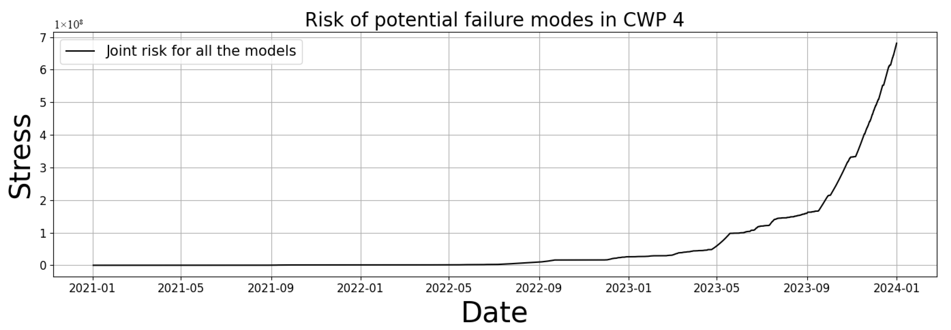
It could be useful at times to have a broader view of the failure mode risks in a complete risk curve before exploring the reasons for a possible increase in risks in depth. Figure 10 shows how a risk curve should be, combining all the risk curves presented in Figure 11.

Figure 11. Example of health condition degradation in a CWP.

7. Discussion

In this paper, a methodology is presented that is able to define the health condition of industrial components based on modeling the relationships between variables that can indicate the presence of a potential failure mode in an industrial component and those representing its working conditions. These relationships are learned by models built using the reinforcement learning algorithm named TD3. Reinforcement learning techniques are not usually applied in approaches like that proposed in this paper. Their successful application, as demonstrated in this paper, contributes to filling the knowledge gap in this field. One of the main advantages of reinforcement learning techniques is that they do not require large datasets for discovering the knowledge behind them. It is true that training this type of reinforcement learning model usually requires time periods of minutes (in the case presented, 18 min), but this can be reduced using GPUs. However, the errors obtained in training and testing are acceptable for the purposes of early anomaly detection of failure modes; for example, for the case presented in Figure 6, it can be observed that the error was ±2 °C, which is very low for the range of temperatures in the thrust bearing studied.

Other contributions of this paper are supported by the failure mode risk curves proposed as indicators of the health condition of industrial components. The models developed using the TD3 algorithm monitor if symptoms of deviation with respect to the normal behavior expected are observed. If they exist, the value of this deviation is used to estimate a risk indicator whose accumulated value gives a profile of failure mode progression that is extremely useful for making decisions for both maintenance and operation crews.

This study applies the methodology to real datasets of CWPs belonging to a combined-cycle power plant, and examples of the modeling and use of risk curves are presented and discussed. They have demonstrated the potential benefits of the method proposed. The same methodology has been applied to the other three CWPs in the power plant studied; however, only the results for CWP 4 are reported here to illustrate the proposed method. The prevention of catastrophic failure modes in any CWP can save a significant amount of money in maintenance and operation. Continuously monitoring the risk curves gives important feedback to the maintenance team that allows them to coordinate repairs according to the real-time condition of the component, leading to more effective maintenance and prolonging the life of the asset.

Additionally, the methodology described is general and not dependent on the example used. It can be easily extended to other industrial components where data on their functioning are available from a SCADA. In future extensions of this work, the impact of maintenance strategies will be analyzed through the change in the risk curves.

8. Conclusions

This study has demonstrated the feasibility of implementing reinforcement learning algorithms for detecting anomalies in industrial components. In particular, TD3 was selected due to its continuous nature, which facilitates learning through the actions to be taken. There are only a few publications in this area; therefore, this study contributes to filling this gap in the literature.

Also, the main features of a new methodology for evaluating the risks of failure modes have been presented. This is useful for guiding maintenance in the most efficient way, using the resources needed according to the real-time condition of assets. Beyond technical advantages, the methodology improves coordination between operation and maintenance teams by providing clear, real-time visualizations of risk and the impact of maintenance actions. The risk curves provide clear, quantitative insights into maintenance impacts, fostering a shared understanding of equipment conditions and priorities.