Accurate Seamless Vertical Handover Prediction Using Peephole LSTM Based on Light-GBM Algorithm in Heterogeneous Cellular Networks

Abstract

Present and future mobile networks combine wireless radio access technologies from multiple cellular network generations, all of which coexist. Seamless Vertical Handover (VH) decision-making is still a challenging issue in heterogeneous cellular networks due to the dynamic conditions of networks, different demands on QoS, and the latency of the handover process. Maintaining a very high-accuracy VH decision requires considering several network parameters. There is a trade-off between the gain of the VH accuracy and the corresponding latency in the computational complexity of the decision-making methods. This paper proposes a lightweight VH prediction DL strategy for 3G, 4G, and 5G networks based on the Light-Gradient Boosting Machine (LGBM) feature selection and Peephole Long Short-Term Memory (PLSTM) prediction model. For dense networks with large datasets and high-dimensional data, the combination of PLSTM and the fast feature selection LGBM, can reduce the computing complexity while preserving prediction accuracy and excellent performance levels. The proposed methods are evaluated using three case study scenarios using different feature selection thresholds. The performance evaluation is achieved by training and testing the proposed model, which shows an improvement using the proposed LGBM and PLSTM in terms of reducing the number of features by 64.28% and enhancing the VH accuracy prediction by 43.81% in Root Mean Squared Error (RMSE), and reducing the VH decision time of up to 51%. Furthermore, a network simulation using the proposed VH prediction algorithm shows an enhancement in overall network performance, with the number of successful VHs being 87%. Consequently, the data throughput is significantly enhanced.

1. Introduction

The proliferation of mobile networks is evidenced by the rise in user numbers and the adoption of contemporary technologies like the Internet of Things (IoT) [1,2]. Nevertheless, given the variety of applications and ways that have emerged from this ground-breaking explosion of wireless systems, a special technology built on a single infrastructure is required, one that can provide customers with excellent service quality in a range of scenarios. Future wireless systems will inevitably need to communicate via heterogeneous technologies to meet the vast requirements of such broad applications [3]. Without having to worry about the kind of network or the capabilities of the terminal, this trend can be very beneficial in enabling the service providers to deliver their network services to consumers efficiently. A Vertical Handover (VH) moves mobile terminals between different wireless networks [4]. VH is a key factor in providing smooth movement between wireless systems. Despite the fact that the conventional Received Signal Strength (RSS) algorithms have been used extensively for VH decision-making in telecom networks, in 5G environments their performance still has considerable limitations [5]. These limitations arise from a number of factors, the most important of which is the use of a single variable such as RSS. This eventually leads to incorrect decision making in complicated 5G areas, which are also influenced by factors like noise, interference, user speed, and cell load. Moreover, the unavailability of prediction for connection degradation before it happens, results in delays to handover decision or temporary loss of the connection [6]. Researchers have tried to devise a workable plan to reduce the handover delay. When a handover decision is made, switching to a different technology is still in progress. The prediction approach could be used to solve this problem. Since the VH prediction is considered a time series problem, the Long Short-Term Memory (LSTM) deep learning algorithm can be utilized for VH prediction. However, its learning capabilities can be degraded due to the short-term dependencies and temporal awareness in input data. Hence, the modified version with the Peephole connection of the LSTM addresses these issues. Now, although the Peephole Long Short-Term Memory (PLSTM) provides better accuracy compared to the traditional LSTM, it has a slightly complex structure resulting from the parameters of the additional connections. In the context of wireless VH, the decision time is one of the key factors that impact the network performance. Therefore, an efficient feature selection is required to reduce the overall model parameters, which leads to minimizing the decision time.

In this paper, a prediction technique is proposed using the PLSTM based on the Light-GBM Algorithm in heterogeneous cellular networks. The main contribution of this work is as follows:

(1)

Using a combination of the PLSTM and LGBM algorithms to provide more accurate predictions for VH decisions with less computational time complexity.

(2)

The proposed VH decision model is evaluated through a simulation scenario that mimics real network conditions, effectively demonstrating the model’s robustness, adaptability, and superior performance in ensuring seamless connectivity across heterogeneous wireless networks.

The structure of the paper is organized as follows. Section 2 presents the related work. Section 3 illustrates the background to the VH, along with the theoretical side of the proposed algorithms. Section 4 presents a brief description of the applied dataset. Section 5 contains the proposed algorithms. Section 6 includes the simulation results and discussion. Finally, Section 7 contains the conclusion of this work.

2. Related Works

Vertical Handover (VH) is a crucial component of user mobility in heterogeneous wireless networks since it directly impacts network performance in terms of data rate, packet latency, and the percentage of call blocking. Hence, VH decision strategies were the subject of extensive research studies. There are various varieties of these strategies, such as the traditional handover decision that typically relies on the values of multiple factors, such as power consumption, RSS, bandwidth, or a predetermined threshold of a particular parameter [7]. A method for making predictions employing a single threshold was put forth by utilizing the RSS value with filters such as Kalman and Fourier [8,9]. They assessed several filtering techniques for handover prediction. The vertical handover based on RSS, in which the network with the greatest RSS value is chosen among the available networks, was studied by the authors in [10,11]. However, a higher variation in the RSS value may lead to unnecessary handovers or even handover failures. Vertical Handover approaches have been investigated using AI Techniques, including Fuzzy Logic [12] and Neural networks [13,14,15].

A neuro-fuzzy controller was investigated in [16,17] to enhance the handover process in 5G heterogeneous networks. Three linguistic variable inputs on the signal intensity of the network were used in developing this controller. Additionally, the 5G heterogeneous network’s handover breakdown rate was reduced using the adaptive fuzzy interface structure, which improved QoS in the process and prevented pointless handovers. However, other useful parameters can be taken into consideration for increasing accuracy. The authors of [18,19] used edge computing to carry out vertical handovers of networks based on RSS. Compared to cloud computing [20], edge computing reduces latency by bringing data centers closer to users or mobile terminals. In [21], the authors suggested a handover decision-making algorithm that combines the dwelling time prediction approach with the methodology for order of preference to minimize the number of pointless handovers in 5G heterogeneous networks. The authors presented a stochastic geometric analysis scheme in [22,23] for small cell networks and user mobility. An approximation and theoretical statement are obtained for the anticipated frequency of handovers. Numerous research contributions address using Deep Learning (DL) and Machine Learning (ML) algorithms in VH decision-making in heterogeneous networks. The authors of [24] suggested using an artificial neural network and a Random Forest classifier on real-world sensor data gathered over three months by five smartphone users. To provide smooth vertical handovers, the trained models are implemented on smartphones and can accurately forecast Wi-Fi connection loss in advance. In [25], the handover algorithms were designed using Logistic Regression (LR) and Support Vector Machines (SVM). The simulation findings demonstrate that the LR- and SVM-based handover approaches perform better than the prior handover schemes; however, because these two methods have an inherent drawback in tackling the non-linear boundary classification problem, it may be difficult to enhance their handover accuracy further. In [26], the authors utilized multipath TCP to dynamically transition between various connectivity modes; the authors provide a data-driven method for smooth Wi-Fi/cellular handovers on smartphones that anticipate Wi-Fi connection loss. They used real-world sensor data to train an artificial neural network and a Random Forest classifier. The authors of the research studies presented in [27,28,29,30,31,32,33,34] focused on the application of Deep Learning (DL) as an assistant tool to improve the accuracy of VH. Likewise, further research studies have been conducted based on the application of Machine Learning (ML) as in [35,36,37,38].

Unlike the prior studies that have mostly focused on one or a small number of choice criteria in their search for an intelligent plan. This research broadens the scope of the handover decision criteria to include a wide range of factors, including network requirements, device characteristics, and application and service requirements. Additionally, it uses DL and lightweight ML tools to construct accurate vertical handover management at minimum decision latency in real-time services

3. Background

The main components of this research are highlighted concisely in the following subsections.

3.1. Vertical Handover Processes

Wireless systems of the present and future generations will comprise a heterogeneous environment with various access network technologies that have differing properties, as illustrated in Figure 1. Nevertheless, the most important thing is to integrate these disparate networks so that mobile wireless devices can connect to them seamlessly [39]. A network node that performs a vertical handover switches the connectivity type it employs to access a supporting infrastructure, usually to facilitate node mobility. Vertical handover involves these three fundamental processes as demonstrated in Figure 2 [40,41]: (1) Initiation, (2) Decision-Making, and (3) Execution (Transfer of Connection). The mobile terminal, or network controller, has to know which wireless networks are reachable to initiate the process. Using a vertical handover decision algorithm, the decision step selects the access point based on appropriate performance predefined indicators (e.g., RSSI, network connection time, available bandwidth, power consumption, cost, security level, and user preferences). The goals of this step are to choose a superior alternative connection and determine the precise moment for a handover. The execution step activates the network switching mechanism. This may also entail authentication processes, database searches, node reconfiguration, connection association, and signaling.

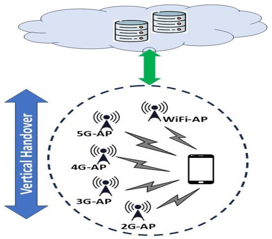
Figure 1. Vertical Handover of Mobile User in a Heterogeneous Network.

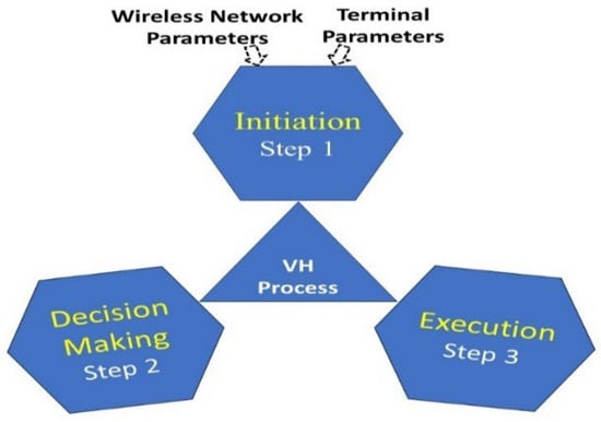
Figure 2. Main Vertical Handover Process.

3.2. Feature Selection Using the LGBM Algorithm

Feature selection is a crucial step in machine learning and data analysis that involves identifying and retaining the most relevant features from a dataset while removing those that are redundant, irrelevant, or noisy. The primary goal of feature selection is to improve the performance of a model by focusing on the features that contribute the most to making accurate predictions. By eliminating unnecessary features, the model becomes simpler, which can lead to better generalization when applied to new, unseen data. A distributed, high-performance gradient boosting framework called Light Gradient Boosting Machine was developed by Microsoft Research Institute in 2017 [42]. For applications where speed and scalability are crucial, such as classification, regression, and ranking, LGBM performs very well [43]. It systematically constructs models by fusing several ineffective learners, usually decision trees, to produce a powerful prediction model. Each successive model in the series aims to fix the mistakes made by the earlier models. It is a different model of growing gradient trees using light gradient augmentation decisions. While the other decision tree branches vertically in the analysis process, LGBM branches horizontally over the leaves. The decision tree continues to branch over the leaf with the largest delta, wilting. There are services such as performing fast transactions, processing larger data, and performing analyses with less computer memory compared to other incremental models. Another advantage of the LGBM model is that it does not require processes such as one-hot encoding to analyze data numerically with categorical variables. LGBM gives better results on large datasets than other models on the dataset, as overfitting measures are easier to find in different datasets. It has been noticed that the LGBM model is 20 times faster than the Support Vector Machine (SVM) model in finding the data [44].

The significance of feature qualities is determined by applying the LGBM algorithm. This can be accomplished by taking into account the following factors: the total number of times the feature is used to split in all decision trees; the feature elements are sorted in descending order; the feature elements are started from the complete set of sample features; and the decision to exclude is made based on the accuracy of the result [45]. In this manner, feature selection is achieved by looping through the feature that currently has the lowest degree of relevance. In general, LGBM can be used for both classification and regression. In this work, a modified version of LGBM is used for feature selection. The mathematical formulation of the LGBM feature selection algorithm is explained as follows. The objective function can be expressed in (1).

$$Obj\_fun=L(\vartheta ,\widehat{\vartheta })+\mu (f)$$

(1)

where $L(\vartheta$,$\widehat{\vartheta }$) represents the loss function; $\mu \left(f\right)$ denotes the regularization term. The LGBM tree construction is achieved sequentially to reduce the errors of the former trees. LGBM separates the data according to a feature $k$ that is taken into consideration at each phase. The objective is to identify the feature that optimizes the loss function. The following represents the gain (or loss decrease) from splitting on feature $k$ at a node $s$:

$$G\left(k,s\right)={\displaystyle \frac{1}{2}}\left({\displaystyle \frac{{\beta }_l^2}{H_l+\propto }}+{\displaystyle \frac{{\beta }_r^2}{H_r+\propto }}+{\displaystyle \frac{{\left({\beta }_l+{\beta }_r\right)}^2}{H_l+H_r+\propto }}\right)-\delta$$

(2)

where $\beta$ and $H$ represent the derivatives of the loss function of right and left child nodes; $\propto$: the big leaf weights are penalized by this regularization parameter. δ: it is used for regularization that penalizes the tree’s leaf count.

Then the importance of the selected feature $k$ from the total number of features $n$ is calculated by summing the gain across all splits that used the feature $k$:

$$Important\left(k\right)={\sum }_{n\in Z_k}G\left(k,s\right)$$

(3)

where $Z_k$ is the collection of all nodes that were split using the feature $k$. Features with the greatest significance ratings are deemed appropriate for the task once the model has been trained. The significance score can direct the choice of features via either thresholding or ranking. Figure 3 illustrates the flow diagram of LGBM feature selection.

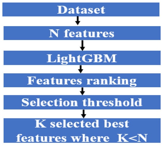
Figure 3. LGBM feature selection technique.

The key steps for the LGBM algorithm with input $x$ of training data and (∝,δ) hyperparameters to generate the output of the trained LGBM model and the features of importance scores are summarized as follows:

• Step 1: Initialize LGBM model parameters
• Step 2: Iterate to build decision trees to compute the gradients (1st order and 2nd order)
• Step 3: Find the best feature by calculating the right and left child nodes, then find the gain for split nodes.
• Step 4: Updating the importance feature to obtain the best feature.
• Step 5: Adding the recently trained tree to the model.
• Step 6: Choosing features and considering their importance based on thresholding or ranking.
• Step 7: Return the chosen features and their importance accordingly.

LGBM offers many advantages in feature selection in machine learning models. One of the main advantages is the ability to handle large amounts of data efficiently, making it suitable for high-quality, multi-feature data. LGBM automatically ranks features based on their importance, allowing for easy identification of the most influential variables. This process not only speeds up the model training by reducing the feature space but also enhances the model’s performance by eliminating irrelevant or redundant features. Additionally, the Exclusive Feature Bundling (EFB) and Gradient-based One-Sided Sampling (GOSS) methods of the LGBM can both enhance the selection process by preserving accuracy and lowering computational complexity. This results in a fast and scalable model that can be successfully applied to a wide range of tasks from classification to regression, without the risk of overfitting. In comparison to other versions of Gradient Boosting methods, such as GBM and XGBoost, LGBM has superior advantages, as illustrated in Table 1.

Table 1. A Comparison Between Multiple Gradient Boosting-Based Feature Selection Methods [46,47].

Feature	GBM	XGBoost	LGBM
Speed of evaluation	Relatively slow	Slower than LGBM	Very fast due to the use of histogram splitting
Accuracy of feature ranking	Medium to low	High	High, especially for large data
Flexibility in handling redundant features	Weak	Good	Very good
Support for missing values	Does not automatically support	Good	Excellent
Custom scoring control	Limited	Flexible	Flexible
Stability across folds	Unstable	Good	Stable with imbalanced data
Best suited for feature selection in big data	Not suitable	Very good	Best

It is worth stating that LGBM uses two straightforward methods to determine feature importance. First (split count): It keeps track of how frequently each feature is used in the trees to reach a decision. Second (gain): It measures the extent to which each feature contributes to increased accuracy when the data is split. Hence, the feature’s importance increases with its usefulness or frequency of use.

LGBM was considered for feature selection because of its lightweight tree structure and histogram technology, which allow it to train more quickly and use less memory. In comparison to Random Forest, it offers strong tools for managing class imbalances, is effective with large-dimensional data, and performs on par with or better than XGBoost in numerous applications. LGBM is appropriate for attaining optimal performance because it permits significant parameter adjustments.

3.3. Peephole LSTM Algorithm

PLSTM is a new architecture that has been developed by making new additions to the traditional LSTM. In [48,49], the authors added peephole connections to the LSTM and enabled the information stored in the cell to affect the entry and forget gate. Thus, they were able to influence whether the data would be stored, changed, or not, and whether there would be new incoming information in the output information. In other words, it is an improvement on the conventional LSTM design that permits direct influence of the gates by the cell state. PLSTM enables the gates to access the cell state during the prediction process. Hence, in comparison to traditional LSTM, this feature in PLSTM increases the model’s sensitivity to fast wireless channel fluctuations and enhances the vertical handover decision’s timing accuracy, making it more appropriate for applications that demand real-time response and network condition adaptation. The key differences between the traditional LSTM and the Peephole LSTM are demonstrated in Table 2 [50,51].

Table 2. A comparison between the LSTM and Peephole LSTM.

Feature	LSTM	Peephole LSTM
Structure of Gates	Input Gate, Forget Gate, Output Gate	Input Gate, Forget Gate, Output Gate with peephole connections
Connections of Peephole	No peephole connections	Peephole connections allow gates to access the current cell state directly
Interaction of cell state	Gates do not directly access the cell state	Gates have direct access to the cell state, enhancing feedback
Computation Complexity	Less complex with fewer parameters	Slightly more complex due to additional parameters introduced by peephole connections
Uses	General sequence prediction tasks (NLP, time series)	Useful in tasks requiring precise timing and control (e.g., speech recognition)
Performance	Effective for most tasks with long-term dependencies	Can potentially improve performance where finer control over gates is beneficial

It is worth mentioning that in comparison to GRU, the PLSTM retains information for longer periods of time, provides better training stability in volatile data, and is less computationally expensive than BiLSTM, which necessitates forward and backward traversal. Without appreciably increasing training time or structural complexity. Hence, PLSTM offers a workable compromise between modeling power and precise time-tracing patterns and therefore is considered in this work for VH prediction.

Based on the comparison illustrated in Table 2, the PLSTM outweighs the traditional LSTM in terms of accuracy; therefore, it is considered in this work as a VH decision model. With selected features, the peephole LSTM can achieve a low-latency, lightweight architecture that can make accurate predictions in real-time VH decisions in resource-constrained environments. Feature selection guaranteed computational efficiency, and the peephole mechanism provided improved temporal sensitivity for signal fluctuations. The mathematical expressions of the Peephole LSTM approach are illustrated in Appendix A [49]. Figure 4 shows Peephole connections, which connect each controlling gate to the preceding memory cell.

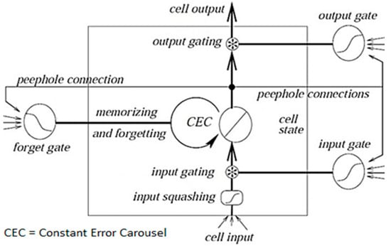
Figure 4. General block diagram of standard Peephole LSTM architecture [47].

Peephole: from the value in memory to the forget and sigmoid functions at the gate. The data in the new cell state is connected to the sigmoid function at the exit gate. In the diagram above, peepholes have been added to all doors. In another version, the entrance and forget door are combined. In this way, the decision of the information to forget and newly add is taken together, rather than separately. Algorithm 1 demonstrates the pseudocode of the PLSTM algorithm.

Algorithm 1: (Peephole LSTM) [49]
Input = network initialization: ${\sigma }_{c_j^v}$ = ${\widehat{\sigma }}_{c_j^v}=0$, $d\sigma =0,$$u=\widehat{u}=0$; forward pass: $u=$ current external input, $u=\widehat{u}$, ${\sigma }_{c_j^v}$ = ${\widehat{\sigma }}_{c_j^v}$; B = no. of memory blocks; ${\sigma }_j$ = no. of memory cells per block.
Output = VH Occurrence
1:	For j = 1 to B
2:	{
3:	Input gates calculations according to Equation (A1)
4:	Forget gates calculations according to Equation (A2)
5:	Cell states calculations using Equations (A3) and (A4)
6:	Activation of output gate calculation according to Equation (A5)
7:	For $v$ = 1 to ${\sigma }_j$
8:	{
9:	Cell output calculations according to Equation (A6)
10:	Output unit calculations according to Equation (A7)
11:	Partial derivatives for input and forget gates using Equations (8) and (9)
12:	}   //end loop of cells
13:	}   //end loop of memory blocks
14:	End

4. Dataset Description

The applied dataset, named “5G Dataset with Channel and Context Metrics”, was developed by an Irish mobile operator providing a 5G trace dataset [52]. The two mobility patterns, static and mobile, as well as the two application patterns, video streaming and file downloads, are used to create the dataset. The dataset includes throughput data, context, cell, and channel-related parameters, as well as client-side cellular key performance indicators. These statistics are produced by a popular network monitoring app for unrooted Android phones. Therefore, this becomes a significant publicly accessible dataset that includes context, channel, and throughput data for 5G networks. The attributes that went into creating the dataset are displayed in Table 3.

Table 3. The attributes of the dataset [52].

No.	Feature	Description
1	Longitude	Mobile device’s GPS coordinates
2	Latitude	Mobile device’s GPS coordinates
3	Speed	The Mobility speed of a mobile device
4	Cell-Id	Serving as a mobile device’s cell
5	UL_bitrate	Uplink bitrate (UL_bitrate) the device’s (application layer) measurement of the uplink rate
6	State	The state in which the download is happening. It can have one of two values: D (downloading) or I (idle).
7	ServingCell_Distance	Distance to the serving cell
8	SNR	The Signal-to-Noise Ratio (SNR) value
9	RSRQ	Reference Signal Received Quality (RSRQ) represents a ratio between RSRP and Received Signal Strength Indicator (RSSI).
10	RSRP (Reference Signal Received Power)	Value for RSRP.
11	RSSI	value for RSSI.
12	CQI	value for a mobile device’s Channel Quality Indicator (CQI).
13	NRxRSRQ	RSRQ and RSRP values for the neighboring cell, where NR denotes 5G New Radio.
14	NRxRSRP

5. The Proposed VH Prediction Using Plstm and Lgbm Algorithms

The overall design model is depicted in Figure 5. The steps of the operation procedure consist of two parts. First, feature selection using LGBM to reduce the number of features by selecting the best-related features, including channel-related metrics, context-related metrics, cell-related metrics, and throughput information. Second, the handover decision model represented by the PLSTM, which is a lightweight version of the traditional LSTM to minimize the inference time.

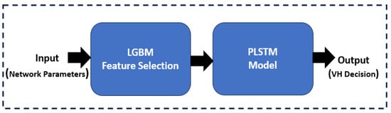
Figure 5. Operation of the proposed methods.

The flow diagram of the proposed PLSTM/LGBM method is illustrated in Figure 6.

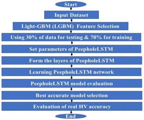
Figure 6. The flow diagram of the proposed PLSTM/LGBM.

The traditional RSS-based VH method is used as a baseline for comparison in order to validate the suggested PLSTM/LGBM-based VH approach. In real-world wireless deployments, the RSS-based scheme is the most commonly used threshold-driven mechanism, where VH decisions are made exclusively based on received signal strength conditions. To demonstrate the advantages of integrating predictive intelligence into the decision-making process by contrasting the proposed model with this common baseline. Compared to traditional RSS-only methods, this allows for a more proactive handover strategy that makes use of gradient-boosted inference and temporal feature learning, improving stability and minimizing needless handovers. The mathematical description [53] of the ${RSS}_{VH}$ is illustrated as follows:

$${RSS}_{VH}={Tx}_P-P{L}_0-10 ϵ lo{g}_{10}\left({\displaystyle \frac{\mathrm{R}}{D_0}}\right)+\mathrm{z}$$

(4)

where ${Tx}_P$ is the base station’s transmit power, $P{L}_0$ denotes the path loss at a reference distance $D_0$, The path loss exponent is denoted by $ϵ$, R is the separation distance between the base station and the mobile user, and $\mathrm{z}$ is a Gaussian random variable with zero mean that represents the fading due to shadows.

To determine handover, the current RSS is then compared to the dynamic RSS threshold [54] ${RSS}_{VH-Th}$ which can be determined as follows:

$${RSS}_{VH-Th}={RSS}_{VH-min}+10 ϵ lo{g}_{10}\left({\displaystyle \frac{R}{R-r}}\right)+\mathrm{z}$$

(5)

where ${RSS}_{VH-min}$ is the minimum RSS required to stay communicating with the base station, $r$ shortest path between the base station boundary and the location where VH is activated.

Now, it is important to predict the traveling time (dwell time) ${dw}_t$ to avoid superfluous VH and failures [54]. It is a key method in vertical handover to make a decision whether a mobile device should be shifted to another network or not. Predicted dwell time, as expressed in Equation (6) allows a device to forecast its stay in a new network’s coverage area. This is certain to assist in reducing the number of unnecessary handovers, minimizing the occurrence of failure during handover, and providing a good Quality of Service (QoS) by taking into account criteria such as signal strength and network conditions.

$${dw}_t={\displaystyle \frac{R^2-l^2+M^2{\left(t_c-t_e\right)}^2}{M^2\left(t_c-t_e\right)}}$$

(6)

where $l$ denotes the separation between the base station and the RSS sample point, $M$ is the node mobility speed, $t_c$ is RSS measurement sampling time, $t_e$ is the time that the user entered the coverage area of the base station.

Now, the three variables of Equations (4)–(6) (${RSS}_{VH}$, ${RSS}_{VH-Th}$, ${dw}_t$) will participate in logical and sequential interactions. The ${RSS}_{VH}$ is calculated and compared with the dynamic ${RSS}_{VH-Th}$ to determine the VH trigger point. Then, in the case of ${RSS}_{VH} \le {RSS}_{VH-Th}$, the handover process will proceed when the ${dw}_t>T_{TH}$, where $T_{TH}$ is a predefined minimum threshold time that the user has to stay in the target network for the handover to be beneficial. The pseudocode of the RSS based VH is described in Algorithm 2.

Algorithm 2: RSS-based VH.
Input = network initialization: $R$, $l,$ $t_c,$ $t_e$, $T_{TH}$.
Output = Decision [Trigger_VH, No_VH]
1:	${∆}_t = t_c-t_e$   //Calculate time difference
2:	If $({∆}_t\le 0$)
3:	Return No_VH
4:	Else
5:	Calculate dwell time (${dw}_t$)//Equation (6)
6:	If (${RSS}_{VH}$ $\le$ ${RSS}_{VH-Th}$)   //Check RSS condition
7:	If (${dw}_t)>$ $T_{TH}$,)
8:	Return Trigger_VH
9:	Else
10:	Return No_VH
11:	Else
12:	Return No_VH
13:	End

6. Performance Evaluation and Discussion

Figure 7 illustrates the evaluation methodology of the proposed system. The performed evaluation is split into two primary sections. First, the evaluation is focused on the accuracy of the proposed algorithm, PLSTM/LGBM, using the RMSE evaluation metric. Then the second part is focused on evaluating a real wireless network using the number of successful VH and the network downlink throughput as evaluation metrics. The network simulation parameter settings are illustrated in Table 4.

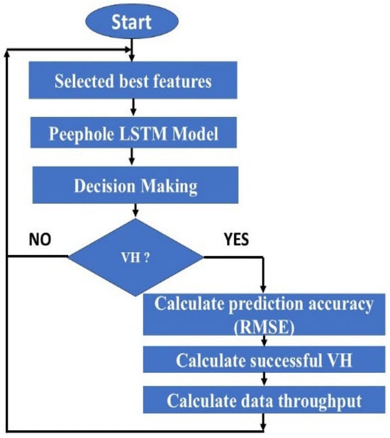
Figure 7. The evaluation methodology of the proposed system.

Table 4. Simulation parameter settings.

Parameter	Value/Description
Directions for data transmission	Downlink
Type of network	3G, 4G, 5G
Bandwidth	5 MHz, 20 MHz, 100 MHz
Frequency	1.9 GHz, 2.3 GHz, 4.8 GHz
User mobility	0–100 km/h
Type of areas	Urban
System specifications	Processor: 2.3 GHz Intel Core i7, 8 GB of DDR4 RAM, Framework: Python, 64-bit Windows 10

First of all, the dataset features are sorted based on their importance score concerning the target feature using the LGBM method, as shown in Figure 8.

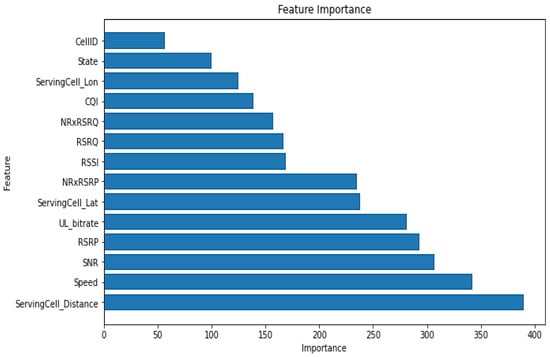
Figure 8. Feature importance using LGBM (DL_bitrate).

The threshold “feature importance” for selecting the best features based on the importance score is shown in Table 5. Regarding feature selection, the thresholds are manually determined after multiple trials to ensure the selection of influential and effective features. Features with low influence, or those that increased response time without improving performance, were excluded to ensure a lightweight and effective VH decision model.

Table 5. Threshold value and number of selected features.

Threshold	Number of Features
>250	5
>150	10
>0	14

The strategy of the LGBM for selecting the best features is accomplished by using Feature Importance Analysis, in which the weights acquired during training are used to evaluate each feature’s contribution to the accuracy of the model. The most significant features are then chosen to lower complexity and enhance model performance after the features are arranged in decreasing order of significance. The best set of features directly related to the Vertical Handover prediction process can be obtained by using LGBM techniques like gain or split importance to ascertain each feature’s influence on the ultimate choice.

The values of importance thresholds shown in Table 5 are derived from observations of the data’s practical and empirical behaviors. These thresholds are used to separate the values of selected features (e.g., the distance and SNR) into various levels that correspond to different network states. Hence, strong instability or extreme variability are frequently indicated by values above 0, while the moderate variability is indicated by regions larger than 150, and the low or stable state is indicated by values greater than 250. A more accurate VH decision is made possible by this division, which facilitates the model’s ability to differentiate between degrees of link improvement or deterioration.

Four evaluation metrics are used in this work with 10-fold cross validation. First, the Root Mean Squared Error (RMSE) method is used to calculate the difference between the root square of actual and expected expenditures. The RMSE, as shown in Equation (7), measures the absolute degree of fit. Thus, the spread of the residuals is calculated by RMSE.

$$RMSE=\sqrt{\left({\displaystyle \frac{1}{e}}\right){\sum }_{i=1}^e{(a_i-{\widehat{a}}_i)}^2}$$

(7)

where $a_i$ denotes the actual data, ${\widehat{a}}_i$ refers to the predicted data, $e$ represents the number of observations.

The second evaluation metric, as in Equation (8), is represented by the Mean Absolute Error (MAE), which determines the mean of the absolute differences between the actual values and the predicted values.

$$MAE=\left({\displaystyle \frac{1}{e}}\right){\sum }_{i=1}^e\left|a_i-{\widehat{a}}_i\right|$$

(8)

Third, the coefficient of determination or R-squared $R^2$ metric, as demonstrated in Equation (9), is applied. It is worth stating that the $R^2$ quantifies how well the predicted values fit or approximate the data. It is the proportion of variance in the dependent variable that can be explained by the independent variables.

$$R^2=1-{\displaystyle \frac{\left(\frac{1}{e}\right)\sum _{i=1}^e{\left(a_i-{\widehat{a}}_i\right)}^2}{\left(\frac{1}{e}\right)\sum _{i=1}^e{(a_i-\overline{a_i})}^2}}$$

(9)

where $\overline{a_i}$ is the mean of all the values.

Finally, the confidence interval is calculated based on Equation (10) [55]. A confidence interval has the advantage of offering an approximate estimate of the range that, based on sample data, is likely to contain the true value of a parameter (e.g., the mean) in a statistical population. It offers a level of assurance (95%) regarding this estimate’s accuracy [56].

$$\mathrm{C}\mathrm{o}\mathrm{n}\mathrm{f}\mathrm{i}\mathrm{d}\mathrm{e}\mathrm{n}\mathrm{c}\mathrm{e} \mathrm{I}\mathrm{n}\mathrm{t}\mathrm{e}\mathrm{r}\mathrm{v}\mathrm{a}\mathrm{l}=\phi \mp \zeta {({\displaystyle \frac{\mathrm{P}\left(1-\mathrm{P}\right)}{e}})}^{0.5}$$

(10)

where $\phi$ represents the accuracy of the model, $\zeta$ is the z-score level, $\mathrm{P}$ is the percentage of successes in samples. The model hyperparameters shown in Table 6 are selected through comprehensive trial experiments to ensure optimal model performance. The process of tuning the hyperparameters went through a meticulous process of fine-tuning to achieve the best possible performance from the model that was proposed. Part of the process was to thoroughly test a number of different values for primary parameters such as the learning rate, dropout rate, number of layers, and hidden units. The learning rate test had several values taken from a set range of [10⁻⁵, 10⁻²] and the value that resulted in the quickest convergence and least validation loss was chosen. The dropout rate was accepted from a range of [0.2, 0.5] to prevent overfitting thus maintaining the model’s accuracy at an acceptable level.

Table 6. Values of Hyperparameters.

Hyperparameters	Value
Number of PLSTM Layers	2
Hidden Units	64
Dropout Rate	0.2
Sequence Length	10
Batch Size	32
Learning Rate	0.001
Optimizer	Adam
Number of Epochs	150
Activation function	Rectified Linear Unit (ReLU)
Loss function	RMSE

Likewise, the suggested model in connection with real-time adaptation to the changing network conditions has been created to adjust to these changes in a dynamic manner through two primary ways. The first method is by the continuous Input Update where the model depends on real-time network data (like RSRP, SINR, user speed, and cell load). These values are updated in real time right before each new prediction and thus the system is able to make an up-to-date, accurate VH decision. Second, through Online Fine-Tuning. The model is capable of incremental learning when there are continuous changes in the network environment. That way, the weight can be slowly adjusted according to the new data without needing to go through a full retraining process. This approach allows the system to keep low latency while, at the same time, enhancing the accuracy of the decisions made under changing network conditions.

The proposed PLSTM architecture consists of two PLSTM layers with 64 hidden units. The RMSE is used as a loss function for training the proposed PLSTM.

The model is trained using different combinations of selected features using the LGBM method. The loss function of the model during the training process for 150 epochs is shown in Figure 9.

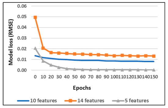
Figure 9. The model training loss (RMSE) vs. the number of epochs.

Then, the evaluation results of the model when applying the testing dataset in terms of RMSE are shown in Table 7 for different numbers of selected features.

Table 7. PLSTM model evaluation results.

Features	RMSE	MAE	R2	Confidence Interval (95%)	$\mathit{p}$ Value
14 (ALL)	9.86	8.37	0.76	8.87, 10.85	0.0032
10	8.47	7.4	0.82	7.62, 9.32	0.00001
5	5.54	4.69	0.91	4.99, 6.09	0.00001

Based on the results illustrated in Table 7, it can be noticed that the dataset with five features selected by LGBM achieved the best performance in terms of prediction RMSE, MAE, and R². Regarding the p-value, a smaller p-value indicates stronger evidence, which is often used to assess statistical significance.

As the feature set reduced, the model’s performance improved. Moderate accuracy was obtained when all 14 features were used (R² = 0.76), but better results were obtained when less informative variables were eliminated. Prediction error decreased and performance improved (R² = 0.82) with 10 features. Only five features yielded the best results, with the lowest RMSE (5.54), lowest MAE (4.69), and highest R² = 0.91, suggesting that the most predictive value was found in a small subset of features. More model consistency was demonstrated by narrowing confidence intervals with fewer features. Strong statistical significance (p < 0.01) was shown by all configurations.

This results in a reduction rate of 64.28% from the total number of features, which can be calculated as follows.

$$Reduction Rate={\displaystyle \frac{Number of Removed Features}{\mathrm{T}\mathrm{o}\mathrm{t}\mathrm{a}\mathrm{l} \mathrm{N}\mathrm{u}\mathrm{m}\mathrm{b}\mathrm{e}\mathrm{r} \mathrm{o}\mathrm{f} \mathrm{F}\mathrm{e}\mathrm{a}\mathrm{t}\mathrm{u}\mathrm{r}\mathrm{e}\mathrm{s}}}100\%$$

(11)

The selection of features in this study, as shown in Table 8, was carried out through LGBM, which allocated high weight (importance) to the features SNR, RSRP, UL_bitrate, Mobility Speed, and Cell Distance because of their direct impact on radio conditions and mobility context. Irrelevant or weak features such as GPS coordinates, Cell ID, and so on, were rejected to avoid noise and reduce computational complexity. Combining LGBM feature ranking with peephole LSTM temporal prediction significantly reduced computational requirements and latency, making it an excellent solution for real-time vertical handover decision-making in mobile networks.

Table 8. The importance of the selected features using LGBM.

No.	Feature	Importance
1	ServingCell_Distance	390
2	Speed	340
3	SNR	310
4	RSRP	290
5	UL_bitrate	280

Figure 10 shows the difference between the actual and predicted values of data rate using the proposed PLSTM/LGBM method.

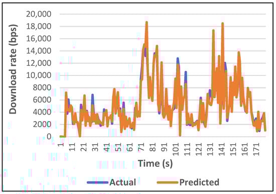
Figure 10. Actual vs. predicted values of DL_bitrate using the model with best-selected features by LGBM.

The decision time (inference time) of the proposed PLSTM is calculated with and without the feature section LGBM method, as shown in Table 9. The introduction of LGBM has a noticeable impact on reducing the VH decision time.

Table 9. VH decision time.

Method	No. Features	Decision Time (ms)
PLSTM	14	37
PLSTM-LGBM	5	18

The next part of the simulation tests the number of successful VHs and the user’s data throughput using the proposed algorithm, using the predefined parameter settings shown in Table 4. To verify the effectiveness of the proposed model, the network simulation is conducted using the network environment shown in Table 10. One user is considered in the simulation to testify to the performance of the proposed algorithm. The single user simplifies investigating the effect of distance and mobility on throughput and the count of successful handovers. The user starts moving along the path from BS-location 0 to location 1000 m in a straight line.

Table 10. Simulation network environment.

BS-Location (m)	BS-Type	Coverage Range (m)
0	5G-BS1	300
300	4G-BS1	400
500	5G-BS2	300
700	4G-BS2	400
1000	3G-BS1	600

The Received Signal Strength (RSS)-based algorithm is used for comparison to the suggested approach, which is extensively utilized as a conventional vertical handover algorithm and bases handover decisions mostly on the strength of the signal received from various networks. Figure 11 shows the effectiveness of the proposed PLSTM in terms of several successful VH compared to the traditional technique that merely relies on the RSS value. The noticeable performance of proposed approach can be clearly observed.

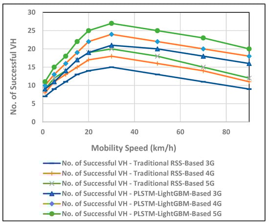
Figure 11. Evaluating the performance of the proposed VH in terms of successful VH with the mobility speed.

The proposed PLSTM-LGBM VH algorithm distinguishes itself from the traditional RSS-based methods by predicting the optimal handover times with low latency and preventing handover failures, especially at high mobility speeds. It maintains continuous connectivity and optimized throughput, whereas the traditional method can cause premature or delayed handovers, resulting in dropped connections and reduced performance.

The proposed PLSTM-LGBM-based VH algorithm increases data rates, minimizes delay, and provides seamless transitions across networks by predicting handovers based on mobility speed, as illustrated in Figure 12. The conventional RSS-based approach, on the other hand, performs poorly as the speed at which the node is traveling increases, which translates to either late switching or unnecessary handovers, thus affecting throughput. With speed predictive handovers, the proposed VH method escalates data throughput, reduces delays, and ensures seamless transitions across networks. In contrast, the more traditional RSS-based methods suffer from higher speeds, where either switching is delayed or handovers occur unnecessarily, thus affecting throughput.

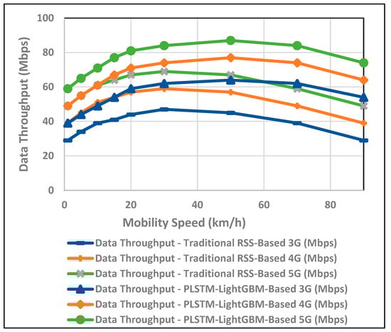
Figure 12. Evaluating the performance of the proposed VH in terms of data throughput with the mobility speed.

The PLSTM-LGBM-based VH algorithm is intended to make the best performance of handoffs into a more seamless and reliable process by accurately determining the switchover between networks when a user has moved far enough distance toward the BS, as shown in Figure 13. When the distance between the user and the BS increases, traditional RSS-based approaches would cause the user to initiate a handover either too early or too late, resulting in increased failure rates and a diminished quality of connectivity.

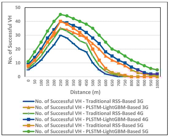
Figure 13. Evaluating the performance of the proposed VH in terms of successful VH, with the distance from the access point.

By predicting the ideal handover points based on user movement away from the access point, the proposed PLSTM-LGBM based VH algorithm serves to ensure connectivity continuity throughout networks, while securing enhanced data throughput. Conversely, an early or delayed handover under the conventional RSS-based paradigm may result in a throughput drop with users moving far away from the access point, leading to inefficiency and poorer performance in the networks, as can be noticed in Figure 14.

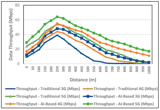
Figure 14. Evaluating the performance of the proposed VH in terms of data throughput with the distance from the access point.

In summary, the obtained simulation results with proposed PLSTM-LGBM VH outperformed the traditional RSS-based VH mothed in different network scenarios of 3G, 4G and 5G. The final simulation test was conducted to demonstrate the VH between different technologies for one of the selected features (e.g., RSRP) in the time domain, as shown in Figure 15.

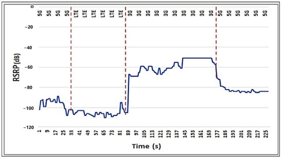
Figure 15. VH process for RSRP feature.

Consequently, the performance is better under the new algorithm. This, due to increasing prediction accuracy, leads to a successful VH process, improving the network performance. Where the feature selection and training process are performed initially, then the trained model of PLSTM is utilized to predict the VH. It is worth stating that to forecast future network circumstances, the proposed DL algorithm can be trained on previous data (such as signal strength, user mobility, and network congestion). With the use of this predictive capacity, the algorithm can forecast when a handover will be advantageous and prevent repeated switching brought on by sporadic fluctuations in signal strength. Hence, this can reduce the number of Ping-Pong useless handovers.

7. Conclusions

Handover is the process of moving a running data session from one core network-connected channel to another. Mobility and user preferences are important considerations here. This research aims to address the issue of users switching networks in heterogeneous integrated networks. The proposed algorithm provides high VH prediction accuracy using the Peephole LSTM deep learning method, with the lower computational complexity achieved by the LGBM feature selection method. The suggested system could make use of Radio Access Networks (RAN) and Multi-access Edge Computing (MEC) to implement VH decisions at the network side. Network-side VH decision-making is therefore appropriate for large-scale IoT over 5G since it guarantees scalability, policy control, and energy efficiency. Comprehensive evaluation scenarios are performed to achieve the best VH decision accuracy of 5.54 in terms of RMSE with the lowest model complexity, represented by using only five features, where removing irrelevant features by the LGBM method leads to an increase in the model performance. The evaluation results show the impact of the proposed HV algorithm on the network performance in terms of increasing successful VHs and data throughput. Further research work could be focused on the correlation between the vertical and horizontal handover to gain better network performance. Additionally, to gain better real-world urban conditions, such as interference, load balancing, and dynamic cell overlaps, future work would expand to multi-user simulations. Furthermore, it can investigate the possibility of automating the feature selection step via instructive techniques such as nested cross-validation or model-based feature selection for the sake of reproducibility and generalization.

References

- Gzar, D.A.; Mahmood, A.M.; Al-Adilee, M.K.A. Recent trends of smart agricultural systems based on Internet of Things technology: A survey. Comput. Electr. Eng. 2022, 104, 108453. [Google Scholar] [CrossRef]
- Al-Falahy, N.; Alani, O.Y.K. The impact of base station antennas configuration on the performance of millimetre wave 5G networks. In Proceedings of the 2017 Ninth International Conference on Ubiquitous and Future Networks (ICUFN), Milan, Italy, 4–7 July 2017; IEEE: Piscataway, NI, USA, 2017; pp. 636–641. [Google Scholar] [CrossRef]
- Albonda, H.D. Distributed Reinforcement Learning-based Seamless Multi-Connectivity Solution for Heterogeneous 5GNR and Wi-Fi Networks. Int. J. Intell. Eng. Syst. 2024, 17, 365–376. [Google Scholar] [CrossRef]
- Malik, A.A.; Jamshed, M.A.; Nauman, A.; Iqbal, A.; Shakeel, A.; Hussain, R. Performance evaluation of handover triggering condition estimation using mobility models in heterogeneous mobile networks. IET Netw. 2024, 13, 291–300. [Google Scholar] [CrossRef]
- Kareem, A.R.; Mahmood, A.M.; Al-Falahy, N. Performance Evaluation of IPTV Zapping Time Reduction Using Edge Processing of Fog RAN. Math. Model. Eng. Probl. 2022, 9, 928–936. [Google Scholar] [CrossRef]
- Hosny, K.M.; Khashaba, M.M.; Khedr, W.I.; Amer, F.A. New vertical handover prediction schemes for LTE-WLAN heterogeneous networks. PLoS ONE 2019, 14, e0215334. [Google Scholar] [CrossRef]
- Talebi, S.P.; Werner, S. Distributed Kalman filtering: Consensus, diffusion, and mixed. In Proceedings of the 2018 IEEE Conference on Control Technology and Applications (CCTA), Copenhagen, Denmark, 21–24 August 2018; IEEE: Piscataway, NI, USA, 2018; pp. 1126–1132. [Google Scholar] [CrossRef]
- Golchi, M.M.; Motameni, H. Evaluation of the improved particle swarm optimization algorithm efficiency inward peer to peer video streaming. Comput. Netw. 2018, 142, 64–75. [Google Scholar] [CrossRef]
- Ren, G.; Zhao, J.; Qu, H. A user mobility pattern based vertical handoff decision algorithm in cellular-WLAN integrated networks. In Proceedings of the 2016 2nd IEEE International Conference on Computer and Communications (ICCC), Chengdu, China, 14–17 October 2016; IEEE: Piscataway, NI, USA, 2016; pp. 1550–1554. [Google Scholar] [CrossRef]
- Agrawal, A.; Jeyakumar, A.; Pareek, N. Comparison between vertical handoff algorithms for heterogeneous wireless networks. In Proceedings of the 2016 International Conference on Communication and Signal Processing (ICCSP), Melmaruvathur, India, 6–8 April 2016; IEEE: Piscataway, NI, USA, 2016; pp. 1370–1373. [Google Scholar] [CrossRef]
- Gaur, A.S.; Budakoti, J.; Lung, C.H. Vertical handover decision for mobile IoT edge gateway using multi-criteria and fuzzy logic techniques. Adv. Internet Things 2020, 10, 57. [Google Scholar] [CrossRef]
- Patil, M.B.; Patil, R. A network controlled vertical handoff mechanism for heterogeneous wireless network using optimized support vector neural network. Int. J. Pervasive Comput. Commun. 2023, 19, 23–42. [Google Scholar] [CrossRef]
- Vilakazi, M.; Olwal, T.O.; Mfupe, L.P.; Lysko, A.A. Vertical handover algorithm in OpenAirInterface and neural network for 4G and 5G base stations. In Proceedings of the 2024 International Conference on Information Networking (ICOIN), Ho Chi Minh City, Vietnam, 17–19 January 2024; IEEE: Piscataway, NI, USA, 2024; pp. 126–131. [Google Scholar] [CrossRef]
- Tan, X.; Chen, G.; Sun, H. Vertical handover algorithm based on multi-attribute and neural network in heterogeneous integrated network. EURASIP J. Wirel. Commun. Netw. 2020, 2020, 202. [Google Scholar] [CrossRef]
- Semenova, O.; Semenov, A.; Voitsekhovska, O. Neuro-fuzzy controller for handover operation in 5G heterogeneous networks. In Proceedings of the 2019 3rd International Conference on Advanced Information and Communications Technologies (AICT), Lviv, Ukraine, 2–6 July 2019; IEEE: Piscataway, NI, USA, 2019; pp. 382–386. [Google Scholar] [CrossRef]
- Kiran, K.; Rao, D.R. Analytical review and study on various vertical handover management technologies in 5G heterogeneous network. Infocommun. J. 2022, 14, 28–38. [Google Scholar] [CrossRef]
- Maleki, H.; Başaran, M.; Durak-Ata, L. Handover-enabled dynamic computation offloading for vehicular edge computing networks. IEEE Trans. Veh. Technol. 2023, 72, 9394–9405. [Google Scholar] [CrossRef]
- Alkaabi, S.R.; Gregory, M.A.; Li, S. Multi-access edge computing handover strategies, management, and challenges: A review. IEEE Access 2024, 12, 4660–4673. [Google Scholar] [CrossRef]
- Goh, M.I.; Mbulwa, A.I.; Yew, H.T.; Kiring, A.; Chung, S.K.; Farzamnia, A.; Chekima, A.; Haldar, M.K. Handover decision-making algorithm for 5G heterogeneous networks. Electronics 2023, 12, 2384. [Google Scholar] [CrossRef]
- Mahmood, A.M.; Al-Yasiri, A.; Alani, O.Y. A new processing approach for reducing computational complexity in cloud-RAN mobile networks. IEEE Access 2017, 6, 6927–6946. [Google Scholar] [CrossRef]
- Duong, T.M.; Kwon, S. Vertical handover analysis for randomly deployed small cells in heterogeneous networks. IEEE Trans. Wirel. Commun. 2020, 19, 2282–2292. [Google Scholar] [CrossRef]
- Bao, W.; Liang, B. Stochastic geometric analysis of user mobility in heterogeneous wireless networks. IEEE J. Sel. Areas Commun. 2015, 33, 2212–2225. [Google Scholar] [CrossRef]
- Rehman, A.U.; Roslee, M.B.; Jun Jiat, T. A survey of handover management in mobile HetNets: Current challenges and future directions. Appl. Sci. 2023, 13, 3367. [Google Scholar] [CrossRef]
- Ma, G.; Parthiban, R.; Karmakar, N. An artificial neural network-based handover scheme for hybrid lifi networks. IEEE Access 2022, 10, 130350–130358. [Google Scholar] [CrossRef]
- Cervantes-Bazán, J.V.; Cuevas-Rasgado, A.D.; Rojas-Cárdenas, L.M.; Lazcano-Salas, S.; García-Lamont, F.; Soriano, L.A.; Rubio, J.d.J.; Pacheco, J. Proactive cross-layer framework based on classification techniques for handover decision on WLAN environments. Electronics 2022, 11, 712. [Google Scholar] [CrossRef]
- Höchst, J.; Sterz, A.; Frömmgen, A.; Stohr, D.; Steinmetz, R.; Freisleben, B. Learning Wi-Fi connection loss predictions for seamless vertical handovers using multipath TCP. In Proceedings of the 2019 IEEE 44th Conference on Local Computer Networks (LCN), Osnabrueck, Germany, 14–17 October 2019; IEEE: Piscataway, NI, USA, 2019; pp. 18–25. [Google Scholar] [CrossRef]
- Paropkari, R.A.; Thantharate, A.; Beard, C. Deep-mobility: A deep learning approach for an efficient and reliable 5g handover. In Proceedings of the 2022 International Conference on Wireless Communications Signal Processing and Networking (WiSPNET), Chennai, India, 24–26 March 2022; IEEE: Piscataway, NI, USA, 2022; pp. 244–250. [Google Scholar] [CrossRef]
- Kapadia, P.; Seet, B.C. Multi-Tier Cellular Handover with Multi-Access Edge Computing and Deep Learning. Telecom 2021, 2, 446–471. [Google Scholar] [CrossRef]
- Kapadia, P. 5G Multi-Tier Handover with Multi-Access Edge Computing: A Deep Learning Approach. Ph.D. Thesis, Auckland University of Technology, Auckland, New Zealand, 2021. [Google Scholar]
- Zhang, Z.; Hou, Y.; Hui, P.S.; Sun, C. Deep Learning Based Handover for High-Speed Connected Vehicles in Ultra-Dense Networks. In Proceedings of the 2024 IEEE Vehicular Networking Conference (VNC), Kobe, Japan, 29–31 May 2024; IEEE: Piscataway, NI, USA, 2024; pp. 290–296. [Google Scholar] [CrossRef]
- Nguyen, K.N.; Takizawa, K. Deep Learning-Based Proactive Physical Layer Handover using Cameras for Indoor Environment. In Proceedings of the 2024 IEEE 21st Consumer Communications & Networking Conference (CCNC), Las Vegas, NV, USA, 6–9 January 2024; IEEE: Piscataway, NI, USA, 2024; pp. 364–367. [Google Scholar] [CrossRef]
- Kayikci, S.; Unnisa, N.; Das, A.; Kanna, S.R.; Murthy, M.Y.B.; Preetha, N.N.; Brammya, G. Deep learning with game theory assisted vertical handover optimization in a heterogeneous network. Int. J. Artif. Intell. Tools 2023, 32, 2350012. [Google Scholar] [CrossRef]
- Mollel, M.S.; Abubakar, A.I.; Ozturk, M.; Kaijage, S.; Kisangiri, M.; Zoha, A.; Imran, M.A.; Abbasi, Q.H. Intelligent handover decision scheme using double deep reinforcement learning. Phys. Commun. 2020, 42, 101133. [Google Scholar] [CrossRef]
- Wang, L.; Han, D.; Zhang, M.; Wang, D.; Zhang, Z. Deep reinforcement learning-based adaptive handover mechanism for VLC in a hybrid 6G network architecture. IEEE Access 2021, 9, 87241–87250. [Google Scholar] [CrossRef]
- Khoder, R.; Naja, R.; Ismail, S.; Mouawad, N.; Tohme, S. Vertical Handover Decision using Machine Learning in Vehicular Platooning. In Proceedings of the 2021 3rd IEEE Middle East and North Africa COMMunications Conference (MENACOMM), Agadir, Morocco, 3–5 December 2021; IEEE: Piscataway, NI, USA, 2021; pp. 60–64. [Google Scholar] [CrossRef]
- Mitnala, V.N.; Reed, M.J.; Kegel, I.; Bicknell, J. Avoiding handover interruptions in pervasive communication applications through machine learning. In Proceedings of the 2021 IEEE International Conference and Expo on Real Time Communications at IIT (RTC), Chicago, IL, USA, 12–14 October 2021; IEEE: Piscataway, NI, USA, 2021; pp. 1–8. [Google Scholar] [CrossRef]
- Priyanka, A.; Gauthamarayathirumal, P.; Chandrasekar, C. Machine learning algorithms in proactive decision making for handover management from 5G & beyond 5G. Egypt. Inform. J. 2023, 24, 100389. [Google Scholar] [CrossRef]
- Aydin, T.; Rodosek, G.D. Machine Learning Based Predictive Handover in Unmanned Aerial Systems Communication. In Proceedings of the 2023 IEEE/AIAA 42nd Digital Avionics Systems Conference (DASC), Barcelona, Spain, 1–5 October 2023; IEEE: Piscataway, NI, USA, 2023; pp. 1–5. [Google Scholar] [CrossRef]
- Chakraborty, T.; Hossain, M.S.; Atiquzzaman, M. A testbed implementation of hybrid decision model based seamless lightweight vertical handover. In Proceedings of the 2017 IEEE International Conference on Communications (ICC), Paris, France, 21–25 May 2017; IEEE: Piscataway, NI, USA, 2017; pp. 1–6. [Google Scholar] [CrossRef]
- Al-Rubaye, A. Vertical Handover Management with Quality of Service Support. Ph.D. Thesis, Technische Universität Ilmenau, Ilmenau, Germany, 2017. [Google Scholar]
- Khattab, O.; Alani, O. I am 4 vho: New approach to improve seamless vertical hanover in heterogeneous wireless networks. arXiv 2013, arXiv:1306.1448. [Google Scholar] [CrossRef]
- Ke, G.; Meng, Q.; Finley, T.; Wang, T.; Chen, W.; Ma, W.; Ye, Q.; Liu, T.Y. LGBM: A highly efficient gradient boosting decision tree. Advances in neural information processing systems. In Proceedings of the 31st Conference on Neural Information Processing Systems (NIPS 2017), Long Beach, CA, USA, 4–9 December 2017. [Google Scholar]
- Sinha, B.B.; Ahsan, M.; Dhanalakshmi, R. LGBM empowered by whale optimization for thyroid disease detection. Int. J. Inf. Technol. 2023, 15, 2053–2062. [Google Scholar] [CrossRef]
- Xi, X. The role of LGBM model in management efficiency enhancement of listed agricultural companies. Appl. Math. Nonlinear Sci. 2023, 9, 1–14. [Google Scholar] [CrossRef]
- Liao, H.; Zhang, X.; Zhao, C.; Chen, Y.; Zeng, X.; Li, H. LGBM: An efficient and accurate method for predicting pregnancy diseases. J. Obstet. Gynaecol. 2022, 42, 620–629. [Google Scholar] [CrossRef]
- Florek, P.; Zagdański, A. Benchmarking state-of-the-art gradient boosting algorithms for classification. arXiv 2023, arXiv:2305.17094. [Google Scholar] [CrossRef]
- Boldini, D.; Grisoni, F.; Kuhn, D.; Friedrich, L.; Sieber, S.A. Practical guidelines for the use of gradient boosting for molecular property prediction. J. Cheminformatics 2023, 15, 73. [Google Scholar] [CrossRef]
- Essai Ali, M.H.; Abdellah, A.R.; Atallah, H.A.; Ahmed, G.S.; Muthanna, A.; Koucheryavy, A. Deep learning peephole LSTM neural network-based channel state estimators for OFDM 5G and beyond networks. Mathematics 2023, 11, 3386. [Google Scholar] [CrossRef]
- Gers, F.A.; Schraudolph, N.N.; Schmidhuber, J. Learning precise timing with LSTM recurrent networks. J. Mach. Learn. Res. 2002, 3, 115–143. [Google Scholar]
- Greff, K.; Srivastava, R.K.; Koutník, J.; Steunebrink, B.R.; Schmidhuber, J. LSTM: A search space odyssey. IEEE Trans. Neural Netw. Learn. Syst. 2016, 28, 2222–2232. [Google Scholar] [CrossRef] [PubMed]
- Ma, T.; Liang, Y.; Cong, M.; Yao, N.; Wang, K. Remaining Useful Life Prediction Based on LSTM with Peephole for PEMFC. SAE Tech. Paper 2022, 2022-01-7037. [Google Scholar] [CrossRef]
- Raca, D.; Leahy, D.; Sreenan, C.J.; Quinlan, J.J. Beyond throughput, the next generation: A 5G dataset with channel and context metrics. In Proceedings of the 11th ACM Multimedia Systems Conference, Istanbul, Turkey, 8–11 June 2020; pp. 303–308. [Google Scholar] [CrossRef]
- Yew, H.T.; Chekima, A.; Kiring, A.; Mbulwa, A.I.; Dargham, J.A.; Chung, S.K. RSS based vertical handover schemes in heterogeneous wireless networks: Past, present & future. In Proceedings of the 2020 IEEE 2nd International Conference on Artificial Intelligence in Engineering and Technology (IICAIET), Kota Kinabalu, Malaysia, 26–27 September 2020; IEEE: Piscataway, NI, USA, 2020; pp. 1–5. [Google Scholar]
- Gavali, V.S.; Patil, J.K. A study of RSS based vertical handover decision algorithms. Int. J. Eng. Res. Technol. 2015, 4, 825–827. [Google Scholar]
- Nasser, A.R.; Alani, O.Y. Investigation of Multiple Hybrid Deep Learning Models for Accurate and Optimized Network Slicing. Computers 2025, 14, 174. [Google Scholar] [CrossRef]
- Shan, G. Accurate confidence intervals for proportion in studies with clustered binary outcome. Stat. Methods Med. Res. 2020, 29, 3006–3018. [Google Scholar] [CrossRef]
Disclaimer/Publisher’s Note: The statements, opinions and data contained in all publications are solely those of the individual author(s) and contributor(s) and not of MDPI and/or the editor(s). MDPI and/or the editor(s) disclaim responsibility for any injury to people or property resulting from any ideas, methods, instructions or products referred to in the content. |
© 2025 by the authors. Licensee MDPI, Basel, Switzerland. This article is an open access article distributed under the terms and conditions of the Creative Commons Attribution (CC BY) license (https://creativecommons.org/licenses/by/4.0/).