EEGT: Energy Efficient Grid-Based Routing Protocol in Wireless Sensor Networks for IoT Applications

Abstract

The Internet of Things (IoT) integrates different advanced technologies in which a wireless sensor network (WSN) with many smart micro-sensor nodes is an important portion of building various IoT applications such as smart agriculture systems, smart healthcare systems, smart home or monitoring environments, etc. However, the limited energy resources of sensors and the harsh properties of the WSN deployment environment make routing a challenging task. To defeat this routing quandary, an energy-efficient routing protocol based on grid cells (EEGT) is proposed in this study to improve the lifespan of WSN-based IoT applications. In EEGT, the whole network region is separated into virtual grid cells (clusters) at which the number of sensor nodes is balanced among cells. Then, a cluster head node (CHN) is chosen according to the residual energy and the distance between the sink and nodes in each cell. Moreover, to determine the paths for data delivery inside the cell with small energy utilization, the Kruskal algorithm is applied to connect nodes in each cell and their CHN into a minimum spanning tree (MST). Further, the ant colony algorithm is also used to find the paths of transmitting data packets from CHNs to the sink (outside cell) to reduce energy utilization. The simulation results show that the performance of EEGT is better than the three existing protocols, which are LEACH-C (low energy adaptive clustering hierarchy), PEGASIS (power-efficient gathering in sensor information systems), and PEGCP (maximizing WSN life using power-efficient grid-chain routing protocol) in terms of improved energy efficiency and extended the lifespan of the network.

1. Introduction

The Internet of Things (IoT) is regarded as a global network system where billions of smart things (devices) can interconnect and communicate with others through the Internet without requiring human interaction [1]. In particular, IoT networks can be deployed based on wireless sensor networks (WSN-based IoT) to provide various services and applications such as smart homes [2], battlefield surveillance systems [3], smart healthcare systems [4,5], smart industrial systems [6,7], intelligent transportation [8], earthquake early warning systems [9], smart cities [10,11], and so on. As shown in Figure 1, for example, a scenario of deploying a WSN-based IoT application consists of three layers: networking, cloud/fog computing, and application layer. The highest layer of IoT is the application layer, consisting of several applications such as smart agriculture [12,13]. The remote user can receive warning information through the computer-connected Internet, and from this, the user can make decisions according to the collected information. The cloud/fog computing layer is responsible for the aggregation. It handles the huge amount of raw data (big data) in an accurate manner in order to reduce the computational burden on the upper layer as well as avoid network congestion [14]. This work can be performed by smart IoT devices such as routers, sinks (or base stations), gateways, or servers equipped with strong processing capabilities, big memory, and unlimited power resources [15,16,17].

Figure 1. A scenario of deploying a WSN-based IoT application.

The networking layer is where the sensor devices can be deployed in the real environment to measure diverse physical phenomena (e.g., temperature, humidity, air pressure, rainfall, etc.) connected to WSNs [18,19].

A WSN comprises wireless sensor devices that sense, collect, and detect environmental conditions. Usually, sensor devices use a wireless channel to communicate with a sink or gateway device connected to the Internet through fog servers. Moreover, smart sensor devices have a cheap price, small size, and limited battery energy. This battery energy resource is particularly hard to recharge or replace during operation time after deploying in a harsh area where humans are inaccessible. In such conditions, if the sensors’ energy is exhausted, the network lifespan and quality of services will be strongly decreased or the WSN will be stopped [20]. Therefore, utilizing energy efficiency is a crucial task for designing routing protocols in WSN-based IoT applications to balance energy consumption and maximize network lifespan (NL), thereby improving the service quality of WSN-based IoT applications.

The clustering hierarchical routing technique such as LEACH [21] and PEGASIS [22] has proven to be a good solution to preserve battery energy resources and prolong NL, in which sensor nodes are grouped into several clusters. Each cluster contains one cluster head node (CHN) and one or more member nodes (MNs). The CHNs are responsible for controlling the operations in their cluster, such as receiving data, fusing data, and forwarding the aggregated data to the sink device. The MNs only communicate with their CHN. After an interval of time, the role of the CH should be transferred to another node in order to balance the nodes’ energy consumption in the network [23]. This is because the CHNs have to process many tasks and transmit data over long ranges. Thus, they exhaust quickly. The principal advantage of the clustering technique is that nodes reduce the communication routing overhead, decrease the amount of data transmitted to the sink device, and nodes go into sleep mode after finishing data transmitting. Therefore, they reduce energy consumption. However, this technique also faces many challenges, such as (1) what are the criteria for selecting CHNs that significantly have an effect on the network performance; (2) how long does it take to transfer the role of CHN to another node; (3) how to choose an optimal number of CHNs, which is also an NP-hard problem because choosing k CHNs out of N nodes will give $N/k$ possibilities [24]; and (4) MNs consume a lot of energy in transmitting direct data to their CHN because the coverage area of clusters is still large. In addition, CHNs also employ single-hop communication methods to the sink device; hence, the amount of consumptive energy used in transmitting data from CHNs to the sink will also be greater. Hitherto, many researchers suggest improving energy efficiency and prolonging the NL of WSN-based IoT applications. Typically, Bouakkaz et al. [25] proposed power efficient grid-chain routing protocol (PEGCP) to lower the energy required in data transmission by dividing the whole network zone into the virtual grid (containing cells) and using chain construction methods in intra-cluster and in inter-cluster communication in which the data is only transmitted in short-links multi-hop.

The simulation shows that the performance of PEGCP is much better than LEACH in the proportion of energy efficiency and NL. However, in the CHN election phase, the PEGCP had not considered the distance between the candidate CHNs and the sink, so the chosen CHNs may be far from the sink device. In addition, fixed equal cell division of the same size is not guaranteed to balance the number of nodes in each cell. These issues can be the reason for unbalanced energy consumption among sensor nodes. Therefore, in this paper, we propose an energy-efficient routing protocol based on grid-based WSN-based IoT applications (EEGT for short) in order to improve energy efficiency and extend the NL. The principal contributions of the proposed approach are as follows:

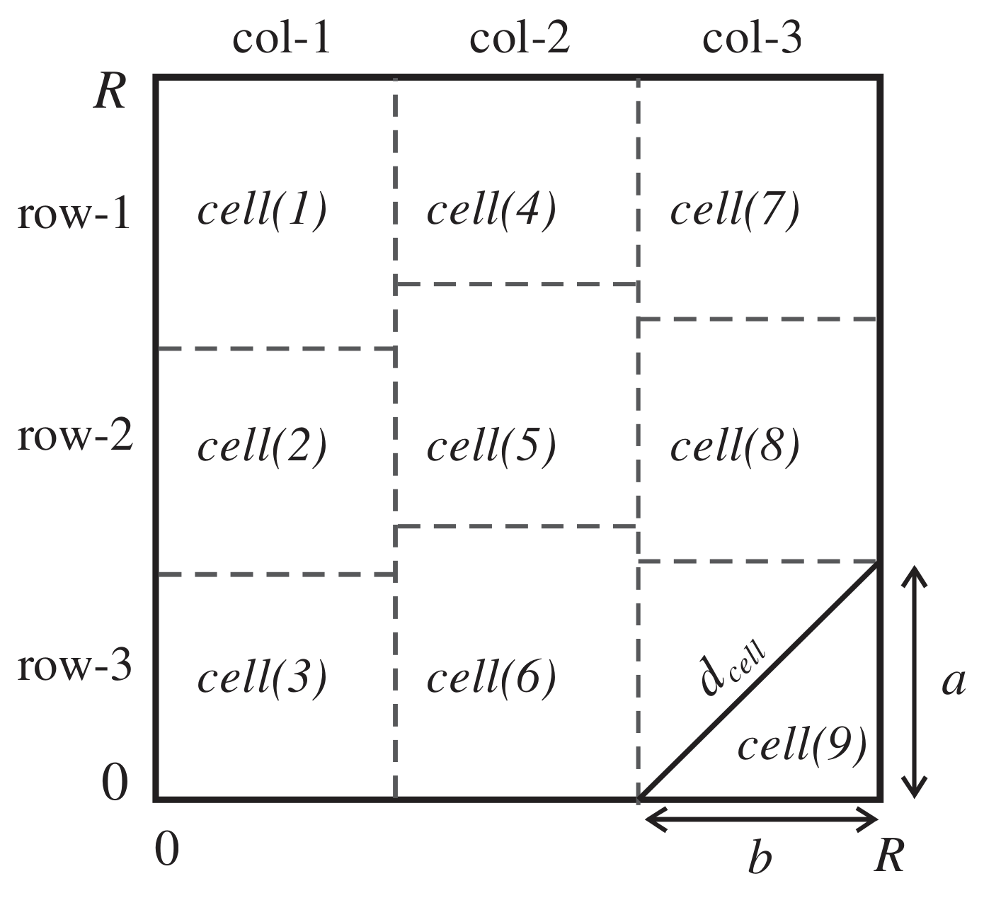
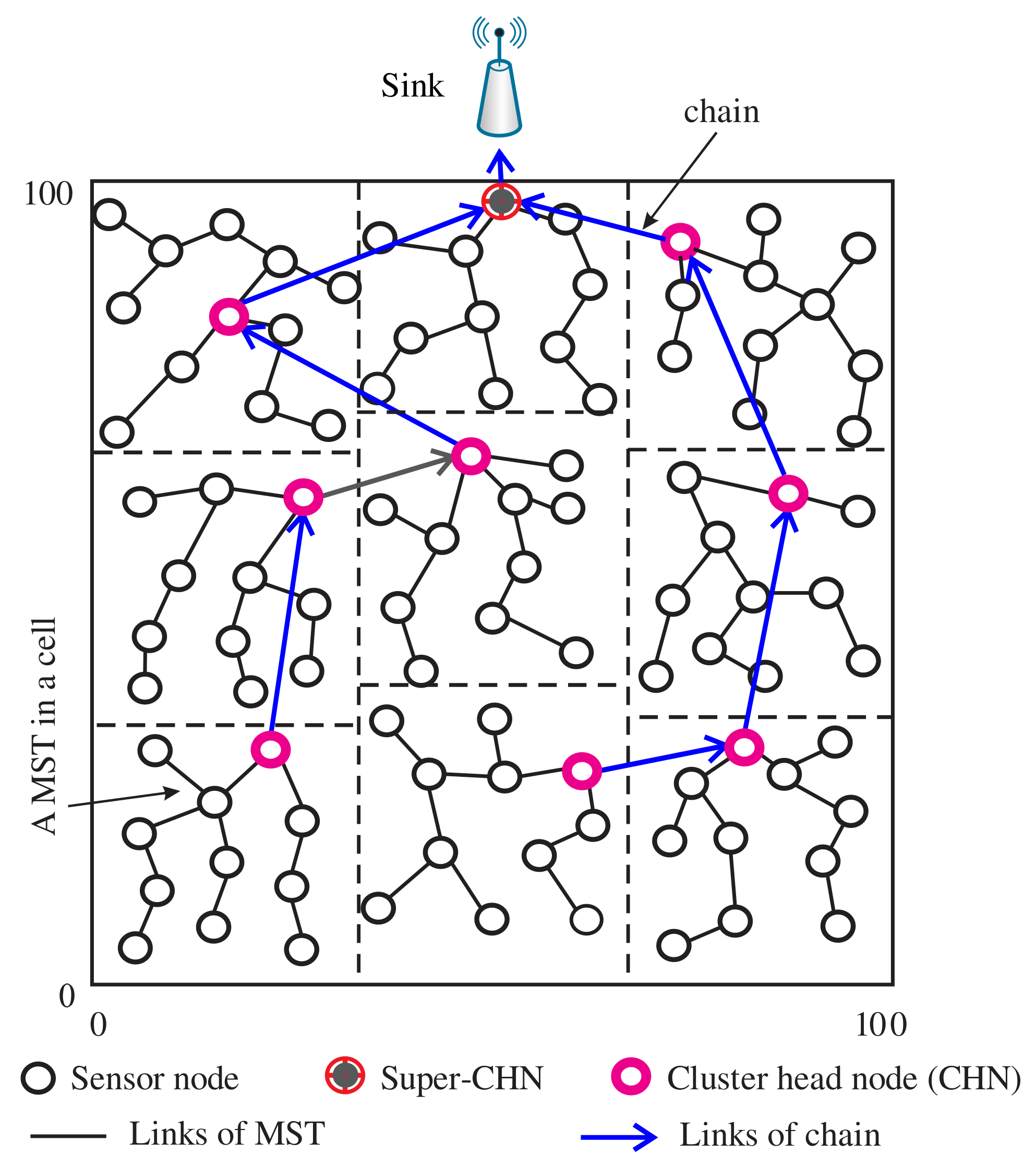
• We divide the whole monitored network region into the virtual grid with different cells (clusters) in order to guarantee a balanced number of live nodes jointly in each cell.
• We select CHN in each cell by considering the combination of the residual energy and the distance from the candidate CHN to the sink device.
• We combine tree and chain routing mechanisms for discovering data transmission routes from CMs to CHN and CHNs to the sink device by using the Kruskal algorithm and the ant colony algorithm to avoid the huge energy consumption made by the long distance between sensor nodes and the sink device.
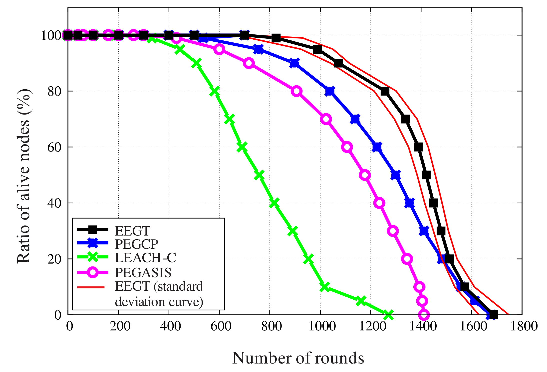
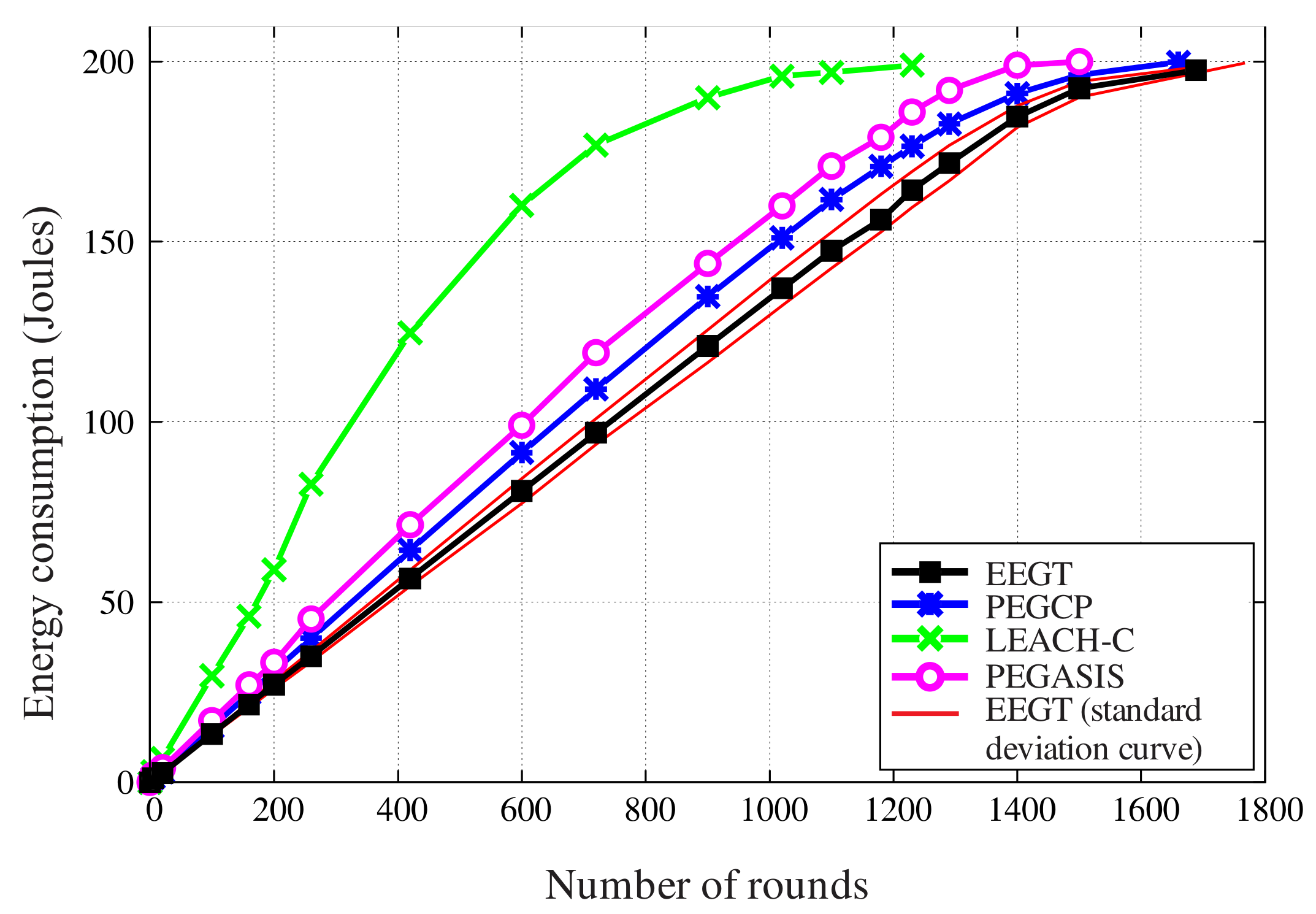
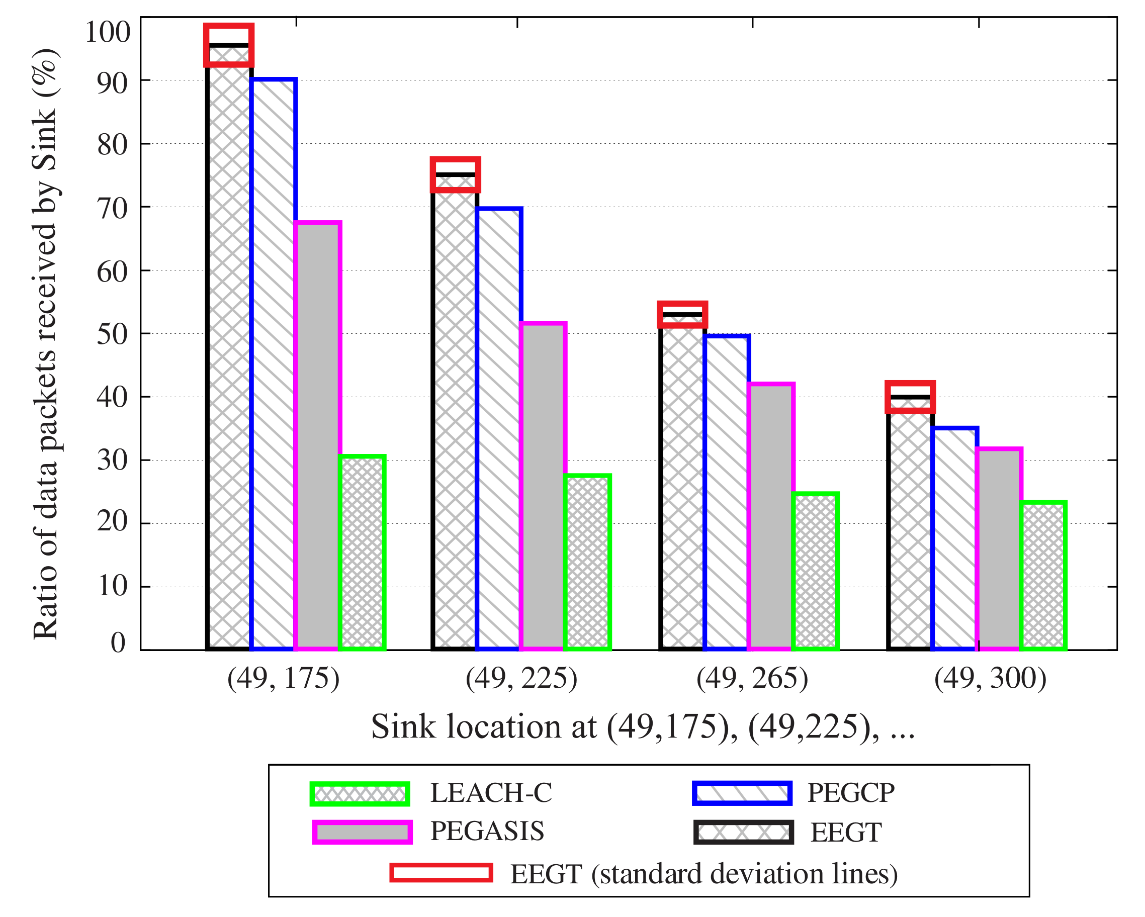
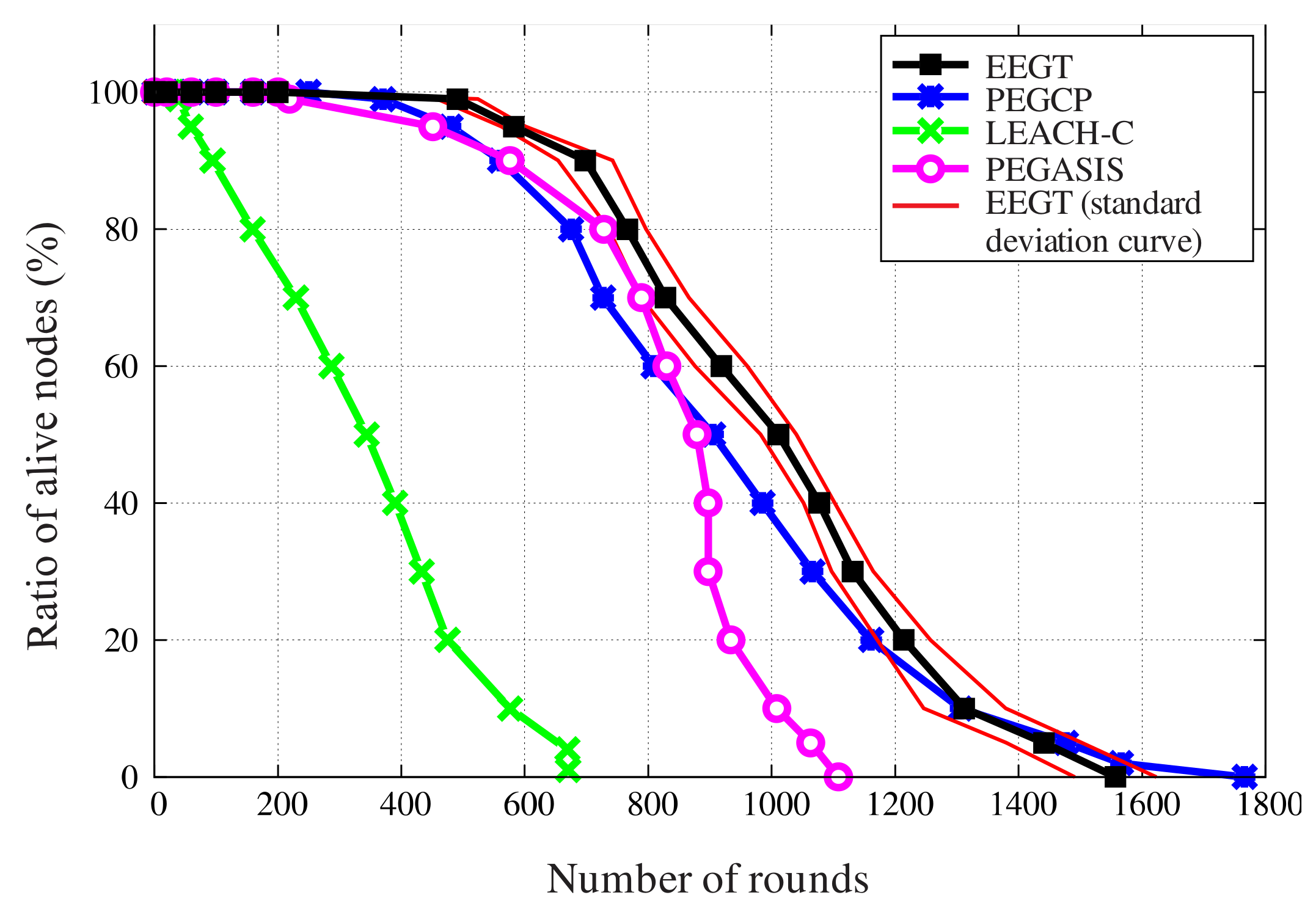
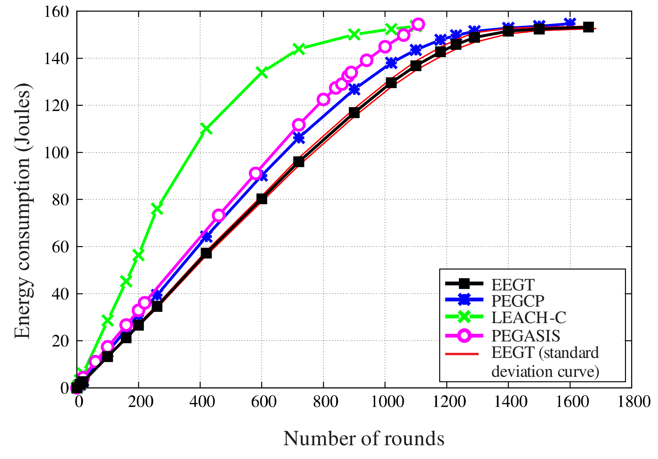
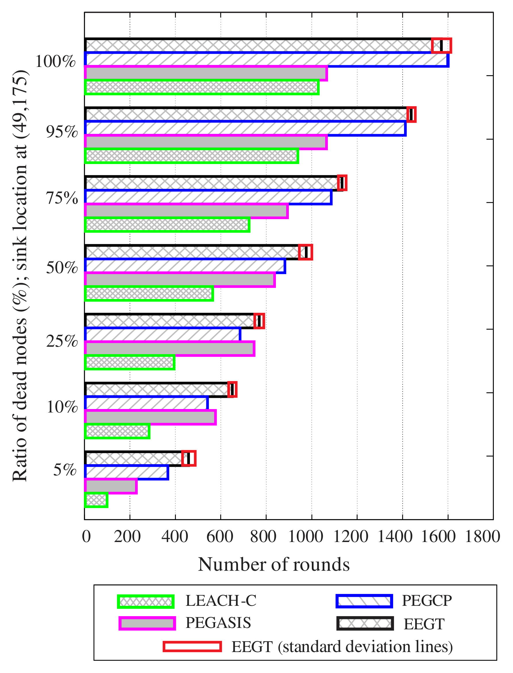
• In particular, we simulate the LEACH-C, PEGASIS, PEGCP, and EEGT routing protocols in many different scenarios. The simulation results in evidence that the network performance in terms of energy efficiency and the NL using our proposed protocol can be improved by 30%, 20%, and 10% compared with LEACH-C, PEGASIS, and PEGCP, respectively.

The remaining structure of this paper is organized as follows: Some previous related works are reviewed in Section 2. Section 3 presents the system models, and Section 4 describes the details of EEGT. In Section 5, the evaluation and analysis of simulation results are presented. Finally, Section 6 presents our conclusion.

2. Related Work

Many researchers have paid attention to how to reduce energy dissipation for IoT devices due to limited energy resources by the battery [26]. Anchitaalagammai et al. [27] have proposed efficient energy based on the clustering routing technique for resource management (EECBRM) in an IoT environment. Firstly, EECBRM employs the fuzzy logic method to group IoT devices (sensor nodes) in the network into clusters. Then, the optimal lion whale algorithm with tumbling (LWOT) is used to discover the optimal paths from IoT devices to the sink. Jaiswal and Anand [28] have proposed an energy efficiency optimal multi-path routing protocol to improve QoS in WSN for IoT applications (EOMR), in which the authors constructed multiple paths based on the estimated optimal factors with the measure of the lifespan of a node, reliability of communication, and traffic intensity. The authors in [29] have proposed an application-centric information-aware routing technique for the IoT platforms assisted by WSNs (ACIAR) by integrating WSN with IoT to find routes and process information for requested IoT applications. Shukla and Tripathi [30] introduced a scalable and energy-efficient routing protocol (SEEP) in which the total network area is divided into some sub-areas (clusters), and each cluster elects a cluster head (CH), a relay node (RN), and member nodes. RNs receive collected data packets from MNs and data fusion and send it to the CH. CHs are responsible for forwarding their fused data packet to another CH or the base station (BS). Rani et al. [31] proposed a dynamic clustering approach based on a genetic algorithm for WSN-based IoT applications. According to this proposal, the authors have established dynamic clustering in WSN by using parameters such as direct distance among nodes and the BS, communication energy cost, and the number of transmissions for the fitness function of heredity to decrease energy consumption. Lu et al. [32] presented a cluster tree-based energy-efficient routing protocol (CTEER) in WSNs. CTEER constructs a robust routing tree with a centered sink in which all sensor nodes can only communicate with their parent on the branches in the direction of the mobile sink in order to avoid lots of energy dissipation generated by long-distance communication. Therefore, it improves network efficiency. Lin et al.  [33] proposed an energy-efficient-adaptive clustering formation mechanism for WSN (ECFE) in which the CHs are chosen based on the value of energy efficiency welfare (EEW). EEW contains the residual energy of sensor nodes and the Euclidean distance among them in the same cluster. ECFE achieves energy-efficiency based on dividing the nodes into a grid topology. However, the data transmission between intra-grid and inter-grid nodes and the sink is the cause of much energy consumption in IoT applications. Tan et al. [34] proposed an energy-efficient distributed cluster-tree-based routing protocol for application IoT-based WSN, in which the clustering is completely distributed through exchanging messages at sensor nodes such as the LEACH protocol. The advantage of EE-DTC is that it combines the residual energy, the position, and the density of nodes as prime parameters for CH selection. Furthermore, EE-DTC discovers multi-hop routes for data transmission intra-clusters by building several MSTs to avoid communication over long links, thereby improving energy efficiency. However, distributed clustering increases extra energy consumption due to generating many messages overhead and increases workload at the CHs node due to constructing MSTs. Furthermore, using the single-hop communication method inter-cluster from CHNs towards the sink leads to high energy consumption.

3. System Model

In this section, we primarily introduce the network models and assumptions used in our proposal in heterogeneous and homogeneous WSNs.

3.1. Network Model

We use both homogeneous and heterogeneous WSN model that includes N smart sensor nodes randomly scattered in a region with $R\times R$ square meter size and a sink device. The sink device does not restrict energy, memory, and processing ability. In the homogeneous WSN model, all sensor devices are the same in proportions of initial energy level and other characteristics, but in heterogeneous WSNs, we assume that N sensing nodes are only different initial energy levels that are used with three kinds of sensor devices: $normal$, $advanced$, and $super$ sensors. Let $N_1$ and $N_2$ be the coefficient of N smart sensor nodes of $advanced$ and $super$ nodes that contain $\beta$ and $\alpha$ times greater energy levels than the $normal$ one, respectively.

$$\begin{array}{c}\hfill N_S=N\times N_1\times N_2,N_A=N\times N_1(1-N_2),\\ \hfill N_N=N(1-N_1),\mathrm{and}N=N_S+N_A+N_N\end{array}$$

(1)

where $N_S$, $N_A$ and $N_N$ are the respective quantity of $normal$, $advanced$, and $super$ sensor nodes [35,36]. If we assume $E_0$ denotes the initial energy level of each $normal$ sensor, then $E_0(1+\beta )$ and $E_0(1+\alpha )$ will be the initial energy of each $advanced$ and $super$ sensor node, respectively. Therefore, the total initial energy of WSN containing N sensor nodes is calculated as in Equation (2).

$$\begin{array}{cc}\hfill & E_{init}=E_0(N_N+N_A(1+\beta )+N_S(1+\alpha ))\hfill \end{array}$$

(2)

In general, if the N sensor nodes are distributed uniformly in the square region of $R\times R$ size, then the probability density function $\rho (x,y)$ can be computed as follows [21]:

$$\begin{array}{c}\hfill \rho (x,y)=1/R^2\end{array}$$

(3)

The average region size occupied by individual sensor nodes is indicated by Equation (4) [21]:

$$\begin{array}{c}\hfill A_{node}=R^2/N\end{array}$$

(4)

Let $N_{cell}$ be the number of grid cells (clusters) then the average region size of a cell is equivalent:

$$\begin{array}{c}\hfill A_{cell}=R^2/N_{cell}\end{array}$$

(5)

The average distance of a node to the nearest neighbor in each cell is

$$\begin{array}{c}\hfill d_{toNB}^2=R/\sqrt{N}\end{array}$$

(6)

Additionally, the longest distance from the CHN to the farthest node in each cell (as shown in Figure 5) is expressed in Equation (7):

$$\begin{array}{c}\hfill d_{max}=R/\sqrt{\pi N_{cell}}\end{array}$$

(7)

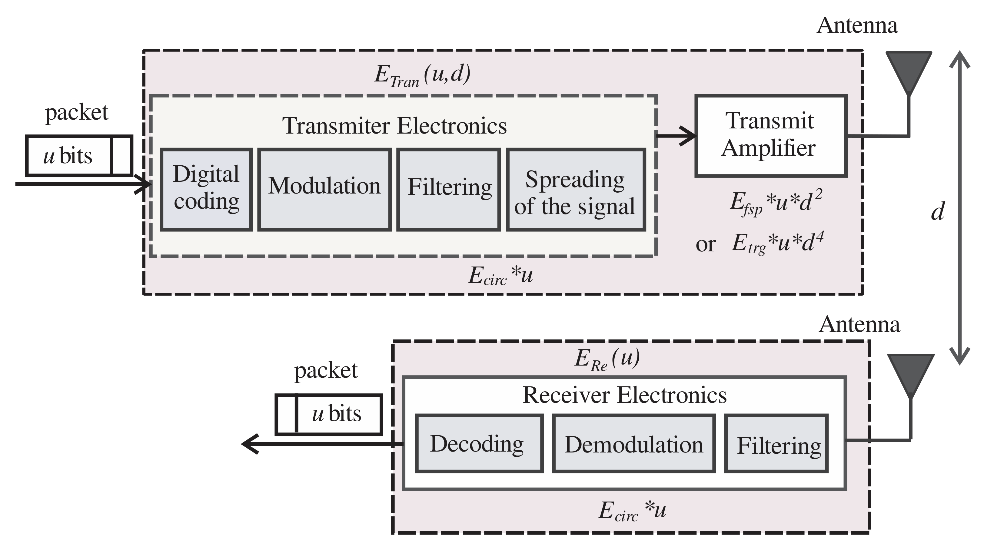
3.2. Energy Dissipation Model

Figure 2 illustrates the radio energy dissipation model in our proposal, which contains the transmitter component with the tasks such as digital coding, modulation, filtering, or spreading of the signal. In particular, the amplifying signal for transmission over long distances consumes more energy than the receiver, similar to the one discussed in [37].

Figure 2. Radio energy dissipation model.

According to this, whenever a sensing node transmits a packet with u bits data on the distance $d(x,y)$ from the sender x to the receiver y, either the free space propagation ($d^2$ energy loss) or two-ray ground reflection (multipath fading $d^4$ energy loss) model is used depending upon the distance $d(x,y)$. If the $d(x,y)$ value is greater or equal to the distance threshold $d_{cro}$, then the two-ray ground model is employed. Otherwise, the free space model will be employed, and that is given in Equation (8) [38].

$$E_{Tran}(u,d)=\left\{\begin{array}{cc}u(E_{circ}+E_{fsp}{d}^2)\hfill & ,\mathit{if}\mathit{d}<{\mathit{d}}_{\mathit{co}}\hfill \\ u(E_{circ}+E_{trg}{d}^4)\hfill & ,\mathit{if}\mathit{d}\ge {\mathit{d}}_{\mathit{co}}\hfill \end{array}\right.$$

(8)

where the fixed energy dissipation of the electronic transmitter or receiver circuits is $E_{circ}$ per bit, $E_{fsp}$ and $E_{trg}$ are the amplifier energy portion needed for a distance less than $d_{cro}$ and distance greater or equal $d_{cro}$, respectively. The distance threshold $d_{cro}$ is calculated in our simulation scenarios as Equation (9) [38].

$$d_{cro}=\sqrt{\frac{{\left(4\pi \right)}^{2}l{h}_t^2{h}_r^2}{{\lambda }^2}}=\sqrt{\frac{E_{fsp}}{E_{trg}}}$$

(9)

Moreover, the energy needed to receive the u bits of a packet data by the radio model can be indicated in Equation (10).

$$E_{Re}\left(u\right)=u{E}_{circ}$$

(10)

4. Proposed Protocol

This section describes our proposed EEGT protocol in detail, inspired by the LEACH-C protocol [21]. The operation of EEGT is separated into some rounds; each round consists of three periods: set-up period, path establishment period, and data transmission period. During the set-up period, the sink device divides the network region into logical grid cells that balance the number of sensors. Then the sink device chooses CHNs and super-CHN for grid cells based on the current energy level, the density of the node, and the Euclidean distance between nodes and the sink. In the path establishment period, the Kruskal and ant colony algorithm is combined to construct multi-hop data transmission routes to minimize energy consumption, an MST for intra-cells, and a chain for inter-cells toward the sink device. Finally, sensor nodes collect, aggregate data, and transmit them to the sink device. The overall operation of EEGT in a single round is shown in Figure 3.

Figure 3. Flowchart of the EEGT protocol in the operation of one round.

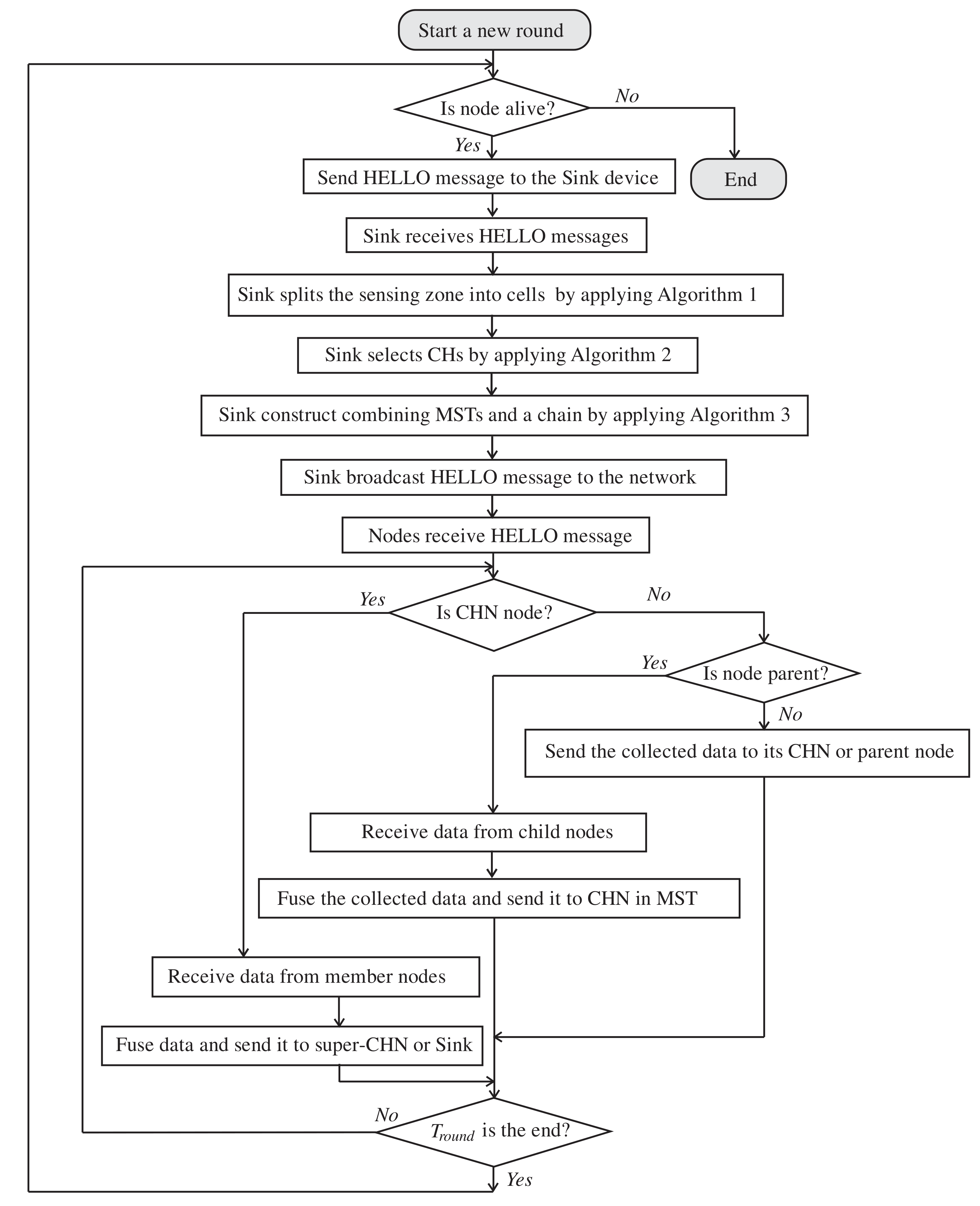
4.1. The Set-up Period

Step 1: Grid cell division of balancing the number of nodes

Firstly, BS receives messages HELLO which contains the current energy status and the location of all sensing nodes in the network transmitted to the sink device. Then, the sink divides the whole network sensing region into virtual grid cells that balance the number of sensing nodes, and each cell is considered a cluster. As shown in Figure 4, in which we assume a monitoring network region of $100\times 100$ square meters divided into nine grid cells with unequal rectangle sizes. Let $N_{row}$ and $N_{col}$ be the grid’s number of rows and columns, respectively. In the case of uniform distribution, node i-th can calculate the grid cell to which it belongs to the geographic coordinates (x, y) by using Equation (11).

$$\begin{array}{cc}\hfill cell\left(i\right)& =\left(idiv{N}_{row}\right)N_{row}+\left(imod{N}_{row}\right)\hfill \end{array}$$

(11)

$$\begin{array}{cc}\hfill d_{cell}& =\sqrt{a^2+b^2}\hfill \end{array}$$

(12)

where $d_{cell}$ indicates the diagonal of the grid cell; a and b are the length and width of one cell, respectively. The process of network area division into grid cells is illustrated in Algorithm 1 below:

Algorithm 1 Grid Division

Input: N sensor nodes with x, y positions, and current energy level Output: N sensors are distributed in logical $N_{cell}$ in a grid with $N/N_{cell}$ nodes for each cell. 1: Set N = The number of alive nodes in the network; 2: Sort N nodes non-decreasing according to the coordinates value x-axis; 3: Distribute balancing N nodes into $N_{column}$ as shown in Figure 5; 4: for each $col$ in {Number of columns} do 5:  Sort $N_{column}$ nodes non-decreasing according to the coordinates value y-axis; 6:  for each $col$ in {Number of columns} do 7:   Distribute balancing nodes $N_{column}$ into cells; 8:  end for 9: end for 10: Return {List of nodes in cells};

Figure 4. The energy efficiency of EEGT with different numbers of cells and the position of the sink device.

Figure 4 depicts the simulation results in the NS2 tool in comparison of the energy efficiency in kilobytes per joule and different numbers of cells; it is clear that EEGT is the most appropriate when the number of cells approximates about 4%, 5%, or 6% of the total of nodes. These values are also suitable with the optimum number of clusters, $k_{opt}$, which is indicated in Equation (13) [21].

$$\begin{array}{cc}\hfill & k_{opt}=\frac{\sqrt{N}}{2\pi }\sqrt{\frac{E_{fsp}}{E_{trg}}}\frac{R}{d_{toSink}^2}\hfill \end{array}$$

(13)

In addition, if the location of the sink device is nearer the network sensing region, the network performance achievement is better.

Step 2: CHNs selection

In the set-up period of each round, EEGT will select a CHN for each cell based on several criteria following:

• Average residual energy $\mathit{E}{\mathit{C}}_{\mathit{a}\mathit{v}\mathit{g}}\mathbf{(}\mathit{i}\mathbf{,}\mathit{j}\mathbf{)}$: $E{C}_{avg}(i,j)$ is the average current energy level of alive sensor nodes in cell i-th at round j-th (where i range from 1 to $N_{cell}$). This is the most important characteristic of candidate nodes to become CHN because of more energy consumed in transmitting to the sink device.

  $$\begin{array}{cc}\hfill & E{C}_{avg}(i,j)=\frac{1}{nc}\sum _{i=1}^{nc}{E}_i\left(r\right)\hfill \end{array}$$

  (14)

  where $nc$ and $E_{res}\left(t\right)$ are the number of nodes in cell i-th and the residual energy of sensor node $t$-th, respectively.
• Distance to BS (${\mathit{d}}_{\mathit{t}o\mathit{S}\mathit{i}\mathit{n}\mathit{k}}$): $d_{toSink}$ should be considered because according to Equation (8), the longer data transmission in the distance is, the more energy consumes (equal to the distance in the exponent of four). The Euclidean distance from the node i-th to the sink device is calculated below:

  $$\left|d_{toSink}\left(i,S\right)\right|=\sqrt{{\left(x_i-x_S\right)}^2+{\left(y_i-y_S\right)}^2}$$

  (15)

  where x and y and $x_{sink}$ and $y_{sink}$ are the coordinates of node i-th and the sink device, respectively.
• Intra and Inter cell distance ($\mathit{C}\mathit{D}\mathbf{\left(}\mathit{i}\mathbf{\right)}$): The objective of this criterion is to minimize intra-cell communication cost between MNs and respective CHN in an MST as well as minimize inter-cell communication cost from CHNs to the sink device in a chain that consumes less energy and balances the workload between CHNs. To achieve this objective, the $CD\left(i\right)$ is defined as the total geographic distance of the candidate CHNs within their cell, which is calculated as

  $$\begin{array}{c}\hfill CD\left(i\right)=\frac{h{\sum }_{j=1}^{nc}d(i,j)}{mi{n}_{j\in SN\left(i\right)}\left(d(i,j)\right)}\end{array}$$

  (16)

  where h and $SN\left(i\right)$ are the numbers of neighbor nodes and set of neighbor nodes of the candidate node i-th, respectively.
• Cost function: All the appropriate parameters introduced are combined in order to select suitable CHN for each cell, whose residual energy is higher than $E{C}_{avg}(i,j)$ and has a maximum cost function value as Equation (17) follows:

  $$\begin{array}{c}\hfill cost\left(i\right)=\left(c_1{E}_{res}\left(i\right)\right)\times \left(c_{2}CD\left(i\right)\right)\times \frac{c_3}{d_{toSink}(i,S)}\end{array}$$

  (17)
  The user establishes the coefficient parameters within cost function $c_j$ $(j=1,2,3)$ for the heterogeneous and homogeneous network.

Step 3: Super-CHN selection

In EEGT, only several super-CHNs are responsible for forwarding aggregated data packets to the sink to preserve energy in other nodes, so the distance from them to the sink device is as short as possible. In addition, the higher the residual energy of the candidate super-CHN is, the better the energy efficiency of the network achieves. Therefore, if the distance from the candidate super-CHN to the sink device is smaller than that of the average distance $DC{H}_{avg}$ between CHNs within the list of CHNs to the sink device or if its position is in the “row-1” region (Figure 5). If it has the highest P values, then CHN will be selected as super-CH in the current round. The $DC{H}_{avg}$ and P can be calculated as Equations (18) and (19) follow:

$$\begin{array}{c}\hfill DC{H}_{avg}=\frac{1}{N_{cell}}\sum _{i=1}^{N_{cell}}d(C{H}_i,Sink)\end{array}$$

(18)

$$\begin{array}{c}\hfill P\left(i\right)=\frac{c_4{E}_{res}\left(i\right)}{d_{toSink}(i,S)}\end{array}$$

(19)

where $P\left(i\right)$ represents the ratio between the remaining energy of sensor node i-th and the distance from sensor node i-th to the sink. The process of cell head selection is illustrated in Algorithm 2 below:

Figure 5. An example of network topology partitioned into logical grid cells.

Algorithm 2 Cell Head Selection

Input: $N_{cell}$ number of cells, N sensors distributed in $N_{cell}$ cells, and their position of them Output: List of CHNs in each cell and one or more super-CHNs. 1: fori = 1 to $N_{cell}$ do 2:  Compute the residual average energy of nodes in each cell as in Equation (14) 3:  Select CHN for cell i-th, which has a maximum cost function value as Equation (17) 4:  Append CHN to List of the CHNs 5: end for 6: $minD$ = Maximum value; 7: for each CH in {List of the CHNs} do 8:  $disSink$ ← Compute the average distance from CHNs to the sink as Equation (18) 9:  $P_i$ = Compute the parameter criterion P as Equation (19); 10:  if ($disSink$ < $minD$) and ($P_i$ is the highest) then 11:   $minD$ = $disSink$; 12:   $super-CH$ = $CH{N}_i$; 13:  end if 14: end for 15: return: {List of the CHNs and super-CHNs};

4.2. MST and Chain Construction Period

In this period, all nodes in each cell are organized into one MST with a CHN as a root inspiration of the Kruskal algorithm. To finish this work, we assume that nodes in a cell of WSN are considered as an undirected graph G (V, E, D) completely, where V indicates a set of distributed sensing nodes, E denotes a set of communication links connected by the sensor nodes, and D represents the set of distance values on E, respectively. Furthermore, in order to decrease energy consumption in forwarding sensed data packets to the sink device, CHNs will find the shortest path from them to super-CHNs; this makes the chain approach based on the ant colony algorithm by calculating the transition probability value to select the next CHN on the path towards the sink [39,40]. Assuming that the ant a-th is at cell i-th with CHN i-th and it tends to move to the cell destination, which contains super-CHN, it will randomly select cell j-th (containing CHN j-th) with the transition probability on the path $p_{ij}^a$ that can be computed as Equation (20) below:

$$P_{ij}^a=\left\{\begin{array}{cc}\frac{{\left[T_{ij\left(t\right)}\right]}^{\alpha }\times {\left[\frac{1}{d_{toCH}(i,j)}\right]}^{\beta }}{{\sum }_{l\in S_k\left(i\right)}{\left[T_{il}\right]}^{\alpha }{\left[\frac{1}{d_{toCH}(i,l)}\right]}^{\beta }}\hfill & ,\mathrm{if}\mathrm{j}\in S_k\left(i\right)\hfill \\ 0\hfill & ,\mathrm{otherwise}\hfill \end{array}\right.$$

(20)

where $T_{ij}$ is the amount of pheromone which expresses the current energy level of the CHN j-th at time t, $d_{toCH}(i,j)$ indicates the distance between CHN i-th and CHN j-th, $S_k\left(i\right)$ is the set of direct neighbors of CHN i-th where ant a-th can move to, $\alpha$ and $\beta$ are parameters that can be used to control the residual energy level and the distance d to CHN j-th ($\alpha$, $\beta$ > 0), respectively. In reality, the more ants that go along a path during the unit time, the more pheromone convenes along the path. However, at the same time, the pheromone on the path is also easily volatile; hence, to update the amount of pheromone $T_{ij}$ at the next time on the selected path to super-CHN, CHN i-th updates the pheromone level according to Equation (21) below:

$$\begin{array}{c}\hfill T_{ij}(t+1)=(1-\varphi )T_{ij}+T_{ij}(t+1)=(1-\varphi )T_{ij}+\sum _{l=1}^{N_{row}}▵T_{ij}^l\left(t\right)\end{array}$$

(21)

where $\varphi$ denotes the volatile factor of pheromone $(0<\varphi <1)$, and $▵T_{ij}^l\left(t\right)$ represents the addition of the pheromone on path j-th selected by ant a-th after one iteration. If the ant a-th goes over the CHN j-th, then $▵T_{ij}^l\left(t\right)$ will be equal $1/L\left(t\right)$, where L is the optimal path length and zero otherwise. The process of building the MST and chain is illustrated in Algorithm 3 below:

Algorithm 3 MSTs and Chain Formation

Input: List of the sensor nodes in cells, CH, super-CH Output: - MSTs for cells with CH as a root                - A chain connected CHNs and the sink device. 1: Set MSTs = ⊘; 2: for $i=1$ to $N_{cell}$ do 3:  Set count = 0; 4:  Set ei = 1; 5:  Set TREEi = TREEi ∪ {CHNi}; 6:  Set CHNi as the root node; 7:  for i = 1 to {The number of edges in cell(i)} do 8:   E[i].chosen = FALSE; 9:  end for 10:  Sort {list of edges in set E} as not ascending of distance values 11:  while (ei < {the number of edges in E} − 1) do 12:   Select edge ei in E, whose E[ei].chosen is FALSE; 13:   Set u = get root of edge (E[ei].u); 14:   Set v = get root of edge (E[ei].v); 15:   if (u and v are on two different trees) then 16:    Union(E[ei].u,E[ei].v) 17:    E[i].chosen = TRUE; 18:    Set count = count + 1; 19:    if (count = {number of nodes in cell(i)} − 1) then 20:     break; 21:    end if 22:   end if 23:   Set ei = ei + 1; 24:  end while 25:  for each edge i in {List of the edges in E} do 26:   if (E[i].mark = TRUE) then 27:    TREEi = TREEi ∪ {E[i].u, E[i].v}; 28:   end if 29:  end for 30:  Set MSTS = MSTs ∪ TREEi; 31: end for 32: Set CHAIN = {super-CH}; 33: Set super-CH as root device; 34: for CHNi = 1 to {The number of CHNs} do 35:  Find the path from CHNi to CHNj by calculating the transition probability value 36:  as Equation (20); 37:  Update the pheromone according to Equation (21) 38:  Connect CHNi and CHNj into CHAIN 39:  Discard the CHNi in {List of the CHN devices} 40: end for 41: Create slots time as TDMA schedule for all nodes to communicate in cells; 42: Create CDMA codes for CHNs to forward data along CHAIN to the sink device; 43: Broadcast the TDMA schedule, CDMA code, MSTs, and CHAIN to the network; 44: return {MSTs and CHAIN};

Figure 6 illustrates an example of clustering, CHN selection, and data transmission route establishment, which includes 100 sensing nodes and the sink device deployed in the region of 100 × 100 m${}^2$.

Figure 6. The network topology with EEGT protocol in one round.

4.3. Data Transmission Stage

After finishing the CHN selection and establishing the multi-hop routes above, sensor nodes monitor the environment and periodically transmit sensed data packets to the sink through trees and a chain with intra-cell and inter-cell communication, respectively. Firstly, the farthest nodes in each MST will start sending to their parent node toward their CHN. The parent nodes receive the data packets, aggregate them, compress them with their own sensed data in a single packet, and transmit them to the upper-level nodes in the MST. The CHNs send to the next nodes along the chain to super-CHN. Whenever the super-CH nodes receive all the data, they will forward the data packets to the sink device after it is aggregated in the same way. After an interval of time, the next round will be started again by rebuilding the grid with several cells (clusters), reelecting CHNs and super-CHN, and reconstructing the tree and chain in the network for a new round.

5. Simulation and Performance Evaluation

5.1. Simulation Parameters

To analyze EEGT performance, we simulated EEGT, LEACH-C [21], PEGASIS [22], and PEGCP [25] by network simulator ns-2 (v.2.34) [41,42] installed in the Ubuntu 12.04 virtual machine using the scenarios with the $c_1=0.5$, $c_2=500$ m, $c_3=0.05$ m, and other parameters that are described in Table 1 [21,36,43].

Table 1. The simulation parameters.

No. Item	Parameters Description	Value
1	Simulation region	100 m × 100 m
2	Number of sensing nodes	100 nodes
3	$E_{circ}$ (Radio electric circuit energy right)	50 nJ/bit
4	$E_{trg}$ (Radio two-ray ground energy right)	100 pJ/bit/m${}^2$
5	$E_{fsp}$ (Radio free space energy)	0.013 pJ/bit/m${}^4$
6	$E_{DF}$ (Data fusion energy)	5 nJ/bit
7	Packet size	1024 bytes
8	Simulation time	3600 s
9	The locations of the sink	(49,175); (49,225); (49,300)
For homogeneous network model
10	$E_0$ (Initial energy of node)	2 J
For heterogeneous network model
11	$E_0$ (Initial energy of node)	1 J
12	$N_1$	0.5
13	$N_2$	0.4
14	$\alpha$	0.5
15	$\beta$	2

5.2. Simulation Scenario

In this experiment, we have simulated the LEACH-C [21], PEGASIS [22], PEGCP [25], and EEGT protocols in many different scenarios to advance the reliability of the protocols in practice. Specifically, we employed the “./setdest -v 1 -n 100 -t 1 -x 100 -y 100 -M 1 >sceni.txt” command in ns2 to create randomly many different scenarios with the same simulation parameters. In order to determine how many scenarios ($nscen$) are needed to run in simulation, we perform some steps as follows:

Step 1: 

Generate randomly 50 times for 50 different scenarios with the number of sensor nodes $N=100$ nodes in 100 × 100 m${}^2$ simulation area; in these 50 scenarios we remove the movement partly because we assume the sensor network is the stationary state after deployment.

Step 2: 

Run a simulation of LEACH-C, PEGASIS, PEGCP, and EEGT protocols on the first scenario ($i=1$). The simulation results are represented in the table, which indicates the proportion of alive nodes, total energy consumed, and rate of data packets received by the BS.

Step 3: 

Select performance metrics; here, we choose the energy efficiency and network lifespan metrics to evaluate.

Step 4: 

Run the next scenario ($i=i+1$); we present the simulation results in the table that shows the percentage of the dead nodes, total energy consumed, and amount of data packets obtained by the sink.

Step 5: 

Calculate the medium $m{e}_x$, standard deviation $\delta$, and standard deviation ratio $\chi$ value according to Equations (22)–(24) on the table of the simulation results.

Step 6: 

Compare the obtained results with previous ones. If the ratio of standard deviation is less than $\chi \%$, then stop the simulation and go to Step 7, because if we run more simulations, the standard deviation ratio ($\chi$) will not change. Otherwise, go to Step 4.

Step 7: 

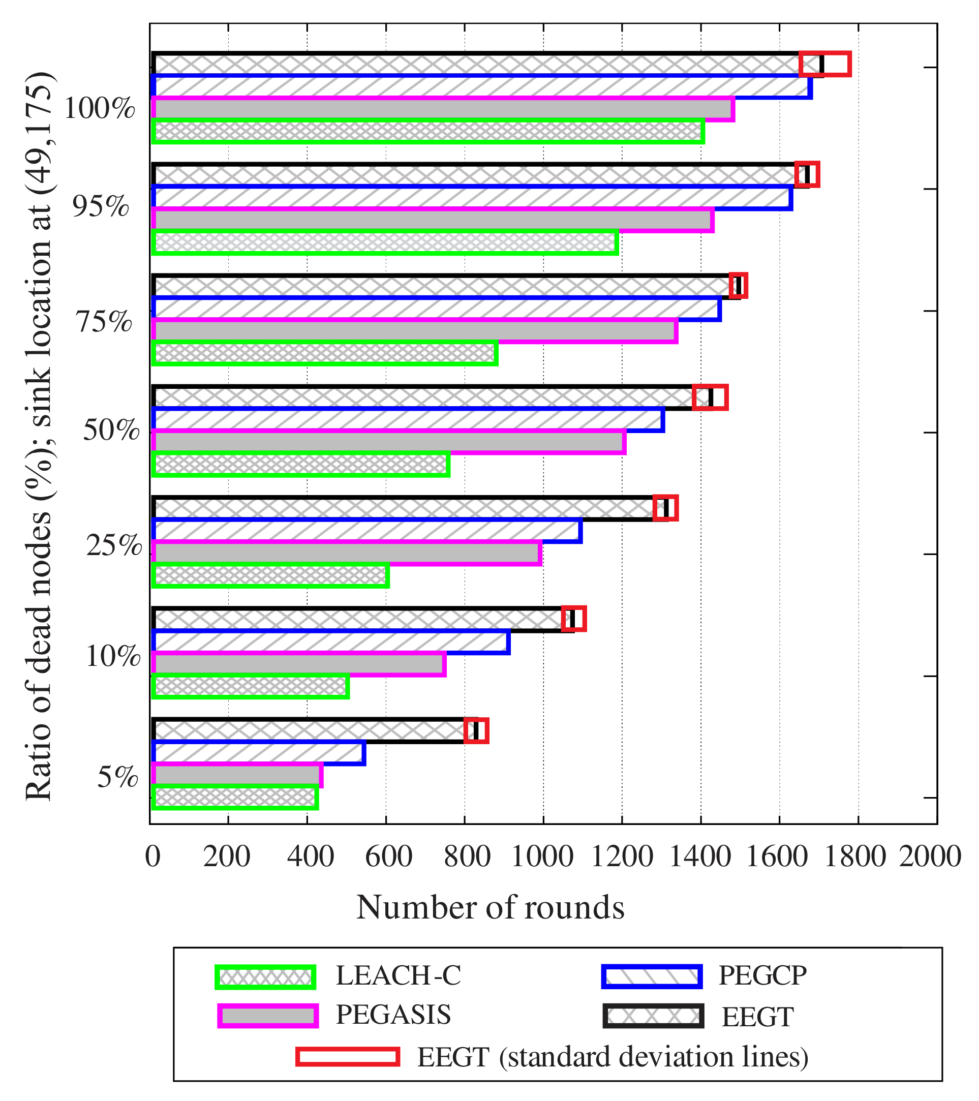
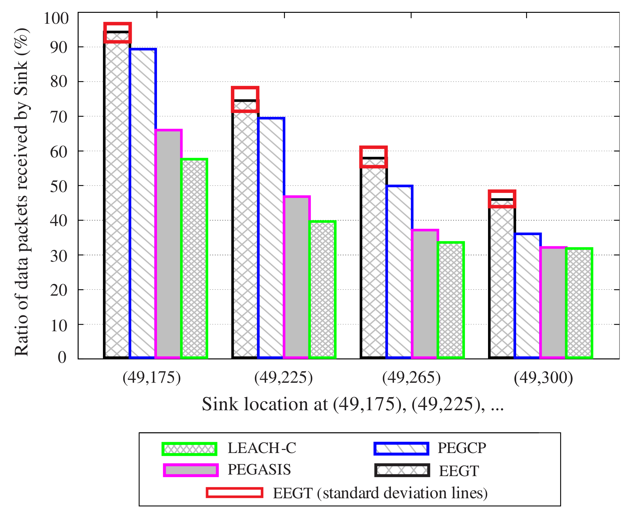
Graph the simulation results based on the table medium. The rate of standard deviation with the scenario $nscen=i$ to analyze LEACH-C, PEGASIS, PEGCP, and EEGT protocol performance in terms of the percentage of alive nodes, energy consumption, and the number of data packets received by the sink with the different location according to NL.

We assume the mean $m{e}_i$, standard deviation $\delta$, and standard deviation ratio $\chi$ can be calculated as in the equations below:

$$\begin{array}{cc}\hfill & m{e}_i=\frac{1}{nscen}\sum _{i=1}^{nscen}sce{n}_i\hfill \end{array}$$

(22)

$$\begin{array}{cc}\hfill & {\sigma }_i=\sqrt{\frac{1}{nscen}\sum _{i=1}^{nscen}(m{e}_i-sce{n}_i)}\hfill \end{array}$$

(23)

$$\begin{array}{cc}\hfill & \chi ={\sigma }_i/max\left(sce{n}_i\right)\mathrm{with}i=1\mathrm{to}nscen\hfill \end{array}$$

(24)

where $sce{n}_i$ is the simulation results of i-th scenario with LEACH-C, PEGASIS, PEGCP, and EEGT protocols. Specifically, we also run the simulation in many different scenarios for homogeneous and heterogeneous networks with the parameters given in Table 1.

5.3. Simulation Results and Analysis

5.3.1. Homogeneous Network Model

Figure 7 shows that the ratio of still-alive sensor nodes in the network (y-axis) per network lifespan depicted the number of rounds (x-axis) in LEACH-C, PEGASIS, PEGCP, and EEGT protocols with the location of the sink device at (49, 175). The red lines represent the standard deviation of the ratio of the medium ($m{e}_x$) of EEGT protocol, with $\chi$ deviation ratio equal to 3.9% corresponding to the number of different scenarios $nscen=20$. This means that if we run more simulation scenarios, the achievement results cannot also be outside of the standard deviation curve; we get the value of $\chi$ deviation ratio with LEACH-C 6.8% ($nscen=17$), PEGASIS 5.6% ($nscen=19$), PEGCP of 5.4% ($nscen=20$) at the time the network has 99% of the node death. Due to the rotation of CH role and selection of CHNs based on the suitable criteria parameters, the proposed protocol obtains a better balance of energy consumption than the three existing protocols and, as a result, extends the NL.

Figure 7. The ratio of the number of alive sensors per network lifespan (rounds) in the homogeneous network.

In Figure 8, the total energy drained by all nodes of four protocols is shown during each round. From these simulation results, we can see that EEGT consumes less energy than the three other protocols because EEGT avoids communication over long distances by establishing multi-hop data transmission routes intra-cellularly and inter-cellularly. Furthermore, in LEACH-C, PEGASIS, and PEGCP, most of the CHNs transmit data packets directly to the base station. Meanwhile, EEGT only allows super-CHs nodes to forward data packets to the sink device with a “short-link” and the other nodes will transmit the fused data packets in the path base on the ant algorithm. So, EEGT achieves better energy efficiency and improves the network lifespan compared to LEACH-C, PEGASIS, and PEGCP.

Figure 8. Total energy consumption by sensors in a homogeneous network.

Figure 9 shows the ratio of dead nodes according to the network lifespan (rounds), in which the LEACH-C and PEGASIS have a ratio of 5% dead nodes at approximately the 410th and 420th round and stop working at the 1400th and 1440th round, respectively. Meanwhile, the PEGCP and EEGT protocols work with 95% of the nodes alive to the 550th and 800th round and stop working at the 1680th and 1700th round, respectively.

Figure 9. The ratio of dead sensors per network lifespan (rounds) in a homogeneous network.

Figure 10 illustrates the ratio of data packets that were successfully delivered to the sink device at the end of the simulation of 20 different scenarios with EEGT, the average of the standard deviation ratio $\chi$ = 3.1% indicated by the red lines when the location of the sink device is being changed. The three other LEACH-C, PEGASIS, and PEGCP protocols achieve the average standard deviation ratio of $\chi =3.6$% of 18 different scenarios, $\chi =4.2$% of 18 different scenarios, and $\chi =3.0$% of 17 different scenarios, respectively. There is a stable decline in the number of data packets the sink device receives when we move it from the initial point (49, 175) to the farthest point (49, 300) in the simulation area. However, the ratio of the number of data packets received by the sink device of our proposed protocol is improved by approximately 40%, 20%, and 15% compared with LEACH-C, PEGASIS, and PEGCP protocols, respectively. This is because EEGT achieved the balance of energy consumption among sensor nodes in the network; the more balanced the energy consumption, the greater the energy efficiency.

Figure 10. The ratio of data packets received at the sink device with different locations in a homogeneous network.

Furthermore, Table 2 presents the simulation results in terms of the percentage of dead nodes and energy efficiency (EE) with the size of different rounds ($t_{round}$) from 10 to 700 s for WSNs in a homogeneous model. After we process the simulation from Step 2 to Step 7 as in Section 5.2, we have selected the medium value and standard deviation ratio after running 20 different scenarios applied with EEGT protocol ($t_{round}=10$, EE = 1041 (Kbytes/Joule), $\chi =1.0$%, and 1% dead node = 829th round); with the LEACH-C protocol, the number of processed different scenarios is $nscen=19$, and ($t_{round}$ = 10, EE = 610 (Kbytes/Joule), $\chi$ = 2.5%, and 1% dead node = 478th round); with the PEGASIS protocol, the number of processed different scenarios is $nscen=20$, and ($t_{round}$ = 10, EE = 657 (Kbytes/Joule), $\chi =2.5$%, and 1% dead node = 631st round); and with the PEGCP protocol, the number of executed different scenarios is $nscen=20$, and ($t_{round}=20$, EE = 1020 (Kbytes/Joule), $\chi =7.6$%, and 1% dead node = 539th round). Normally, if $t_{round}$ increases, throughput and energy efficiency will also increase, but the 1% dead node will be earlier in all four protocols. However, for the LEACH-C protocol, when $t_{round}=300$, EE = 120 (Kbytes/Joule), CHNs die too early, so the collected information of the whole cluster is not sent to the sink device. In most cases, our proposed EEGT protocol still achieves better energy efficiency than the three conventional protocols in changing the size of rounds, and the most suitable of our proposal EEGT is EE = 1108 (Kbytes/Joule) and 1% dead node = 877th round when $t_{round}=50$ s.

Table 2. The comparative energy efficiency of EEGT to other protocols with different $t_{round}$ values in homogeneous WSN.

			The Percentage of Dead Nodes
Protocols	Rounds	EE (Kbytes/Joule)	1%	10%	25%	50%	75%	95%	100%
	(s)	$(\mathit{\chi }\%)$	$(\mathit{\chi }\%)$	$(\mathit{\chi }\%)$	$(\mathit{\chi }\%)$	$(\mathit{\chi }\%)$	$(\mathit{\chi }\%)$	$(\mathit{\chi }\%)$	$(\mathit{\chi }\%)$
	10	610(2.5)	478(14.3)	603(12.3)	685(2.9)	762(2.9)	857(2.6)	988(5)	1140(7.8)
	50	720(2.5)	34(14.4)	178(21.4)	442(9.7)	857(5.2)	1166(3.2)	1600(5.6)	1709.5(4.7)
LEACH-C,	100	1050(12)	32(13.1)	172(21.8)	547(27.5)	1260(17.7)	2141(12)	2530(13)	2630(9.9)
[21]	300	120(4.3)	32(16.2)	506(21.1)	2023(22.2)	2610(6.8)	2886(3.9)	3074(3.5)	3178(2.5)
	10	657(2.5)	631(15.3)	816(5.8)	947(3.5)	999(21.9)	1116(3.0)	1230(2.3)	1247(2.5)
	50	889(1.9)	62(53.5)	485(16.4)	1200(5.1)	1569(1.5)	1658(1.4)	1680(1.2)	1711(1.3)
PEGASIS,	100	1009(2.7)	49(18.4)	926(0.8)	1715(0.9)	1811(0.6)	1865(1.7)	1896(0.4)	1974(3)
[22]	300	1051(6.6)	50(20.3)	50(20.3)	1712(12.3)	1941(2.1)	2001(1.5)	2029(1.7)	2155(3.9)
	20	1020(7.6)	539(11.3)	905(5.4)	1087(4.3)	1030(3.1)	1450(4.0)	1617(4.8)	1658(6)
	50	1071(1.2)	520(19.0)	920(7.6)	1125(5.3)	1353(3.4)	1529(4.6)	1685(4.2)	1715(4.1)
PEGCP,	100	1095(1.5)	404(32.5)	899(6.9)	1137(7.7)	1372(5.6)	1549(4.7)	1781(5.2)	1805(4.9)
[25]	300	1183(1.1)	231(15.9)	827(5.3)	1127(4)	1433(2.6)	1674(4.9)	1923(5.5)	2056(4.6)
	500	1251(1.6)	233(15.3)	808(13.6)	1164(5)	1456(2.8)	1752(4.1)	2017(5.7)	2166(2.3)
	10	1041(1.0)	829(15)	1065(4.8)	1297(6.5)	1395(7.4)	1491(2.8)	1640(5.0)	1663(3.8)
	50	1108(1.2)	877(17)	1105(2)	1351(3.7)	1484(1.7)	1564(2.2)	1724(2.9)	1756(2.6)
EEGT	100	1143(30.3)	861(13.4)	1107(0.6)	1300(1.5)	1503(0.8)	1610(0.6)	1836(1.7)	1860(1.3)
	300	1234(23.2)	519(36.4)	1081(22.7)	1257(22.9))	1572(22.4)	1710(22.5)	1999(23.3)	2120(22.5)
	500	1278(1.5)	404(30.8)	1061(7.3)	1306(5.9)	1620(0.8)	1892(3.1)	2240(2.9)	2180(13.1)

5.3.2. Heterogeneous Network Model

In this research, we have implemented a 50% $normal$ node, 30% $advanced$ node, and 20% $super$ node for a heterogeneous network model. The energy level of the $advanced$ node and the $super$ node is initialed 1.5 and 3 times greater than the $normal$ node (initial energy of $normal$ node $E_0$ = 1 Joule), respectively. As presented in Equation (1), we establish the total energy initial $E_{init}$ =155 Joules for all nodes, in which $NN=50$$normal$ sensor nodes; $NA=30$$advanced$ nodes; and $NS=20$$super$ nodes. The simulation parameters are configured for discussed all protocols, as shown in Table 1. In order to evaluate the performance of EEGT, we also perform the simulation from Step 2 to Step 7 as in Section 5.2; the simulation results are graphed in the figures following after we calculated the medium value and standard deviation ratio.

As shown in Figure 11, we can see that the ratio of alive nodes decreases along the network lifespan (number of rounds) in the heterogeneous network. By considering the residual energy factor of the nodes in the CHNs decision, the EEGT improves the performance of the network compared with LEACH-C, PEGASIS, and PEGCP in terms of energy consumption balance and the 1% node death even though the PEGCP achieves the last node death longer than three others protocols due to unbalanced energy consumption.

Figure 11. The ratio of the number of alive sensors per round in heterogeneous network.

Figure 12 depicts the total energy consumption of smart micro-sensor nodes in Joules during the network lifespan (rounds) in a heterogeneous network with four protocols. Based on the simulation results, we obtain the value at that time of the standard deviation ratio $\chi$ = 4.9%; $nscen=19$ different scenarios with LEACH-C; $\chi =4.1$%, $nscen=19$ different scenarios with PEGASIS; $\chi$ = 2.3%; $nscen=19$ different scenarios with PEGCP; and $\chi =2.8$%, $nscen=19$ different scenarios with EEGT protocols. As shown in Figure 12, it is evident that the energy consumption of the network increases drastically when the network lifespan increases. However, our proposed EEGT protocol has the lowest energy consumption compared with the other three popular protocols due to reducing communication distance in the data transmission routes to the sink device.

Figure 12. Total energy consumption by sensors in a heterogeneous network.

Figure 13 is a reverse representation of Figure 10 about the percentage of dead nodes in the heterogeneous network, which shows 5%, 10%, 25%, 50%, 75%, 95%, and 100% node death. The EEGT protocol improved the network lifespan by decreasing the ratio of dead nodes from 5% to 95% in comparison with the existing protocols such as LEACH-C, PEGASIS, and PEGCP. However, PEGCP has a longer network lifespan at 100% node death because PEGCP unbalances energy consumption among nodes in the network.

Figure 13. The ratio of dead sensors per network lifespan (rounds) in a heterogeneous network.

Figure 14 presents the ratio of data packets the sink device receives when its location is varied. This is also an important performance measurement for estimating the energy efficiency utilization of routing protocols because the more efficiently it uses in the network, the more data packets are received in the sink device. The ratio of the data packet received by EEGT attained about 95% with the average of the standard deviation ratio obtaining $\chi$ by approximately 3.0% in the 19 different scenarios, which are also higher than those of LEACH-C, PEGASIS, and PEGCP, with about 30% with $\chi$ by approximately 1.9% in 17 different scenarios; 20% with $\chi$ by approximate 4.6% in 18 different scenarios; and 5% with $\chi$ by approximately 1.8% in 19 different scenarios, respectively. This is because our proposed protocol can calculate suitable time duration during the steady data transmission phase for each round so that the EEGT protocol achieves greater energy efficiency and longer network lifespan in both heterogeneous and homogeneous network models.

Figure 14. The ratio of data packets received at the sink device with different locations of it in a heterogeneous network.

Furthermore, Table 3 presents the energy efficiency and the percentage of dead nodes in the FDD, HDD, and LDD for LEACH-C, PEGASIS, PEGCP, and EEGT with changing $t_{round}$ from 10 to 700 s of the heterogeneous network model. We can see in Table 3 that the EEGT protocol achieves better energy efficiency than that of the three existing protocols because the energy consumed for data transmission paths based on MST and chain is lower than in a single hop due to the distances among connected nodes being smaller. Specifically, the energy efficiency of our proposed EEGT protocol at $t_{round}$ = 50 s is EE = 1091 (Kbytes/Joule), $\chi =2.4$%, 1% node death = 485th round, while LEACH-C, PEGASIS, and PEGCP protocols only achieve EE = 852 (Kbytes/Joule), $\chi =2.3$%, 1% node death = 43rd round, EE = 849 (Kbytes/Joule), $\chi =4.2$%, 1% node death = 117th round, and EE = 1069 (Kbytes/Joule), $\chi =9.9$%, and 1% node death = 349th round, respectively. This improvement is because our proposed method divides the sensing field into cells and the selecting CHNs, which have high residual energy and are near the sink device, to become super-CHNs. Moreover, EEGT establishes communication routes inter-cellularly based on the ant colony algorithm to reduce overall the distance communication from CHNs to the sink device. As a result, our protocol improves the network lifespan.

Table 3. The comparative energy efficiency of EEGT to other protocols with different $t_{round}$ values in heterogeneous WSN.

			The Percentage of Dead Nodes
Protocols	Rounds	EE (Kbytes/Joule)	1%	10%	25%	50%	75%	95%	100%
	(s)	$(\mathit{\chi }\%)$	$(\mathit{\chi }\%)$	$(\mathit{\chi }\%)$	$(\mathit{\chi }\%)$	$(\mathit{\chi }\%)$	$(\mathit{\chi }\%)$	$(\mathit{\chi }\%)$	$(\mathit{\chi }\%)$
	10	611(2.5)	321(28)	12(24.7)	506(3.7)	588(2.5)	683(3.1)	773(3)	900(6.8)
	50	852(2.3)	43(20.2)	157(25.2)	378(9.8)	674(5.2)	1150(3.3)	1456(2.8)	1569(5.2)
LEACH-C,	100	1078(3.2)	42(20.8)	201(27.8)	526(12.2)	1122(5.8)	1376(2.2)	1713(4.7)	1784(4.8)
[21]	300	470(17.9)	38(28.6)	336(35.9)	1094(9.4)	14703(5.2)	1698(4.8)	2472(13.1)	2669(9.6)
	10	652(2.2)	385(16.7)	591(4.3)	686(4.7)	787(2.6)	841(2.2)	931(2.9)	981(3.4)
	50	849(4.2)	117(6.1)	629(18.6)	880(2.5)	948(4.5)	1113(5)	1315(2.8)	1348(2.8)
PEGASIS,	100	925(4.6)	93(70.4)	809(15.9)	956(1.8)	945(21.7)	1220(1.7)	1509(1.8)	1535(2.5)
[22]	300	1002(9.5)	73(81.4)	976(4.4)	1016(1.4)	1040(1.5)	1412(1)	1808(0.5)	1833(1.6)
	20	1004(1.7)	378(13.6)	556(7.4)	704(2)	907(7.2)	1127(10.9)	1462(11.2)	1617(12.8)
	50	1069(1.7)	349(22.3)	557(8.7)	706(1.5)	906(4.8)	1121(4.6)	1467(11.9)	1568(13)
PEGCP,	100	1093(1.9)	326(32.6)	562(8.5)	710(1.3)	940(6.2)	1169(6.7)	1526(6.7)	1569(6.8)
[25]	300	1142(2.0)	203(48)	544(8.7)	725(6.6)	970(8.5)	1234(6.9)	1623(6.2)	1702(6.6)
	500	1238(22.5)	184(30.1)	536(24.9)	715(22.7)	1029(24.6)	1435(28)	1863(24)	2041(25.4)
	10	1025(1.6)	478(9.5)	673(9.9)	792(3.1)	1024(4.4)	1197(7.6)	1461(5.9)	1481(5.8)
	50	1091(2.4)	485(14.9)	667(10.4)	787(6.6)	1017(5.0)	1197(8.8)	1423(4.0)	1431(3.8)
EEGT	100	1138(1.9)	477(12)	682(11.2)	792(1.1)	1025(5.7)	1207(6.9)	1488(3.3)	1502(3.6)
	300	1211(2.6)	418(16.2)	636(13.3)	799(2.6)	1035(4.2)	1279(2.2)	1748(5.7)	1764(7.0)
	500	1282(2.1)	371(32.8)	619(13.2)	804(1.2)	1099(4.0)	1414(2.6)	1961(5.8)	1977(5.6)
	700	1338(2.7)	358(23.7)	584(11.8)	802(1.1)	1125(6.0)	1484(1.2)	2239(3.2)	2344(8.8)

6. Conclusions

Because of sensor nodes’ restricted battery energy resources, energy saving is the principal objective when designing routing protocols for WSNs [32]. In this paper, we propose an EEGT protocol based on grid cells clustering routing mechanism in order to minimize energy consumption within data transmission paths in homogeneous and heterogeneous network models in WSN-based IoT applications. The proposal methodology concentrates on three core contributions. Firstly, EEGT reduces communication distance among nodes inside clusters by dividing the network zone into grid cells with a balancing distribution of sensing nodes; each cell depicts a cluster. Secondly, the proposal protocol considers the distance among nodes within the cell and the node’s remaining energy before selecting CHN for each cell to have balanced energy consumption among nodes. Thirdly, EEGT constructs multi-hop data transmission paths for intra-cells and inter-cells based on the MST and ant colony algorithm, respectively, to avoid the long communication distance between CHNs and the sink device. In addition, the simulation results show that the performance of EEGT is better than the LEACH-C, PEGASIS, and PEGCP protocols regarding energy efficiency and the network lifespan in heterogeneous and homogeneous network models. In future work, we would like to improve energy-efficient routing protocols based-clustering in deploying smart micro-sensor nodes underwater for warning unauthorized intrusion detection or tsunami applications.

References

- Abidoye, A.P.; Obagbuwa, I.C. Models for integrating wireless sensor networks into the Internet of Things. IET Wirel. Sens. Syst. 2017, 7, 65–72. [Google Scholar] [CrossRef]
- Kandris, D.; Nakas, C.; Vomvas, D.; Koulouras, G. Applications of Wireless Sensor Networks: An Up-to-Date Survey. Appl. Syst. Innov. 2020, 3, 14. [Google Scholar] [CrossRef]
- Wan, L.; Han, G.; Shu, L.; Feng, N.; Zhu, C.; Lloret, J. Distributed Parameter Estimation for Mobile Wireless Sensor Network Based on Cloud Computing in Battlefield Surveillance System. IEEE Access 2015, 3, 1729–1739. [Google Scholar] [CrossRef]
- Harsh, D.; Achyut, S. Wireless Sensor Network Application for IoT-Based Healthcare System. In Data Driven Approach Towards Disruptive Technologies; Springer: Singapore, 2021; pp. 287–307. [Google Scholar]
- Suhail, I.; Pillai, S. IoT enabled applications for Healthcare decisions. In Proceedings of the International Conference on Decision Aid Sciences and Applications (DASA), Chiangrai, Thailand, 23–25 March 2022; pp. 47–54. [Google Scholar]
- Lloret, J.; Parra, L. Industrial Internet of Things. In Mobile Networks and Applications; Springer: Berlin/Heidelberg, Germany, 2022. [Google Scholar]
- Ahmed, N.; De, D.; Hussain, M.I. Internet of Things (IoT) for Smart Precision Agriculture and Farming in Rural Areas. IEEE Internet Things J. 2018, 5, 4890–4899. [Google Scholar] [CrossRef]
- Camacho, F.; Cárdenas, C.; Muñoz, D. Emerging technologies and research challenges for intelligent transportation systems: 5G, HetNets, and SDN. Int. J. Interact. Des. Manuf. (IJIDeM) 2018, 12, 327–335. [Google Scholar] [CrossRef]
- Alphonsa, A.; Ravi, G. Earthquake Early Warning System by IOT using Wireless Sensor Networks. In Proceedings of the International Conference on Wireless Communications, Signal Processing and Networking (WiSPNET), Chennai, India, 23–25 March 2016; pp. 1201–1205. [Google Scholar]
- Negara, J.G.P.; Emanuel, A.W.R. A Conceptual Smart City Framework for Future Industrial City in Indonesia. (IJACSA) Int. J. Adv. Comput. Sci. Appl. 2019, 10, 453–457. [Google Scholar] [CrossRef]
- Majid, M.; Habib, S.; Javed, A.R.; Rizwan, M.; Srivastava, G.; Gadekallu, T.R.; Lin, J.C.W. Applications of Wireless Sensor Networks and Internet of Things Frameworks in the Industry Revolution 4.0: A Systematic Literature Review. Sensors 2022, 22, 2087. [Google Scholar] [CrossRef]
- Xu, C.; Xiong, Z.; Zhao, G.; Yu, S. An Energy-Efficient Region Source Routing Protocol for Lifetime Maximization in WSN. IEEE Access 2019, 7, 135277–135289. [Google Scholar] [CrossRef]
- Kuo, Y.W.; Li, C.L.; Jhang, J.H.; Lin, S. Design of a wireless sensor network based IoT platform for wide area and heterogeneous applications. IEEE Sens. J. 2018, 18, 5187–5197. [Google Scholar] [CrossRef]
- Tsipis, A.; Papamichail, A.; Angelis, I.; Koufoudakis, G.; Tsoumanis, G.; Oikonomou, K. An Alertness-Adjustable Cloud/Fog IoT Solution for Timely Environmental Monitoring Based on Wildfire Risk Forecasting. Energies 2020, 13, 3693. [Google Scholar] [CrossRef]
- Din, I.U.; Hassan, S.; Khan, M.K.; Atiquzzaman, M.; Ahmed, S.H. The Internet of Things: A Review of Enabled Technologies and Future Challenges. IEEE Access 2019, 7, 7606–7640. [Google Scholar] [CrossRef]
- Chenaru, O.; Mihai, V.; Popescu, D.; Ichim, L. Integration of WSN, IoT and Cloud Computing in Distributed Monitoring System for Aging Persons in Active Life. In Proceedings of the 26th Mediterranean Conference on Control and Automation (MED), Zadar, Croatia, 19–22 June 2018; pp. 1–6. [Google Scholar]
- Wei, X.; Wu, L. A New Proposed Sensor Cloud Architecture Based on Fog Computing for Internet of Things. In Proceedings of the International Conference on Internet of Things (iThings) and IEEE Green Computing and Communications (GreenCom) and IEEE Cyber, Physical and Social Computing (CPSCom) and IEEE Smart Data (SmartData), Atlanta, GA, USA, 14–17 July 2019; pp. 615–620. [Google Scholar]
- Kamgueu, P.O.; Nataf, E.; Djotio, T. Architecture for an efficient integration of wireless sensor networks to the Internet through Internet of Things gateways. Int. J. Distrib. Sens. Netw. 2017, 13, 1–13. [Google Scholar] [CrossRef]
- Jawhar, I.; Mohamed, N.; Jaroodi, J.A. Networking architectures and protocols for smart city systems. J. Internet Serv. Appl. 2018, 9, 26. [Google Scholar] [CrossRef]
- Ying, Z.; Peisong, L.; Lin, M. Research on Improved Low-Energy Adaptive Clustering Hierarchy Protocol in Wireless Sensor Networks. Wirel. Sens. Netw. 2018, 23, 613–619. [Google Scholar]
- Heinzelman, W.B.; Chandrakasan, A.P.; Balakrishnan, H. An Application-Specific Protocol Architecture for Wireless Microsensor Networks. IEEE Trans. Wirel. Commun. 2002, 1, 660–670. [Google Scholar] [CrossRef]
- Lindsey, S.; Raghavendra, C.S. PEGASIS: Power-Efficient GAthering in Sensor Information System. In Proceedings of the IEEE Aerospace Conference Proceedings, Big Sky, MT, USA, 9–16 March 2002; pp. 1125–1130. [Google Scholar]
- Ahmed, E.F.; Omar, M.A.; Wan, T.C.; Altahir, A.A. EESRA: Energy Efficient Scalable Routing Algorithm for Wireless Sensor Networks. IEEE Access 2019, 7, 96974–96983. [Google Scholar] [CrossRef]
- Daneshvar, S.M.H.; Mohajer, P.A.A.; Mazinani, S.M. Energy-Efficient Routing in WSN: A Centralized Cluster-Based Approach via Grey Wolf Optimizer. IEEE Access 2019, 7, 170019–170031. [Google Scholar] [CrossRef]
- Fatima, B.; Derdour, M. Maximizing WSN Life Using Power Efficient Grid-Chain Routing Protocol (PEGCP). Wirel. Pers. Commun. 2021, 117, 1007–1023. [Google Scholar]
- Wang, Y.; Zhang, G. EMEECP-IOT: Enhanced Multitier Energy-Efficient Clustering Protocol Integrated with Internet of Things-Based Secure Heterogeneous Wireless Sensor Network (HWSN). Secur. Commun. Netw. 2022, 2022, 1667988. [Google Scholar] [CrossRef]
- Anchitaalagammai, J.V.; Jayasankar, T.; Selvaraj, P.; Sikkandar, M.Y.; Zakarya, M.; Elhoseny, M.; Shankar, K. Energy Efficient Cluster-Based Optimal Resource Management in IoT Environment. Comput. Mater. Contin. 2022, 70, 1247–1261. [Google Scholar] [CrossRef]
- Jaiswal, K.; Anand, V. EOMR: An Energy-Efficient Optimal Multi-path Routin gProtocol to Improve QoS in Wireless Sensor Network for IoT Applications. Wirel. Pers. Commun. 2020, 111, 2493–2515. [Google Scholar] [CrossRef]
- Sankaran, K.S.; Vasudevan, N.; Verghese, A. ACIAR: Application-centric information-aware routing technique for IOT platform assisted by wireless sensor networks. J. Ambient. Intell. Humaniz. Comput. 2020, 11, 4815–4825. [Google Scholar] [CrossRef]
- Shukla, A.; Tripathi, S. A multi-tier based clustering framework for scalable and energy efficient WSN-assisted IoT network. Wirel. Netw. 2020, 26, 3471–3493. [Google Scholar] [CrossRef]
- Rani, S.; Ahmed, S.H.; Rastogi, R. Dynamic clustering approach based on wireless sensor networks genetic algorithm for IoT applications. Wirel. Netw. 2019, 26, 2307–2316. [Google Scholar] [CrossRef]
- Lu, J.; Hu, K.; Yang, X.; Hu, C.; Wang, T. A cluster-tree-based energy-efficient routing protocol for wireless sensor networks with a mobile sink. J. Supercomput. 2021, 77, 6078–6104. [Google Scholar] [CrossRef]
- Lin, D.; Kong, L.; Zhao, C.; Gao, J.; Ouyang, H.; Yang, Z.; Zhang, Z. An energy-efficiency-adaptive clustering formation mechanism for the wireless sensor networks. IET Commun. 2022, 16, 255–265. [Google Scholar] [CrossRef]
- Tan, N.D.; Hoang, H.N. Energy-Efficient Distributed Cluster-Tree Based Routing Protocol for Applications IoT-Based WSN. In Proceedings of the the Seventh International Conference on Research in Intelligent and Computing in Engineering, Hung Yen, Vietnam, 11–12 November 2022; pp. 213–218. [Google Scholar]
- Mittal, N.; Singh, U.; Salgotra, R. Tree-Based Threshold-Sensitive Energy-Efficient Routing Approach For Wireless Sensor Networks. Wirel. Pers. Commun. 2019, 108, 473–492. [Google Scholar] [CrossRef]
- Dutt, S.; Agrawal, S.; Vig, R. Cluster-Head Restricted Energy Efficient Protocol (CREEP) for Routing in Heterogeneous Wireless Sensor Networks. Wirel. Pers. Commun. 2018, 100, 1477–1497. [Google Scholar] [CrossRef]
- Lenka, R.K.; Kolhar, M.; Mohapatra, H.; Al-Turjman, F.; Altrjman, C. Cluster-Based Routing Protocol with Static Hub (CRPSH) for WSN-Assisted IoT Networks. Sustainability 2022, 14, 7304. [Google Scholar] [CrossRef]
- Shaq, M.; Ashraf, H.; Ullah, A.; Masud, M.; Azeem, M.; Jhanjhi, N.Z.; Humayun, M. Robust Cluster-Based Routing Protocol for IoT-Assisted Smart Devices in WSN. Comput. Mater. Contin. 2021, 67, 3505–3521. [Google Scholar]
- Marco, D.; Mauro, B. Ant Colony Optimization. In Encyclopedia of Machine Learning; Springer: Boston, MA, USA, 2011; pp. 36–39. [Google Scholar]
- Liang, S.; Jiao, T.; Du, W.; Qu, S. An improved ant colony optimization algorithm based on context for tourism route planning. PLoS ONE 2021, 16, e0257317. [Google Scholar] [CrossRef] [PubMed]
- VINT Project. The Network Simulator-NS2. 1997. Available online: http://www.isi.edu/nsnam/ns (accessed on 20 November 2022).
- Heinzelman, W.R.; Chandrakasan, A.; Balakrishnan, H. MIT uAMPS LEACH ns Extensions. 2004. Available online: http://www-mtl.mit.edu/research/icsystems/uamps/leach (accessed on 20 November 2022).
- Osamy, W.; Salim, A.; Khedr, A.M. An information entropy based-clustering algorithm for heterogeneous wireless sensor networks. Wirel. Netw. 2020, 26, 1869–1886. [Google Scholar] [CrossRef]
Disclaimer/Publisher’s Note: The statements, opinions and data contained in all publications are solely those of the individual author(s) and contributor(s) and not of MDPI and/or the editor(s). MDPI and/or the editor(s) disclaim responsibility for any injury to people or property resulting from any ideas, methods, instructions or products referred to in the content. |
© 2023 by the authors. Licensee MDPI, Basel, Switzerland. This article is an open access article distributed under the terms and conditions of the Creative Commons Attribution (CC BY) license (https://creativecommons.org/licenses/by/4.0/).