Abstract
Flow cytometry is a well-established diagnostic tool for cell counting and characterization. It utilizes fluorescence and scattered excitation light simultaneously emitted from cells passing an excitation laser focus to discriminate various cell types and estimate cell size. Here, we apply the principle of spatially modulated emission (SME) to fluorescently stained SUP-B15 cells as a model system for cancer cells and Marinococcus luteus as model for bacteria. We demonstrate that the experimental apparatus is able to detect these model cells and that the results are comparable to those obtained by a commercially available CASY® TT Counter. Furthermore, by examining the velocity distribution of the cells, we observe clear relationships between cell condition/size and cell velocity. Thus, the cell velocity provides information comparable to the scatter signal in conventional flow cytometry. These results indicate that the SME technique is a promising method for simultaneous cell counting and viability characterization.
1. Introduction
In conventional flow cytometry each cell is characterized by fluorescence originating from dyes attached to the cells and by scattered excitation light which is often used to estimate the physical cell size [1]. To obtain fluorescence and scattered excitation light from individual cells, such devices require the use of a narrow laser spot as well as complex and precise detection optics that need to be precisely aligned. Consequently, miniaturization of conventional flow cytometry is demanding and has been studied in recent years primarily applying microfluidic approaches [2,3]. A different approach to miniaturize flow cytometry called “spatially modulated fluorescence emission” (SME) was recently introduced by Bassler et al. and Kiesel et al. [4,5]. The spatial modulation of the signal is realized through a mask with opaque and translucent segments which is placed between the microfluidic chip and the detector. In addition to the fluorescence intensity of each cell, the SME technique inherently provides a very precise velocity measurement. This was used in recent work by Sommer et al. [6,7] to measure the size dependence of the so-called “equilibrium velocity” of rigid particles being transported in microfluidic channels. In this paper we study the velocity distribution of SUP-B15 cells (diameter 8–12 µm) and Marionococcus luteus (0.1 µm and 0.5 µm [8]) to provide evidence for a relationship between the equilibrium velocity and the cell viability. Moreover, we demonstrate that deformable cells attain the equilibrium velocity faster than rigid micro beads. Our results demonstrate that the velocity signal in the SME technique gains information comparable to the scatter signal in conventional flow cytometry.
2. Experimental Section
A sketch of the experimental apparatus is shown in Figure 1. The beam of the 488 nm laser (a) is shaped by the optical components (b) through (e) into an elliptical spot (388 mW/mm2) illuminating the detection zone (see Figure 1b) in the measurement channel of the microfluidic chip (h) (for details on the chip see Section 2.1). Microscope objective (i) captures the fluorescence light, objective (k) projects it on the spatially modulated mask (l) and high-pass filter (j) separates excitation and fluorescence. The camera (f) is used to align the optical detection path. The sheath and sample flow are provided by the syringe pump (o).
The spatial mask is sketched in Figure 2. The binary sequence of the mask has a length of 50 digits. The sequence is [1,–1,–1,1,–1,1,1,–1,1,–1,1,1,–1,–1,–1,1,–1,1,–1,1,–1,1,1,1,–1,1,1,–1,–1,1,1,–1,–1,–1,–1,1,1,1,1,1,–1,–1,1,1,1,1,1,1,1,–1], where “1” marks transparent and “–1” opaque features [6]. Behind the mask the fluorescent light is collected by a spherical lens (m) and is focused onto the detector (n) which records the signal of traversing cells or particles. As the measurement channel is imaged on the spatially modulated mask, moving fluorescent objects in the channel transform the sequence of opaque and transparent features to an equivalent temporal modulation in amplitude recorded by the detector, the so-called object signature. The duration of this signature is directly related to the velocity of the cell and its average amplitude gives the fluorescent intensity. Both parameters are recovered from the signature by correlation techniques. A typical example of such a signature is given in Figure 3. This signature has 13 distinct elevations corresponding to the 13 open features of the slit mask in Figure 2. The matching number of clearly detectable signal elevations and open mask features shows that the detection zone is completely illuminated. The amplitude moderately varies by a factor of two which is acceptable as (1) the correlation algorithm calculates the average amplitude and (2) all objects are exposed to the same variation.
The SME signal analysis procedure is based on correlation techniques and ultimately measures the time a given particle needs to traverse the whole mask. Using the known physical length of the mask the velocity of the particle can then be calculated. The recovery of the signature is done by continuously correlating the recorded raw signal with a set of representations of the aforementioned sequence. Each representation is a time-stretched version of the original sequence tailored to match a specific velocity, a so-called “velocity channel” each with an individual VRef. Particle detection and velocity measurement is achieved by comparing all peak amplitudes across the velocity channels for corresponding points in time against a pre-set threshold (particle detection) and against each other (velocity measurement). The velocity of a detected particle is then taken to be the velocity associated with the channel presenting the largest peak amplitude across the set of all channels (see in Figure 4 in the middle). This channel is said to be “in resonance” with its VRef being equal to VParticle. All other channels are—more or less—“off resonance” with their individual VRef not equal to VParticle as shown on the left and right in Figure 4. The peak amplitude is directly proportional to the mean amplitude of the signature and thus to the fluorescent intensity of the particle or cell. Due to the quantization inherently present in a digital system, the resolution of the analysis in the velocity-domain depends on the sampling rate that is used to record the raw signal: using a higher sampling rate allows for a finer spacing of the velocity channels and therefore a better velocity resolution. For the following measurements a sampling rate of 333 kHz was used. Analysis was spread over 600 channels ranging from 300 to 700 mm/s with a minimum velocity resolution of Δv = 0.3 mm/s for the slowest channels which increases to Δv = 1.7 mm/s for the fastest channels.
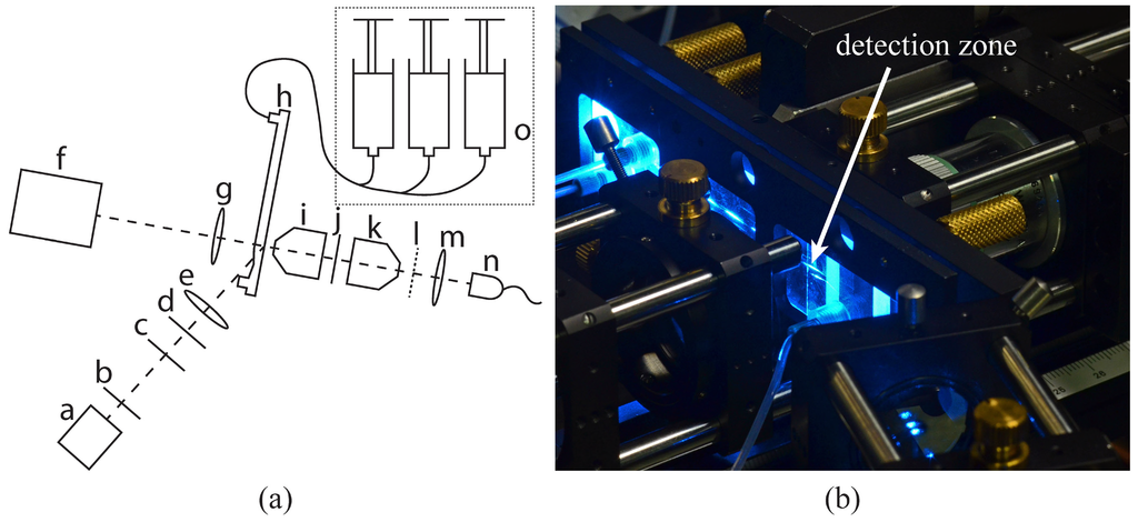
Figure 1.
Experimental apparatus [9]: (a) Sketch of the experimental apparatus: (a) 488 nm laser, (b) iris diaphragm, (c) interference filter (laser clean-up), (d) λ/2-plate, (e) cylindrical lens, (f) alignment camera, (g) spherical lens, (h) microfluidic chip, (i) and (k) microscope objective, (j) interference filter (high-pass), (l) spatially modulated mask, (m) spherical lens, (n) avalanche photo diode, (o) syringe pumps. (b) Microfluidic chip (h) installed in the experimental apparatus during measurement. The detection zone is located at the tip of the arrow.
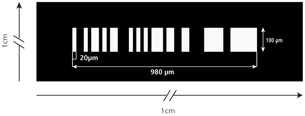
Figure 2.
Sketch [10] of the spatially modulated mask showing the 50-digit binary sequence. The width of each digit is 20 µm. The total mask length is 980 µm starting left of the open feature (#1) and ending right of the last open feature (#49). The last feature (#50) is opaque and therefore not distinguishable from the mask body.
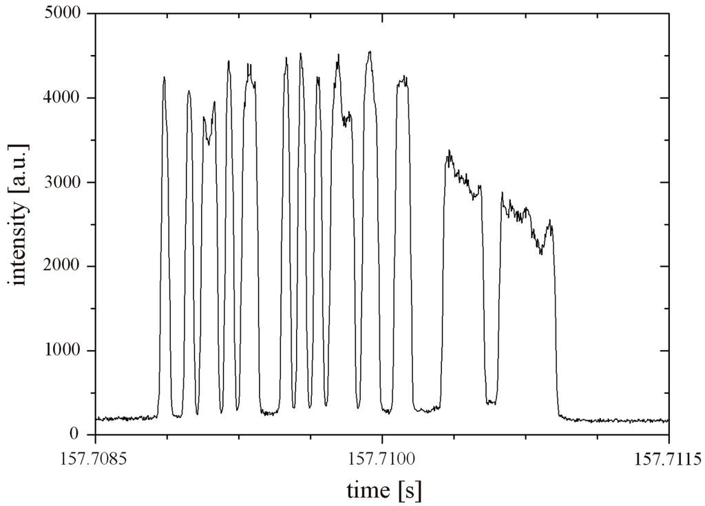
Figure 3.
Signature of a fluorescently stained SUP-B15 cell traversing the mask. It takes ~2 ms for the cell to pass the mask length of 980 µm which corresponds to a velocity of 490 mm/s.
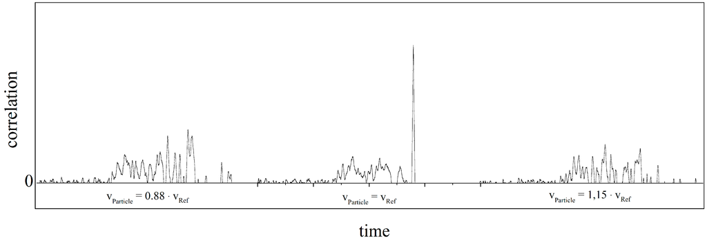
Figure 4.
A sequence of three simulated particles with different velocities when analyzed in a single velocity channel at VRef. The correlation in the center is in resonance (VParticle = VRef) and thus yields the largest main peak amplitude with side lobes located near the main peak. The correlations at the far left (VParticle = 0.88 × VRef) and at the far right (VParticle = 1.15 × VRef) are off-resonance and result in a non-existing main peak and only side lobes.
2.1. The Fluidic Chip
The microfluidic chip is sketched in Figure 5a,b. The measurement channel has a width w = 447 µm, a height d = 12.1 µm and a total length of 7 cm. Port 1 is the inlet for the sample liquid carrying the particles or cells. Ports 2 and 3 are for sheath liquid used to hydrodynamically focus the sample flow to a transport region in the center of the measurement channel (compare Figure 5c). The detection zone is placed 47.5 mm downstream after the junction for hydrodynamic focusing. Port 4 is a liquid outlet connected to a waste container. The high aspect ratio of w/d = 37 has been chosen to create a one-dimensional flow profile over a wide range in y-direction around the center of the measurement channel as demonstrated in Figure 6. For an ideal rectangular channel with w >> d the flow profile is one dimensional in good approximation over a width w–2∙d around the center of the channel. Objects in that region are exposed to a one dimensional flow profile in the sense that the flow profile does not change in y-direction and no shear gradients exist towards the distant side walls of the channel.
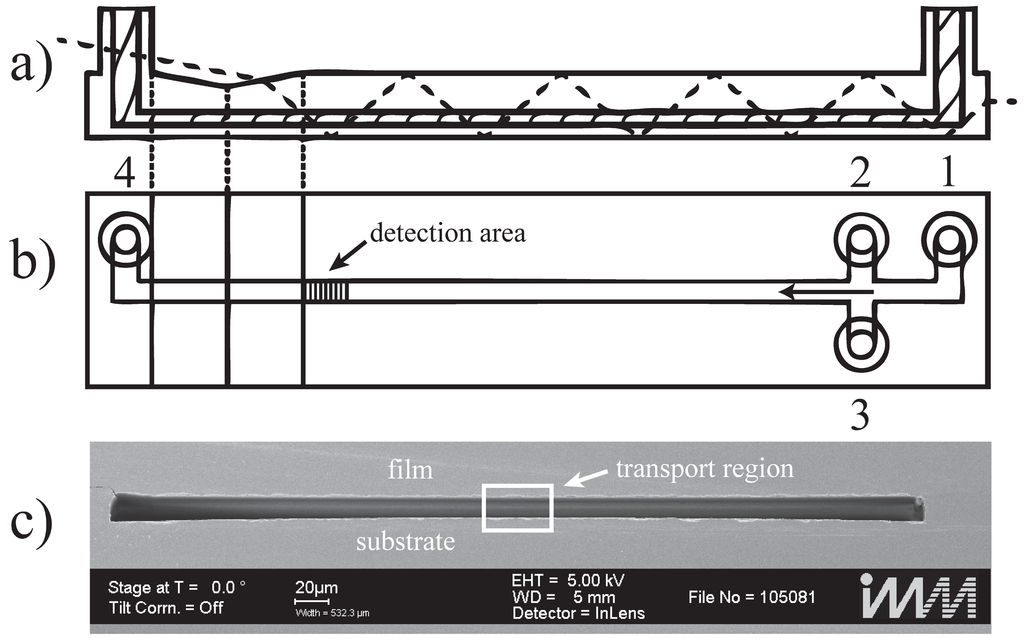
Figure 5.
Microfluidic chip (a) Longitudinal cross section of the microfluidic chip. The shaded area is the microfluidic channel. The optical path of the excitation light is indicated using the dashed line entering in the upper left corner; (b) Channel top view. Port 1 is the connection for the sample syringe; ports 2 and 3 are the inlets for the sheath flow. The arrow in the channel shows the direction of flow. The shaded area indicates the detection area. Port 4 is the outlet; (c) Scanning electron microscope image of the channel cross section of the measurement channel. The highlighted rectangular frame indicates the transport region that contains the actual particles or cells. The wide regions to the left and right carry sheath liquid [11,12].
The microfluidic chip is made of polymethylmethacrylate extruded (PMMA XT) substrate, and the microfluidic channels are imprinted by hot embossing. Physical stress on the plastic chip is exerted on the material during this manufacturing process resulting in residual strain in the final plastic chip. This strain bends the channel bottom and leads to a deformation of the intended rectangular channel cross section (Figure 5c). Consequently, the ideal flow conditions as depicted in Figure 6 are distorted. To assess the effect of the deformation, the flow profile in the channel is simulated approximating the channel bottom with a triangular shape with a channel height of 14.8 µm at both side walls and a height of 12.1 µm in the center, respectively. In Figure 7 the resulting velocity of the fluid is plotted along a horizontal cut through the channel cross section, located exactly at half the channel height at y = 0 (6.05 µm). This plot reveals the maximum velocity vmax of the flow profile in the transport region in the middle of the microfluidic channel (y = 0, see Figure 7). The simulation was performed with a flow rate of 100 µL/min and demonstrates that the velocity near the channel side walls is substantially higher than at the center of the channel due to imperfection of the manufacturing process. In the real channel (Figure 5c), the height varies far less than 0.1 µm over 60 µm in the center.
Therefore, the experimental conditions were chosen such that the transport region was restricted to 20 µm in width to provide the best possible one dimensional parabolic flow profile and to expose all cells/particles to exactly the same hydrodynamic conditions [6]. Additional scanning electron microscope image at various locations along the channel did reveal fluctuations in the channel height below ±0.1 µm and in channel width below ±5 µm. Thus, variations of the flow profile along the channel can be neglected.
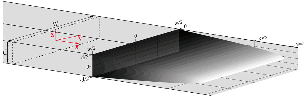
Figure 6.
Parabolic flow profile in a rectangular channel having height d and width w, the dashed line shows the cross section at an arbitrary position in the channel to depict the orientation of the coordinate system (red arrows).
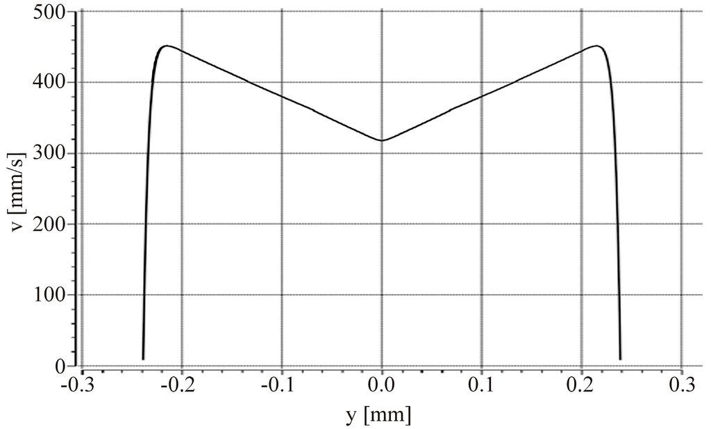
Figure 7.
Simulation of the channel bottom deflection, approximated with a triangle. The simulation shows that, in contrast to the flow profile of a perfect rectangular cross section, the velocity is dependent on y over the total channel width w. The velocity profile corresponds to a horizontal cut through the middle of the channel at position y = 0.
2.2. Equilibrium Velocity
Particles transported in a parabolic flow profile will be exposed to two main forces: the viscous force and the inertial lift force. While the inertial lift force drives the particles towards lower velocities at the channel walls, the drag force pushes them towards higher velocities at the channel center. Thus, particles homogeneously distributed at the channel inlet will exhibit a lateral migration in the z-direction towards a distinct equilibrium position, a phenomenon known as the Segré-Silberberg effect [13,14,15,16] (see Figure 8). The equilibrium position is size dependent as reported by Hur et al. [17] and it can be associated with a corresponding equilibrium velocity in the direction of flow [6].
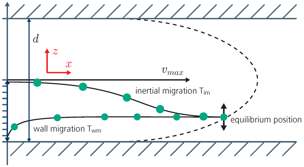
Figure 8.
Longitudinal section of the microfluidic channel with a parabolic flow profile (dashed line). Two competing forces act on a suspended particle. The viscous lift force leads to inertial migration (Tim) while the drag force leads to wall migration Twm in z-direction.
To establish transport of particles at the equilibrium position/velocity, channel Reynolds number, particle size and travel distance in the channel have to be selected appropriately. On the basis of data from the literature [17,18,19,20] we used channel Reynolds numbers of Re = 14.9, Re = 8 and Re = 7.4, respectively. Channel Reynolds number was calculated according to Re = ρ<v>Dh/µ (ρ: density, <v>: average velocity, µ: viscosity, hydraulic diameter: Dh = 2wd/(w + d). Travel distance was set to 47.5 mm (see previous section). Under these experimental conditions particles with diameter above 3 µm reach their equilibrium velocity at the detection area, whereas smaller particles maintain significantly broader distributions [6].
2.3. Particle Suspension
Reference experiments for the effect of particle size on the equilibrium velocity for rigid particles were conducted with a suspension of Fluoresbrite® Polychromatic (PC) Red microsphere particles (diameter 5.51 µm, Polysciences Inc., Warrington, PA, USA) and SPHERO™ Fluorescent Nile Red particles (diameter 0.84 µm and 4.24 µm, Spherotech Inc., Lake Forest, IL, USA). Measurements were performed at 200 µL/min and 100 µL/min at a Reynolds number of 14.9 and 7.4, respectively. The 0.84 µm particles are used to probe the velocity of the flow profile during the measurement, as these particles are too small to be subject to the Segré-Silberberg effect at Reynolds number 7.4 and 14.9. They are therefore broadly distributed over the channel height.
2.4. Bacteria Preparation
Marinococcus luteus was obtained from the German Collection of Microorganism and Cell Cultures (DSMZ). The bacteria were cultured on marine broth agar plate at 28 °C for 72 h. The plates where made out of 41 g marine broth (Carl-Roth), 15 g Agar (Carl-Roth) and solved in 1 L of ultra-pure water. To stain the bacteria with a fluorescent dye, they were harvested and centrifuged at 5000 rpm for 5 min, the pellet was re-suspended in 1 mL phosphate-buffered saline (PBS, Applichem, Germany) and 4 µL of 5 mM carboxyfluorescein succinimidyl ester (CFSE, Invitrogen) and incubated in a water bath at 37 °C for 30 min. Afterwards the bacteria were re-pelleted by centrifugation and re-suspended in 1 mL of fresh PBS. This step was repeated three times. The bacteria suspension was then transferred to the syringe pump of the experimental apparatus. The bacteria measurement was performed at 100 µL/min resulting in a Reynolds number of 7.4.
2.5. Cell Preparation
B-cell precursor leukemia cell line SUP-B15 was obtained from the DSMZ and cultured in McCoy’s 5A Medium (Biochrome, Berlin, Germany) containing 20% heat inactivated fetal calf serum (FCS, Sigma-Aldrich, St. Louis, MO, USA) and 1% GIBCO GlutaMAX™ (dilution 1:100, Life Technologies, Carlsbad, CA, USA). The cells were incubated in humidified atmosphere at 37 °C containing 5% of CO2 and harvested at a concentration of about 1.5 × 10⁶ cells/mL by centrifugation at 450 g for 5 min at room temperature. To stain the cells with a fluorescent dye, the pellet was re-suspended in 1 mL PBS with additional 2 µL of 5 mM CFSE and incubated in a water bath at 37 °C for 15 min. Afterwards, the cells were re-pelleted by centrifugation and re-suspended in 1 mL of fresh PBS and incubated for additional 30 min. Then the PBS was exchanged via centrifugation under the same conditions. Subsequently, the cell suspension was transferred to the syringe pump of the experimental apparatus.
To compare the quality of our results with a commercially available cell counter, we choose the CASY TT cytometer (Roche, Basel, Switzerland). The CASY counter measures size and condition of a cell using the electrical current exclusion (ECE) principle. The intact cell membrane of a viable cell does not conduct electrical current so that the true cell volume is determined. The broken cell membrane of a dead cell is permeable for electrical currents and therefore only the size of the nucleus is measured [21]. For comparable measurements the same passage of cell suspension was analyzed by the CASY counter as well as using the SME technique. The measurement was performed at a total flow rate of 200 µL/min and a Reynolds number of 14.9.
3. Results and Discussion
Figure 9a shows a scatter plot of the intensity of rigid spherical particles as a function of velocity. The data contains results for particles of mean diameters 5.51 µm, 4.42 µm and 0.84 µm. The 0.84 µm as well as the 5.51 µm particles are used to probe the flow profile. The interaction of the 0.84 µm particles with the fluid is low due to their small size. Even at high Reynolds numbers of Rek = 14.9 the particles do not align to a specific equilibrium velocity but are spread over almost the entire height of the channel. The population of 0.84 µm particles provides information about the maximum velocity vmax (see Figure 9b) while viscosity variations across different measurements are monitored via the equilibrium velocity of the 5.51 µm population (for details see [6]). Comparing the 5.51 µm and 4.24 µm population, one can see that both populations clearly differ in velocity with a velocity difference of Δv = 15 mm/s (v(5.51 µm) = 471 ± 2 mm/s, v(4.42 µm) = 486 ± 2 mm/s at vmax = 660 mm/s) at vmax = 660 mm/s). The dim subpopulations above the 0.84 µm and the 4.42 µm population are duplets or triplets of particles.
Cell size similarly affects transport velocity as evidenced by means of the scatter plot in Figure 10 and the corresponding velocity distributions in Figure 11b for the example of SUP-B15 cells. Three dominating populations can be distinguished by intensity as well as by velocity and they are denoted in the plot as “viable cells”, “dead cells” and “debris”. The size distribution of the SUP-B15 cell suspension measured with the CASY counter is shown for comparison in Figure 11a. According to the specifications the CASY counter assigns viable cells in the range between the solid lines, dead cells in the range between the left dashed line (3.5 µm) and the solid line (9 µm) in the middle of Figure 11a. Cell debris is found left of the dashed line for a size of 3.5 µm and below. Thus, the CASY counter measurement results in a total cell count of 1.35 × 10⁶, a viable cells count of 1.15 × 10⁶ leading to a cell viability of 85%.
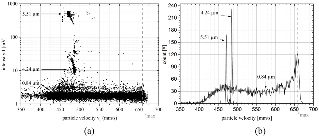
Figure 9.
Particle suspension measurement: (a) Scatter plot of the intensity as a function of particle velocity of a suspension containing particles with mean diameters of 5.51 µm, 4.24 µm and 0.84 µm. The vertical dashed line is an auxiliary line showing the maximum theoretical channel velocity of the center stream line. (b) Velocity distribution of the 0.84 µm, 4.24 µm particles and 5.51 µm particles.
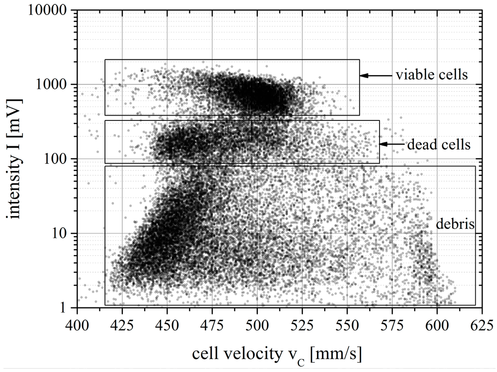
Figure 10.
Intensity versus cell velocity scatter plot of a SUP-B15 cell suspension stained with carboxyfluorescein succinimidyl ester (CFSE) and measured with the spatially modulated emission (SME) method. Each dot corresponds to a measured cell passing the detection zone. The scatter plot shows three clearly separated populations.
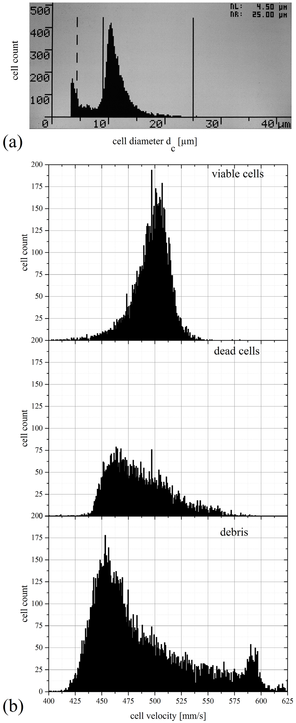
Figure 11.
(a) SUP-B15 size distribution of a CASY counter measurement. The viable cells have their maximum in size at 11 µm, dead cells are measured between the dashed and consistent lines at sizes between 4.5 µm and 9 µm. Debris was measured downwards below 4.5 µm. (b) Velocity distribution of debris, viable and dead SUP-B15 cells measured with the experimental setup. Viable cells reach their mean velocity at 501.4 mm/s, dead cells at 463.6 mm/s. Gating is done via the rectangles in Figure 10.
Viable cells are the largest cells in this suspension with diameters ranging from approximately 8–12 µm. The membrane of these cells is intact and the whole cell membrane and the cytoplasm are stained with the fluorescent dye CFSE. Therefore, these cells are assumed to be brightest and we attribute the brightest population with a mean intensity of 695.4 mV in the SME scatterplot to the viable cells. The viable cells pass the microfluidic channel with a mean velocity of 501.4 mm/s (see Table 1).
The second population identified in the SME plot is attributed to dead or apoptotic cells. In the CASY counter the signal from dead cells is dominated by the size of the cell nucleus due to the measurement principle of electrical current exclusion. The cell membrane of dead cells is broken and cells shrink following the drain of cytoplasm. In the SME results this has two effects: (1) dead cells exhibit lower fluorescence intensity due to the loss of stained cytoplasm and fragments of the cell membrane. Consequently, the dim population distributed around a fluorescent intensity of 181.3 mV is attributed to the dead cells; (2) the shrinking of the cells affects their hydrodynamic transport conditions, resulting in the shift (−37.8 mm/s) of the average velocity of the dead cell population (463.6 mm/s) with respect to the viable cells.

Table 1.
Velocity and intensity for the SUP-B15 cell measurement of Figure 10.
| Population | SUP-B15 Cell Line | |
|---|---|---|
| Velocity (mm/s) | Intensity (mV) | |
| Viable cells | 501.4 | 695.4 |
| Dead cells | 463.6 | 181.3 |
The third population measured by the experimental apparatus is attributed to cell debris. Cell debris is composed of fragments of the membrane and has a wide range of sizes and thus shows a broad distribution in velocity as well as fluorescent intensity. This is the reason for the diagonal skew of the detected population in the scatter plot.
Comparing the measured cell viability of the CASY counter with the cell viability of the experimental apparatus, we recognize that the CASY counter measures a viability of 85% while the SME System records 55%. This indicates that a significant fraction of the cells is damaged by physical stress before they reach the detection zone. An ongoing task is to identify the location in the microfluidic structure causing the cell damage. Furthermore, the viable cell and dead cell distributions overlap, in contrast to the spherical rigid particles (compare Figure 9) where the differently sized particle populations appear at clearly different velocities. This indicates that cell sizes of both populations overlap. The faster cells in the dead cell population may be apoptotic cells which have initiated their programmed cell death. The slower cells in the viable cell population may be young SUP-B15 cells which have not grown to their mature size yet. At further increased channel Reynolds number, the distance between the velocity distributions for rigid particles increases [6]. Thus we expect even clearer results for cell viability assessment at higher channel Reynolds number as long as there is no overlap in physical cell size between viable and dead cells.
Figure 12 compares the velocity distribution for Marinococcus luteus and rigid 0.84 µm particles measured at almost identical Reynolds number of Re = 7.4 and Re = 8, respectively. Marinococcus luteus (spherical shape, size between 0.1 µm and 0.5 µm [8]) exhibits a clear peak at relative velocity v/vmax = 0.77 and a minor peak at maximum velocity (v/vmax = 1), indicating that most of the bacteria have migrated close to the Segré-Silberberg equilibrium position after having travelled 47.5 mm in the microchannel. Some bacteria, however, remain in the center of the channel where the inertial forces are almost cancelled out and these bacteria still travel at the maximum velocity of the flow profile. In contrast to this, the larger 0.84 µm particles are spread over the whole flow profile and no distinct Segré-Silberberg position can be observed. This observation is remarkable, as larger, spherical particles reach the Segré-Silberberg position after shorter traveling distance [7]. We suspect that the deformability of Marinococcus luteus bacteria allows for more effective inertial migration in contrast to the rigid spherical particles. As the bacteria were fixated, active movement can be excluded as well as gravitation due to the microfluidic channel orientation. Detailed investigation on that subject is required to analyze the difference between in dynamics of the inertial migration for deformable and rigid particles.
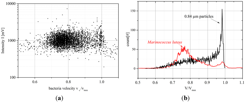
Figure 12.
(a) Intensity versus velocity plot for a suspension of Marinococcus luteus, each dot depicts a single bacterium passing the detection zone (for vc/vmax > 1.05: false positives due to data processing artifacts); (b) Normalized velocity distribution for Marinococcus luteus compared with the velocity distribution of 0.84 µm particles measured under almost identical hydrodynamic conditions (Marinococcus luteus: Re = 8, 0.84 µm particles Re = 7.4).
4. Conclusions
Our results show that cell velocity contains valuable information about physical cell properties such as size. This information can be used to distinguish between different cell conditions. The results of the SME technique are in that sense comparable with those of the commercially available CASY TT counter. Consequently, velocimetry offers access to additional parameters for microfluidic flow cytometers without adding significant cost or complexity to the system, especially when using the SME technique.
An ongoing task is the optimization of the microfluidic channel to eliminate the deformation of the channel cross-section and thus to eliminate the need for a sheath flow. Utilizing the full channel width for cell transport is prerequisite to harvest the full potential of the SME technique for processing high sample volume and gaining meaningful information from the cell velocity. The bacteria measurements indicate that deformable objects migrate to their equilibrium position faster than rigid spherical particles. Detailed investigations on the dynamics of the lateral migration of rigid and deformable particles are required.
Acknowledgments
The authors thank Tobias Broger for realizing an extremely reliable and fail-safe data sampling system and Stephan Schmitt whose knowledge in silicon-based thin film technology was the key to fabricating precise microfluidic channels. Furthermore we thank Karl-Peter Schelhaas for the simulation of the channel bottom deflection. We also thank Markus Wink and Mareike Bürger for proofreading the text. The European Research Council (ERC) is acknowledged for funding the project under grant #258604.
Author Contributions
Christian Sommer and Michael Baßler conceived and designed the experiments; Christian Sommer, Lisa Schott and Khaliun Myagmar performed the experiments; Christian Sommer, Lisa Schott, Thomas Walther and Michael Baßler analyzed the data; Lisa Schott, Christian Sommer contributed reagents/materials/analysis tools; Lisa Schott, Joern Wittek, Thomas Walther and Michael Baßler wrote the paper.
Conflicts of Interest
The authors declare no conflict of interest.
References and Notes
- Shapiro, H.M. Practical Flow Cytometry, 4th ed.; John Wiley and Sons: Hoboken, NJ, USA, 2003. [Google Scholar]
- Piyasena, M.E.; Graves, S.W. The intersection of flow cytometry with microfluidics and microfabrication. Lab Chip 2014, 14, 1044–1059. [Google Scholar] [CrossRef] [PubMed]
- Chung, T.D.; Kim, H.C. Recent advances in miniaturized microfluidic flow cytometry for clinical use. Electrophoresis 2007, 28, 4511–4520. [Google Scholar] [CrossRef] [PubMed]
- Bassler, M.; Kiesel, P.; Schmidt, O.; Johnson, N.M. Method and system implementing spatially modulated excitation or emission for particle characterization with enhanced sensitivity. U.S. Patent 2008/0181827 A1, 31 July 2008. [Google Scholar]
- Kiesel, P.; Bassler, M.; Beck, M.; Johnson, N. Spatially modulated fluorescence emission from moving particles. Appl. Phys. Lett. 2009, 94, 041107. [Google Scholar] [CrossRef]
- Sommer, C.; Quint, S.; Spang, P.; Walther, T.; Baßler, M. The equilibrium velocity of spherical particles in rectangular microfluidic channels for size measurement. Lab Chip 2014, 14, 2319–2326. [Google Scholar] [CrossRef] [PubMed]
- Sommer, C.; Quint, S.; Spang, P.; Walther, T.; Baßler, M. Studying the Segré- Silberberg effect by velocimetry in microfluidic channels. In Advances in Fluid Mechanics X; Brebbia, C.A., Hernández, S., Rahman, M., Eds.; WIT Press: Southampton, UK, 2014; pp. 265–277. [Google Scholar]
- Wang, Y.; Cao, L.; Tang, S.; Lou, K.; Mao, P.; Jin, X.; Jiang, C.; Xu, L.; Li, W. Int. J. Syst. Evol. Microbiol. 2009, 59, 2875–2879. [CrossRef]
- “Sketch of the experimental setup” by Christian Sommer is licensed under CC BY 3.0, published by The Royal Society of Chemistry, Lab Chip 2014, 14, 2319–2326.
- “Sketch of the optical mask generated from the LABS 50” by Christian Sommer is licensed under CC BY 3.0, published by The Royal Society of Chemistry, Lab Chip 2014, 14, 2319–2326.
- “Sketch of the fluidic chip” by Christian Sommer is licensed under CC BY 3.0, published by The Royal Society of Chemistry, Lab Chip 2014, 14, 2319–2326.
- “REM picture of the channel cross section in the fluidic chip” by Christian Sommer is licensed under CC BY 3.0, published by The Royal Society of Chemistry, Lab Chip 2014, 14, 2319–2326.
- Segré, G.; Silberberg, A. Radial Particle Displacements in Poiseuille Flow of Suspensions. Nature 1961, 189, 209–210. [Google Scholar] [CrossRef]
- Segré, G.; Silberberg, A. Behaviour of macroscopic rigid spheres in Poiseuille flow Part 2. Experimental results and interpretation. J. Fluid Mech. 1962, 14, 136–157. [Google Scholar] [CrossRef]
- Goldsmith, H.; Mason, S.G. The flow of suspensions through tubes. I. Single spheres, rods, and discs. J. Colloid Sci. 1962, 17, 448–476. [Google Scholar] [CrossRef]
- Karnis, A.; Goldsmith, H.; Mason, S.G. The kinetics of flowing dispersions. J. Colloid Interface Sci. 1966, 22, 531–553. [Google Scholar] [CrossRef]
- Hur, S.C.; Henderson-MacLennan, N.K.; McCabe, E.R.B.; Di Carlo, D. Deformability-based cell classification and enrichment using inertial microfluidics. Lab Chip 2011, 11, 912–920. [Google Scholar] [CrossRef] [PubMed]
- Gossett, D.R.; Tse, H.T.K.; Dudani, J.S.; Goda, K.; Woods, T.A.; Graves, S.W.; Di Carlo, D. Inertial manipulation and transfer of microparticles across laminar fluid streams. Small 2012, 8, 2757–2764. [Google Scholar] [CrossRef] [PubMed]
- Halow, J.S.; Wills, G.B. Radialmigration of spherical particles in couette systems. AIChE J. 1970, 16, 281–286. [Google Scholar] [CrossRef]
- Hur, S.C.; Tse, H.T.K.; Di Carlo, D. Sheathless inertial cell ordering for extremethroughput low cytometry. Lab Chip 2010, 10, 274–280. [Google Scholar] [CrossRef] [PubMed]
- Roche Diagnostics Corporation. CASY Model TTC—Cell Counter and Analyzer. Available online: http://lifescience.roche.com/wcsstore/RASCatalogAssetStore/Articles/05966680001_04.10_US.pdf (accessed on 21 May 2015).
© 2015 by the authors; licensee MDPI, Basel, Switzerland. This article is an open access article distributed under the terms and conditions of the Creative Commons Attribution license (http://creativecommons.org/licenses/by/4.0/).