A Bayesian Data Fusion Approach to Spatio-Temporal Fusion of Remotely Sensed Images

Abstract

Remote sensing provides rich sources of data for the monitoring of land surface dynamics. However, single-sensor systems are constrained from providing spatially high-resolution images with high revisit frequency due to the inherent sensor design limitation. To obtain images high in both spatial and temporal resolutions, a number of image fusion algorithms, such as spatial and temporal adaptive reflectance fusion model (STARFM) and enhanced STARFM (ESTARFM), have been recently developed. To capitalize on information available in a fusion process, we propose a Bayesian data fusion approach that incorporates the temporal correlation information in the image time series and casts the fusion problem as an estimation problem in which the fused image is obtained by the Maximum A Posterior (MAP) estimator. The proposed approach provides a formal framework for the fusion of remotely sensed images with a rigorous statistical basis; it imposes no requirements on the number of input image pairs; and it is suitable for heterogeneous landscapes. The approach is empirically tested with both simulated and real-life acquired Landsat and Moderate Resolution Imaging Spectroradiometer (MODIS) images. Experimental results demonstrate that the proposed method outperforms STARFM and ESTARFM, especially for heterogeneous landscapes. It produces surface reflectances highly correlated with those of the reference Landsat images. It gives spatio-temporal fusion of remotely sensed images a solid theoretical and empirical foundation that may be extended to solve more complicated image fusion problems.

1. Introduction

Remote sensing provides crucial data sources for the monitoring of land surface dynamics such as vegetation phenology and land-cover changes. Effective terrestrial monitoring requires remotely sensed images high in both spatial and temporal resolutions. However, technological limitations pose challenges [1] for sensor designs, and trade-offs have to be made to balance spatial details with the spatial extent and revisit frequency. For instance, high spatial resolution (henceforth referred to as “high-resolution”) images obtained by the Thematic Mapper (TM) sensor or Enhanced Thematic Mapper Plus (ETM+) sensor on Landsat have a spatial resolution of approximately 30 m and have been shown to be useful in applications such as monitoring of land-cover changes. However, Landsat satellites have a revisit cycle of 16 days, and around 35% of the images are contaminated by cloud cover [2]. Together with other poor atmospheric conditions, this limits the applications of Landsat data. On the contrary, a low spatial resolution (henceforth referred to as “low-resolution”) sensor, such as the Moderate Resolution Image Spectroradiometer (MODIS) on the Aqua and Terra satellites, has a daily revisit period but a relatively low spatial resolution ranging from 250 m to 1000 m, limiting its effectiveness in the monitoring of ecosystem dynamics in heterogeneous landscapes.

To capitalize on the strengths of individual sensors, it is of great advantage to fuse multi-sensor data to generate images high in both spatial and temporal resolutions for the monitoring of dense land surface dynamics, keeping in mind that images acquired by multi-sensors may have different acquisition times, different resolutions (e.g., spectral and radiometric), and different bands (e.g., the number of bands, the central wavelengths, and the bandwidths). Driven by the great potential of applications in various areas, the fusion of multi-sensor data has attracted much attention in recent years [3]. A number of approaches for the spatio-temporal fusion of images have been developed [4].

The spatial and temporal adaptive reflectance fusion model (STARFM) is one of the first fusion algorithms that has been widely used for synthesizing Landsat and MODIS imageries [5]. STARFM does not explicitly treat the issue that sensor difference can change for different land-cover types. An improved STARFM was proposed to address this issue by using linear regression models [6]. Roy et al. [7] proposed a semi-physical fusion approach that explicitly handles the directional dependence of reflectance described by the bidirectional reflectance distribution function (BRDF). STARFM is developed on the assumption of homogeneous pixels, and thus may not be suitable for heterogeneous land surfaces [8]. An enhanced STARFM, termed ESTARFM [9], was developed to improve the prediction of surface reflectance in heterogeneous landscapes, followed by a modified version of ESTARFM that combines additional land-cover data [10]. STARFM and ESTARFM are shown to be useful in capturing reflectance changes due to changes in vegetation phenology [11,12,13,14], which is a key element of seasonal patterns of water and carbon exchanges between land surfaces and the atmosphere [15,16,17]. However, STARFM and ESTARFM may have problems in mapping disturbance events when land-cover changes are transient and not recorded in at least one of the baseline high-resolution (e.g., Landsat) images [8]. An improved method based on STARFM, named spatial temporal adaptive algorithm for mapping reflectance changes (STAARCH), was proposed to detect the disturbance and reflectance changes over vegetated land surfaces by tasseled cap transformation [18]. Similarly, another approach was developed for near real-time monitoring of forest disturbances through the fusion of MODIS and Landsat images [19]. However, this algorithm was developed specifically for forest disturbances. It may not be suitable for other kinds of land-cover changes [20,21]. In contrast to STARFM, both STAARCH and ESTARFM require at least two high-resolution images; that is, one before and another after the target image [22]. However, it is difficult to meet this need for areas with frequently cloudy days [23]. Furthermore, the assumption in ESTARFM that land surface reflectance changes linearly over time with a single rate between two acquired Landsat images may not hold in some cases [8].

Besides the abovementioned algorithms, several methods based on sparse representation and dictionary learning have been proposed [24,25,26]. Although these methods can well predict pixels with land-cover changes, they do not accurately maintain the shape of objects [27]. In addition, the use of strong assumptions on the dictionaries and sparse coding coefficients may not hold in some cases [26].

Another popular branch of image fusion algorithms relies on the unmixing techniques due to their ability to reconstruct images with high spectral fidelity [28,29,30,31,32]. An advantage of the unmixing-based methods is that they do not require high- and low-resolution images to have corresponding spectral bands, and they can downscale extra spectral bands in low-resolution images to increase the spectral resolution of the high-resolution images [30]. In recent years, several approaches have been developed by combining the unmixing algorithm and the STARFM method or other techniques for improved fusion performance [27,29,33,34,35].

Despite that the approaches mentioned above are well developed and widely used, studies on the effectiveness and applicability of applying the Bayesian estimation theory to the spatio-temporal image fusion problems are scanty [36,37,38]. In these studies [36,37,38], linear regression is used to reflect the temporal dynamics, which, however, may not hold in a variety of situations. Moreover, there may be no regression-like trends in some cases. In addition, the Bayesian method can handle uncertainties of input images in a probabilistic manner, which has shown its effectiveness in spatial–spectral fusion of remotely sensed images [39,40,41,42,43,44] and superresolution of remote-sensing images [45,46,47]. It is reasonable to explore the potential of Bayesian approach in spatio-temporal fusion due to its satisfactory performance in the spatial–spectral fusion of remotely sensed images. Although a few Bayesian algorithms have been developed [36,37,38], there lacks a solid theoretical Bayesian framework with rigorous statistical procedures for the spatio-temporal fusion of remotely sensed images. This paper is aimed to develop a Bayesian data fusion framework which provides a formal construct to systematically obtain the targeted high-resolution image on the basis of a solid probabilistic foundation that enables us to efficiently handle uncertainties by applying the statistical estimation tools developed in our model. Our Bayesian fusion approach to the spatio-temporal fusion of remotely sensed images makes use of the advantage of multivariate arguments in statistics to handle temporal dynamics in a more flexible way rather than just by linear regression. Specifically, we use the joint distribution to embody the covariate information that implicitly expresses the temporal changes of images. This approach imposes no requirements on the number of high-resolution images in the input and can generate high-resolution-like images in homogeneous or relatively heterogeneous areas. Our proposed Bayesian approach will be empirically compared with STARFM and ESTARFM [5,9] through quantitative assessment.

The remainder of the paper is organized as follows. We first provide the theoretical formulation of our Bayesian estimation approach in Section 2. Specific considerations for parameter estimations are described in Section 3. In Section 4, we demonstrate the effectiveness of our proposed approach with experimental studies, including the characteristics of the datasets, the quantitative assessment metrics, and the comparison with STARFM and ESTARFM. Section 5 provides further discussion on the results in Section 4 and limitations of this work. We then conclude our paper with a summary in Section 6.

2. Theoretical Basis of Bayesian Data Fusion

Suppose the high- and low-resolution images acquired at the same dates are comparable with each other after radiometric calibration and geometric rectification, and they share similar spectral bands. Denote the set of all available high-resolution images by $\mathscr{H}$ = {H^(s): s $\in$ T_H} and the existing low-resolution images by $ℒ$ = {L^(t), t $\in$ T_L}, where the superscripts s and t represent the acquisition dates of the high- and low-resolution images, respectively. In particular, it is reasonable to assume that the domain of $\mathscr{H}$ is a subset of that of $ℒ$, namely, T_H $\subseteq$ T_L since the high-resolution images generally have lower revisit frequency than the low-resolution images. The objective of this paper is to obtain the image sequence $ℱ$ = {F^(r), r $\in$ T_F}, which has the same spatial resolution with $\mathscr{H}$ and the temporal frequency with $ℒ$, i.e., T_F = T_L, by fusing the corresponding images in $\mathscr{H}$ and $ℒ$.

We assume that each high-resolution image (i.e., H^(s), s $\in$ T_H) has N pixels per band, and each low-resolution image (i.e., L^(t), t $\in$ T_L) has M pixels per band. They have K corresponding spectral bands in this study. The three-dimensional (data cube) images H^(s), L^(t), and F^(r) are represented by the one-dimensional statistical random vectors x^(s), y^(t), and z^(r), composed of the pixels of the images H^(s), L^(t), and F^(r) in the band-interleaved-by-pixel lexicographical order. Their respective expressions are:

$$x^{(s)}={[x_{1,1}^{(s)},...,x_{K,1}^{(s)},x_{1,2}^{(s)},...,x_{K,2}^{(s)},...,x_{1,N}^{(s)},...,x_{K,N}^{(s)}]}^{\mathrm{T}}={[{(x_1^{(s)})}^{\mathrm{T}},{(x_2^{(s)})}^{\mathrm{T}},...,{(x_N^{(s)})}^{\mathrm{T}}]}^{\mathrm{T}}$$

(1)

$$y^{(t)}={[y_{1,1}^{(t)},...,y_{K,1}^{(t)},y_{1,2}^{(t)},...,y_{K,2}^{(t)},...,y_{1,M}^{(t)},...,y_{K,M}^{(t)}]}^{\mathrm{T}}={[{(y_1^{(t)})}^{\mathrm{T}},{(y_2^{(t)})}^{\mathrm{T}},...,{(y_M^{(t)})}^{\mathrm{T}}]}^{\mathrm{T}},$$

(2)

$$z^{(r)}={[z_{1,1}^{(r)},...,z_{K,1}^{(r)},z_{1,2}^{(r)},...,z_{K,2}^{(r)},...,z_{1,N}^{(r)},...,y_{K,N}^{(r)}]}^{\mathrm{T}}={[{(z_1^{(r)})}^{\mathrm{T}},{(z_2^{(r)})}^{\mathrm{T}},...,{(z_N^{(r)})}^{\mathrm{T}}]}^{\mathrm{T}},$$

(3)

where $x_i^{(s)}={[x_{1,i}^{(s)},...,x_{k,i}^{(s)},...,x_{K,i}^{(s)}]}^{\mathrm{T}}$ is the vector of pixels for all K bands at pixel location i of the high-resolution image on date s, i = 1, …, N, within which $x_{k,i}^{(s)}$ is the pixel value of band k at location i on date s; $y_j^{(t)}={[y_{1,j}^{(t)},...,y_{k,j}^{(t)},...,y_{K,j}^{(t)}]}^{\mathrm{T}}$, j = 1, …, M, and $z_i^{(r)}={[z_{1,i}^{(r)},...,z_{k,i}^{(r)},...,z_{K,i}^{(r)}]}^{\mathrm{T}}$, i = 1, …, N, are defined similarly.

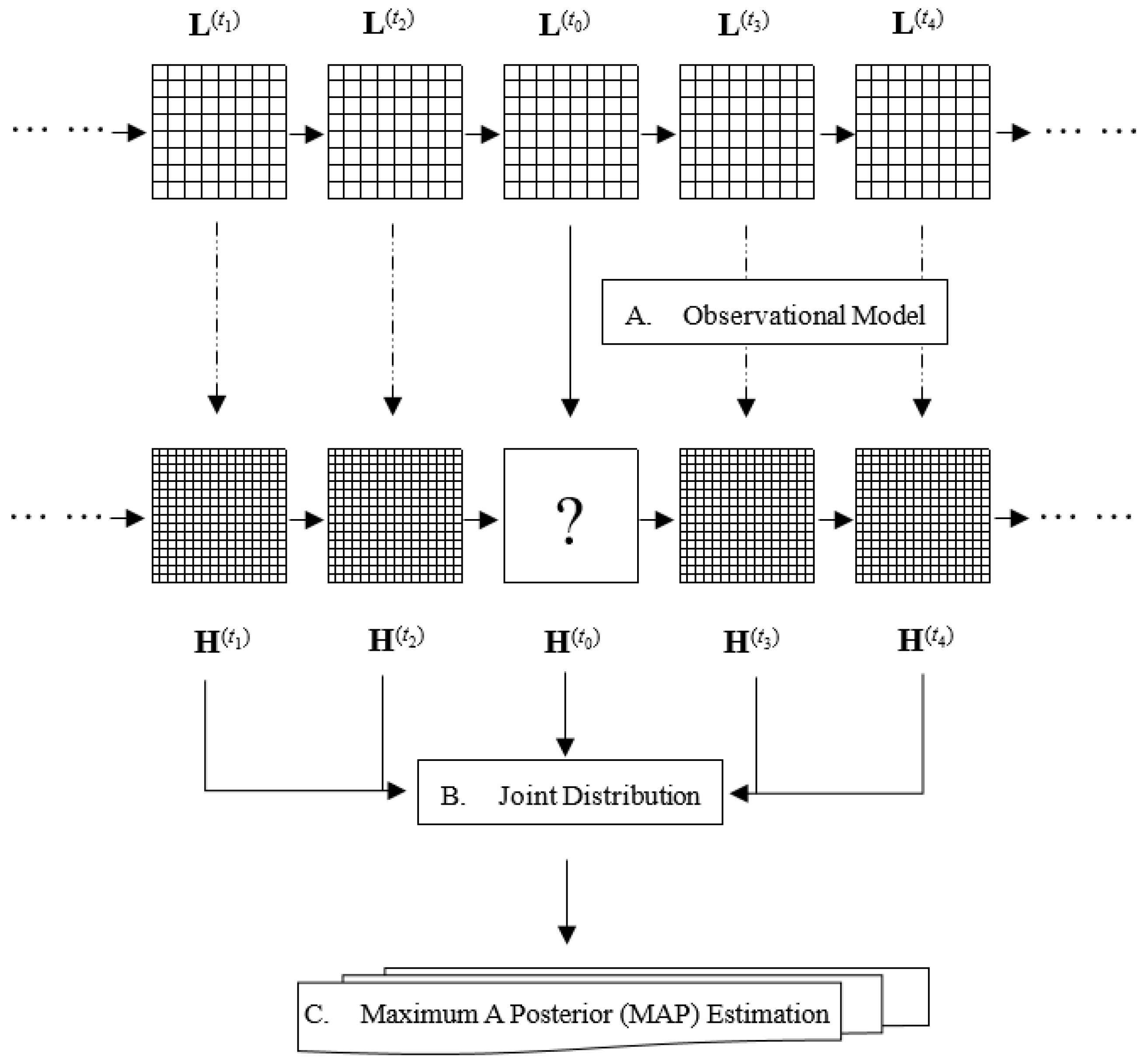
To be specific, we assume the target high-resolution image is missing on date t₀ and available on dates t_k, k = 1, …, S, that is, t₀ $\notin$ T_H and t_k $\in$ T_H, while the low-resolution images are available on both t₀ and t_k. Our objective is to estimate $z^{(t_0)}$ given the corresponding $y^{(t_0)}$ at the target date t₀ and the other image pairs $x^{(t_k)}$ and $y^{(t_k)}$. In this section, we propose a general framework for Bayesian data fusion depicted in Figure 1. Part A of Figure 1 models the relationship between the low-resolution and high-resolution images at the target date t₀. Part B shows the use of multivariate joint distribution to model the evolution of the images and their temporal correlations. Finally, the targeted high-resolution image is estimated by the Maximum A Posterior (MAP) estimation as shown in part C.

Figure 1. The general framework of Bayesian data fusion using quadruple pairs. It should be noted that the framework can be extended to the use of any number of image-pairs, even just one pair.

In what follows, we give a detail description of the components of the general framework.

2.1. The Observation Model

The basic concept of Bayesian data fusion comes from the idea that variables of interest cannot be directly observed. Thus, it is necessary to model the relationship between variables available and variables of interest, which are unknown. The first step of our approach is to build a model to describe the relationship between the low-resolution image and the high-resolution image at the target date t₀. We call it the observational model, which can be written in a matrix form as [48,49]:

$$y^{(t_0)}=DB{z}^{(t_0)}+e^{(t_0)}=W{z}^{(t_0)}+e^{(t_0)},$$

(4)

where W = DB is the KM $\times$ KN transformation matrix, D is the KM × KN down-sampling matrix, B is the KN × KN blurring matrix, and $e^{(t_0)}$ is the noise. The effects of blurring and down-sampling of the target high-resolution image are combined into the point spread function (PSF) W, which maps the pixels of the high-resolution image to the pixels of the low-resolution image [38,50]. Each low-resolution pixel is assumed to be the convolution of the high-resolution pixels with the PSFs expressed as the rows in W plus noise $e^{(t_0)}$.

In this study, W is assumed to be a rectangular PSF model, similar to the approach in [51]. This approach proves to be effective. The PSF for each low-resolution pixel is uniform and also non-overlapping among neighboring low-resolution pixels. Specifically, it is defined with an equal weight of $1/w^2$ for the high-resolution pixels contained within the same low-resolution pixel, where w = n/m is the resolution ratio, and n $\times$ n = N, m $\times$ m = M. Note that N and M are perfect squares. So the form of W can be expressed by the matrix operation

$$W_{MK\times NK}=1/w^2·H_{m\times n}\otimes G_{mK\times nK},$$

(5)

where,

$$H_{m\times n}=I_{m\times m}\otimes 1_{1\times w},$$

$$G_{mK\times nK}=I_{m\times m}\otimes 1_{1\times w}\otimes I_{K\times K}$$

The items $I_{m\times m}$ and $I_{K\times K}$ are respectively the m-dimensional and K-dimensional unit matrix. The item $1_{1\times w}$ is a w-dimensional row vector with unit values, and $\otimes$ is the Kronecker product of matrices.

The random vector e is assumed to be a zero-mean Gaussian random vector with a covariance matrix $C_{e^{(t_0)}}$. The probability density function for $e^{(t_0)}$ is expressed as:

$$p(e^{(t_0)})=1/\sqrt{{(2\pi )}^{MK}|C_{e^{(t_0)}}|}\exp \{-\frac{1}{2}{e}^{(t_0)\mathrm{T}}{C}_{e^{(t_0)}}^{-1}{e}^{(t_0)}\}.$$

(6)

In most applications, it is reasonable to assume that the noise is independent and identically distributed from band-to-band and pixel-to-pixel, which means that the covariance matrix is diagonal with $C_{e^{(t_0)}}$ = ${\sigma }_e^2$I. It is reasonable to assume that the sensor noise is independent of both $z^{(t_0)}$ and $x^{(t_k)}$, t_k $\in$ T_H $\subseteq$ T_L, k = 1, …, S, because it comes from the acquisition of $y^{(t_0)}$.

This observational model incorporates knowledge about the relationships between the low-resolution and high-resolution images at the target date and the variability caused by the noise. Without other information, this model-based approach for estimating $z^{(t_0)}$ is ill-posed because the dimension of the unknowns is greater than the dimension of the equations. Thus, it is necessary to include additional information about the desirable high-resolution image, which is provided by the existing high-resolution images in $\mathscr{H}$, into the calibration process.

2.2. The Joint Distribution

The temporal correlation of time-series images depends on the dynamics of the land surface. It is relatively low for situations with rapid phenology changes or sudden land-cover changes due to, for example, forest fires or floods. Previous regression approaches [36,37,38] use a linear relationship to represent the temporal evolution of the image sequences, which may not hold for cases with rapid phenology changes or sudden land-cover changes. In this paper, we treat the temporal evolution of images as a stochastic process and employ the notion of multivariate joint Gaussian distribution to model it. This approach can be applied to cases with nonlinear temporal evolution and is thus more general than the regression approach. To take advantage of the temporal correlation of image sequences, we assume $x^{(t_k)}$ (the same with $z^{(t_k)}$), t_k $\in$ T_H $\subseteq$ T_L, k = 1, …, S, and $z^{(t_0)}$, t₀ $\in$ T_L but t₀ $\notin$ T_H, are jointly Gaussian distributed, and define an NKS-dimensional vector X by cross-combining the S high-resolution image vectors:

$$X={[{(x_1^{(t_1)})}^{\mathrm{T}},{(x_1^{(t_2)})}^{\mathrm{T}},...,{(x_1^{(t_S)})}^{\mathrm{T}},{(x_2^{(t_1)})}^{\mathrm{T}},...,{(x_2^{(t_S)})}^{\mathrm{T}},...,{(x_N^{(t_1)})}^{\mathrm{T}},...,{(x_N^{(t_S)})}^{\mathrm{T}}]}^{\mathrm{T}}={[X_1^{\mathrm{T}},X_2^{\mathrm{T}},...,X_N^{\mathrm{T}}]}^{\mathrm{T}}$$

Then based on the conditional property of the multivariate Gaussian distribution, the conditional probability density function is also Gaussian which can be expressed as [52]:

$$p(z^{(t_0)}|x^{(t_1)},...,x^{(t_s)})=p(z^{(t_0)}|X)=1/\sqrt{{(2\pi )}^{NK}|C_{z^{(t_0)}|X}|}\exp \{-\frac{1}{2}{(z^{(t_0)}-{\mathsf{\mu }}_{z^{(t_0)}|X})}^{\mathrm{T}}{C}_{z^{(t_0)}|X}^{-1}(z^{(t_0)}-{\mathsf{\mu }}_{z^{(t_0)}|X})\},$$

(7)

where ${\mathsf{\mu }}_{z^{(t_0)}|X}$ is the conditional expectation of $z^{(t_0)}$ given the existing high-resolution sequences X, and $C_{z^{(t_0)}|X}$ is the conditional covariance matrix of $z^{(t_0)}$ given X. They can be calculated by the joint statistics

$${\mathsf{\mu }}_{z^{(t_0)}|X}=\mathrm{E}\{z^{(t_0)}\}+C_{z^{(t_0)},X}{C}_{X,X}^{-1}(X-\mathrm{E}\{X\}),$$

(8)

$$C_{z^{(t_0)}|X}=C_{z^{(t_0)},z^{(t_0)}}-C_{z^{(t_0)},X}{C}_{X,X}^{-1}{C}_{z^{(t_0)},X}^{\mathrm{T}},$$

(9)

where $\mathrm{E}\{X\}$ is the mean of X and $\mathrm{E}\{z^{(t_0)}\}$ is the mean of $z^{(t_0)}$. The matrices $C_{X,X}$, $C_{z^{(t_0)},X}$, and $C_{z^{(t_0)},z^{(t_0)}}$ are the cross-covariance matrices of the corresponding multivariate random vectors, respectively.

2.3. The MAP Estimation

Here the goal of the MAP estimation of the Bayesian framework is to obtain the desirable high-resolution image $z^{(t_0)}$ at the target date by maximizing its conditional probability relative to the existing high-resolution sequences X and the observed low-resolution image $y^{(t_0)}$ at the target date. It can be given as:

$${\widehat{\mathbf{z}}}^{(t_0)}=\underset{z^{(t_0)}}{\arg \max }p(z^{(t_0)}|y^{(t_0)},X),$$

(10)

where $p(z^{(t_0)}|y^{(t_0)},X)$ is the conditional probability density function of $z^{(t_0)}$ given $y^{(t_0)}$ and X, and the optimal ${\widehat{\mathbf{z}}}^{(t_0)}$ is the MAP estimate of $z^{(t_0)}$ that maximizes $p(z^{(t_0)}|y^{(t_0)},X)$. According to the Bayes rule, we have

$$p(z^{(t_0)}|y^{(t_0)},X)=(p(y^{(t_0)},X|z^{(t_0)})·p(z^{(t_0)}))/p(y^{(t_0)},X)=p(y^{(t_0)}|z^{(t_0)})·p(X|z^{(t_0)})·p(z^{(t_0)})/p(y^{(t_0)},X).$$

Again using the Bayes rule on $p(X|z^{(t_0)})$ we yield $p(X|z^{(t_0)})=(p(z^{(t_0)}|X)·p(X))/p(z^{(t_0)})$. Substituting them into (10), the MAP estimator can be rewritten as:

$${\widehat{\mathbf{z}}}^{(t_0)}=\underset{z^{(t_0)}}{\arg \max }p(y^{(t_0)}|z^{(t_0)})·p(z^{(t_0)}|X).$$

(11)

Based on the observational model in (4) and the probability density function of noise in (6), we obtain

$$p(y^{(t_0)}|z^{(t_0)})=1/\sqrt{{(2\pi )}^{MK}|C_{e^{(t_0)}}|}\exp \{-\frac{1}{2}{(y^{(t_0)}-W{z}^{(t_0)})}^{\mathrm{T}}{C}_{e^{(t_0)}}^{-1}(y^{(t_0)}-W{z}^{(t_0)})\}.$$

(12)

Given that the conditional probability density functions in (7) and (12) are Gaussian distribution, obviously their product, $p(y^{(t_0)}|z^{(t_0)})·p(z^{(t_0)}|X)$, is also a Gaussian distribution with mean

$$\widehat{\mathsf{\mu }}=\widehat{\mathbf{C}}[W^{\mathrm{T}}{C}_{e^{(t_0)}}^{-1}{y}^{(t_0)}+C_{z^{(t_0)}|X}^{-1}{\mathsf{\mu }}_{z^{(t_0)}|X}],$$

and covariance

$$\widehat{\mathbf{C}}={[W^{\mathrm{T}}{C}_{e^{(t_0)}}^{-1}W+C_{z^{(t_0)}|X}^{-1}]}^{-1}.$$

Lastly, the optimal estimator of the desirable high-resolution image ${\widehat{\mathbf{z}}}^{(t_0)}$ is given by

$${\widehat{\mathbf{z}}}^{(t_0)}={[W^{\mathrm{T}}{C}_{e^{(t_0)}}^{-1}W+C_{z^{(t_0)}|X}^{-1}]}^{-1}[W^{\mathrm{T}}{C}_{e^{(t_0)}}^{-1}{y}^{(t_0)}+C_{z^{(t_0)}|X}^{-1}{\mathsf{\mu }}_{z^{(t_0)}|X}].$$

(13)

In order to reduce the memory space and computational cost and to avoid the problem of the inversion of the noise covariance matrix in (6) going to zero, we apply the matrix inversion lemma [52] to simplify (13) to obtain:

$${\widehat{\mathbf{z}}}^{(t_0)}={\mathsf{\mu }}_{z^{(t_0)}|X}+C_{z^{(t_0)}|X}{W}^{\mathrm{T}}{[W{C}_{z^{(t_0)}|X}{W}^{\mathrm{T}}+C_{e^{(t_0)}}]}^{-1}[y^{(t_0)}-W{\mathsf{\mu }}_{z^{(t_0)}|X}].$$

(14)

3. Implementation Considerations

In terms of the temporal correlation of image sequences, we have weakened the assumption of the joint Gaussian distribution for the whole high-resolution image vectors to N joint Gaussian distributions for each high-resolution pixel series. This simplification can greatly reduce the calibration of the algorithm. Therefore, the conditional mean vector ${\mathsf{\mu }}_{z^{(t_0)}|X}$ and covariance matrix $C_{z^{(t_0)}|X}$ can be estimated for each individual pixel [40] as:

$${\mathsf{\mu }}_{z^{(t_0)}|X}={[{\mathsf{\mu }}_{z_1^{(t_0)}|X_1}^{\mathrm{T}},{\mathsf{\mu }}_{z_2^{(t_0)}|X_2}^{\mathrm{T}},...,{\mathsf{\mu }}_{z_N^{(t_0)}|X_N}^{\mathrm{T}}]}^{\mathrm{T}},$$

(15)

$$C_{z^{(t_0)}|X}=\left[\begin{array}{cccc}{C}_{z_1^{(t_0)}|X_1}& 0& \cdots & 0\\ 0& C_{z_2^{(t_0)}|X_2}& & ⋮\\ ⋮& & \ddots & 0\\ 0& \cdots & 0& C_{z_N^{(t_0)}|X_N}\end{array}\right],$$

(16)

where

$${\mathsf{\mu }}_{z_i^{(t_0)}|X_i}=\mathrm{E}\{z_i^{(t_0)}\}+C_{z_i^{(t_0)},X_i}{C}_{X_i,X_i}^{-1}(X_i-\mathrm{E}\{X_i\}),$$

(17)

$$C_{z_i^{(t_0)}|X_i}=C_{z_i^{(t_0)},z_i^{(t_0)}}-C_{z_i^{(t_0)},X_i}{C}_{X_i,X_i}^{-1}{C}_{z_i^{(t_0)},X_i}^{\mathrm{T}},$$

(18)

and the pre-defined $X_i={[{(x_i^{(t_1)})}^{\mathrm{T}},{(x_i^{(t_2)})}^{\mathrm{T}},...,{(x_i^{(t_S)})}^{\mathrm{T}}]}^{\mathrm{T}}$, i = 1, …, N.

3.1. Statistical Parameters: Mean Estimates

Equations (17) and (18) give the calculation of the conditional mean and covariance for each pixel of the desirable image $z^{(t_0)}$, within which we need to estimate the mean vectors $\mathrm{E}\{z_i^{(t_0)}\}$ and $\mathrm{E}\{X_i\}$ for both known and unknown high-resolution images at each pixel. In this application, we adopt two estimation approaches to the construction of the mean vector as shown below.

3.1.1. Interpolated Observation Estimation (IOE)

The first one, we named as STBDF-I (Spatio-Temporal Bayesian Data Fusion I), simply uses the low-resolution images y to obtain the raw estimates of $\mathrm{E}\{z^{(t_0)}\}$ and $\mathrm{E}\{X\}$. We propose to use the bilinear interpolated $y^{(t_0)}$ to predict $\mathrm{E}\{z^{(t_0)}\}$ that may be described as:

$$\mathrm{E}\{z^{(t_0)}\}=ℬ(y^{(t_0)}),$$

(19)

where the operator $ℬ(·)$ represents the bilinear interpolation. Similarly, we also use the $y^{(t_k)}$ after bilinear interpolation, k = 1, …, S, to estimate $\mathrm{E}\{X\}$ correspondingly. Note that $\mathrm{E}\{z_i^{(t_0)}\}$, i = 1, …, N, represents $\mathrm{E}\{z^{(t_0)}\}$ at each pixel.

3.1.2. Sharpened Observation Estimation (SOE)

The interpolated low-resolution images can account for the global fluctuations of, but may be smoother than, the actual high-resolution images. The second approach coined the sharpened observation estimation (we call STBDF-II), is expected to be an improved version of the interpolated observation estimation. The principle of this approach is to add the high-pass frequencies of the high-resolution image to the interpolated low-resolution image on the same date to account for the local spatial details. First, the high-resolution image is decomposed into a low-frequency image and a high-frequency image using a low-pass or high-pass filter (e.g., Gaussian filter and Laplacian filter) [53,54]. Second, the high-frequency image is combined with the interpolated low-resolution image on the same date to estimate the mean of the high-resolution image. The resulting image is expected to obtain local details provided by the high-resolution images, whereas the global fluctuations are provided by the low-resolution image at the target date.

For any t_k, where t_k $\in$ T_H $\subseteq$ T_L = T_F, k = 1, …, S, the dates on which both the low-resolution and the high-resolution images are available, the estimation of the mean vector is given by

$$\mathrm{E}\{x^{(t_k)}\}=\mathcal{S}(x^{(t_k)},ℬ(y^{(t_k)})),$$

(20)

where $\mathcal{S}({\mathrm{L}}_1,{\mathrm{L}}_2)$ is the sharpening operator that extracts the high frequencies from the image L₁ and adds them to the image L₂. We can obtain $\mathrm{E}\{X\}$ from the estimated mean of $x^{(t_k)}$.

However, for any t₀ $\in$ T_L = T_F but t₀ $\notin$ T_H, only the low-resolution image on that date is available. The corresponding high-resolution image is the target (unknown) image, from which it is impossible to extract high frequencies. Under this situation, we assume that there are no big disturbances in the image sequences. The spatial details of the high-resolution images experience relatively slow variations across time. It is thus reasonable to take advantage of the spatial details from the nearest high-resolution images.

For convenience, we only derive $\mathrm{E}\{z^{(t_0)}\}$ for the case in which the nearest before-and-after high-resolution images of date t₀ are available. Suppose the two nearest high-resolution images are acquired at dates t_k and t_k+1. The estimation of the mean vector at t₀ (t_k < t₀ < t_k+1) is given by

$$\mathrm{E}\{z^{(t_0)}\}={\mathrm{W}}_k\mathcal{S}(x^{(t_k)},ℬ(y^{(t_0)}))+{\mathrm{W}}_{k+1}\mathcal{S}(x^{(t_{k+1})},ℬ(y^{(t_0)})),$$

(21)

where W_k and W_k+1 are the weights used to determine the percentage of the estimated mean vector from each date. They are calculated based on the temporal correlations between the nearest high-resolution images and the target image. Since the high-resolution image $z^{(t_0)}$ is not available, we use the correlation coefficients between the corresponding low-resolution images. They are given by

$${\mathrm{W}}_k=\frac{\mathcal{C}(y^{(t_k)},y^{(t_0)})}{\mathcal{C}(y^{(t_k)},y^{(t_0)})+\mathcal{C}(y^{(t_{k+1})},y^{(t_0)})},$$

(22)

$${\mathrm{W}}_{k+1}=\frac{\mathcal{C}(y^{(t_{k+1})},y^{(t_0)})}{\mathcal{C}(y^{(t_k)},y^{(t_0)})+\mathcal{C}(y^{(t_{k+1})},y^{(t_0)})},$$

(23)

where the operator $\mathcal{C}({\mathrm{M}}_1,{\mathrm{M}}_1)$ represents the correlation coefficient between image M₁ and image M₂. It should be noted that W_k + W_k+1 = 1 is satisfied. For the case in which only one nearest high-resolution image of date t₀ is available, we can have W_k = 1 and W_k+1 = 0.

3.2. Statistical Parameters: Covariance Estimates

The unexplained temporal correlation and variability from the mean vector and the local fluctuations may be estimated by the covariance matrix. In Formulae (17) and (18), besides the mean vector, the other group of statistical parameters to be estimated are the cross-covariance matrices $C_{z_i^{(t_0)},z_i^{(t_0)}}$, $C_{z_i^{(t_0)},X_i}$, and $C_{X_i,X_i}$. For simplification, we define a new joint random vector $U_i={[X_i^{\mathrm{T}},{(z_i^{(t_0)})}^{\mathrm{T}}]}^{\mathrm{T}}$. Then the joint covariance matrix of U_i is a combination of those cross-covariance matrices expressed as

$$C_{U_i}=\left[\begin{array}{cc}{C}_{X_i,X_i}& C_{z_i^{(t_0)},X_i}^{\mathrm{T}}\\ C_{z_i^{(t_0)},X_i}& C_{z_i^{(t_0)},z_i^{(t_0)}}\end{array}\right].$$

The problem then boils down to estimating $C_{U_i}$.

It is difficult to directly derive the joint covariance from the high-resolution-image sequences. The joint covariance from the observed low-resolution images is employed as a substitute for that of the high-resolution images.

We form the joint random vector $V_j=[{(y_j^{(t_1)})}^{\mathrm{T}},{(y_j^{(t_2)})}^{\mathrm{T}},...,{(y_j^{(t_S)})}^{\mathrm{T}},{(y_j^{(t_0)})}^{\mathrm{T}}]$, j = 1, …, M, at low-resolution with respect to U_i and group these vectors into D clusters using the k-means clustering method, which classifies pixels with the same temporal dynamics to the same cluster. D clusters mean that there are D types of temporal evolution for the multi-temporal MODIS images. It should be noted that other unsupervised classification algorithms such as iterative self-organizing data analysis technique (ISODATA) and Gaussian mixture models may be equally used [28,55]. For each cluster, we calculate the covariance that represents the time dependency and correlation among the image sequences, and the mean vector that indicates the cluster centroid. Then, in order to estimate each $C_{U_i}$, we assign U_i to a cluster and set $C_{U_i}$ to be the cluster covariance based on the Euclidean distance between U_i and the cluster centroid. We use the interpolated $y^{(t_0)}$ to substitute $z^{(t_0)}$ in the assignment because $z_i^{(t_0)}$ is unknown. With these joint covariance and mean vectors estimated, the MAP estimate can be established. It should be noted that by using IOE and SOE for mean vector estimation, we have two Bayesian data fusion approaches, STBDF-I and STBDF-II, respectively.

4. Empirical Applications and Algorithm Evaluation

In this section, our two proposed algorithms are evaluated through the comparison with the well-known STARFM and ESTARFM algorithms. The high-resolution image in our algorithms is from the Landsat-7 ETM+ data while the low-resolution image is from the MODIS data. To estimate the Landsat image on the target date (say t₀), the inputs are from the MODIS image on t₀ together with both the Landsat and MODIS images from the two nearest dates before and after t₀. It is important to note that though we use two Landsat–MODIS pairs as inputs, one pair or more than two pairs of images can also be handled by our algorithms. We construct three tests to evaluate our algorithms: one test with simulated MODIS images and two tests with real MODIS images. The description of them will be detailed in the following subsections.

Before fusion, the Landsat images are radiometrically calibrated and geometrically rectified. The MODIS images are re-projected onto the WGS84 coordinate system to make them consistent with the Landsat images using the MODIS Reprojection Tools (MRT). Similar to STARFM and ESTARFM algorithms, here we use three bands: green, red, and near-infrared (NIR), commonly used for land-cover classifications and detections of vegetation phenology changes. Their spectral ranges are highlighted in Table 1 [3]. In this study, we independently test our algorithms band by band, though a more general test by putting all bands together and incorporating spectral correlations can be achieved with our algorithms.

Table 1. Landsat Enhanced Thematic Mapper Plus (ETM+) and Moderate Resolution Imaging Spectroradiometer (MODIS) Bandwidth.

Band Name	Landsat		MODIS
	Band Number	Bandwidth	Band Number	Bandwidth
Blue	1	450–520 nm	3	459–479 nm
Green	2	530–610 nm	4	545–565 nm
Red	3	630–690 nm	1	620–670 nm
Near Infrared	4	780–900 nm	2	841–876 nm
Middle Infrared	5	1550–1750 nm	6	1628–1652 nm
Middle Infrared	7	2090–2350 nm	7	2105–2155 nm

4.1. Metrics for Performance Assessment

We employ four assessment metrics, namely the average absolute difference (AAD), root-mean-square error (RMSE), correlation coefficient (CC), and the Erreur Relative Globale Adimensionnelle de Synthèse (ERGAS), to assess the performance of the algorithms, where the AAD, RMSE, and CC are commonly used metrics. The metric ERGAS measures the similarity between the fused and the reference images. A lower ERGAS value indicates a higher fusion quality. ERGAS differs from the other metrics by treating all three bands together. Its form is as follows [33]:

$$\mathrm{ERGAS}=100\frac{h}{l}\sqrt{\frac{1}{N_{\mathrm{ban}}}{\displaystyle {\sum }_{k=1}^{N_{\mathrm{ban}}}{(RMS{E}_k/M_k)}^2}},$$

(24)

where h is the spatial resolution of the Landsat image, l is the spatial resolution of the MODIS image, N_ban is the number of spectral bands (3 for this experiment), and M_k is the mean value of band k.

Besides the quantitative metrics, we employ visual assessments and scatter plots to provide an intuitive understanding of the fusion quality.

4.2. Test with Simulated Images

In the first test, we use the real Landsat images from satellites and the simulated MODIS images that are resampled from Landsat images. In this way, we expect to eliminate the influence of the mismatching factors such as bandwidth, acquisition time, and geometric inconsistencies between the Landsat ETM+ and the MODIS sensors. We employ the Landsat-7 ETM+ images with a 30-m resolution from the Canadian Boreal Ecosystem-Atmosphere Study (BOREAS) provided by [5] and also used in [9]. We use a subset of 400 × 400 pixels extracted from the original image. Three Landsat images acquired on 24 May, 11 July, and 12 August in 2001 are used. They are from the summer growing season, characterized by large vegetation phenology changes. For each image, we use three spectral bands: green, red, and NIR. We simulated the low-resolution image, termed the simulated MODIS, by aggregating every 17 × 17 pixels in the Landsat image without overlapping to degrade the resolution from 30 m to 500 m. 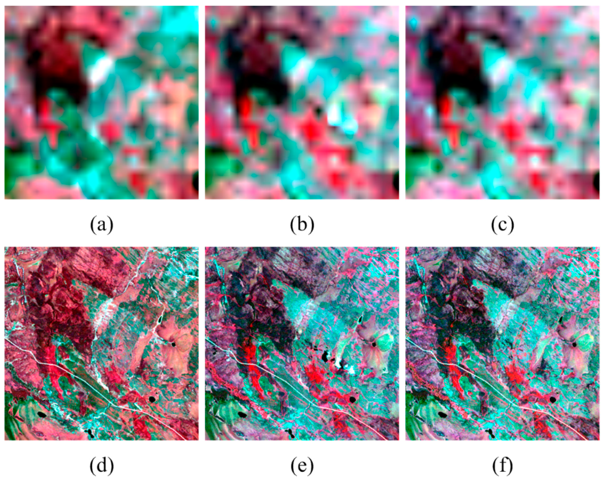Figure 2 shows the images using NIR–red–green as red–green–blue composite for both the Landsat and simulated MODIS images. This study area has relatively simple land-cover distribution with large land-cover patches. Most temporal changes are due to phenology changes during the period.

Figure 2. Near-infrared (NIR)–green–blue composites of the simulated-MODIS imagery (upper row) and Landsat imagery (lower row) taken on (a,d) 24 May 2001, (b,e) 11 July 2001, and (c,f) 12 August 2001, respectively.

The Landsat image on 11 July 2001 is set as the target image for prediction. The other Landsat and simulated MODIS images are used as inputs for STARFM, ESTARFM, and our proposed STBDF-I and STBDF-II algorithms, respectively. The predicted high-resolution images are compared with the reference Landsat image to evaluate the performance of the algorithms.

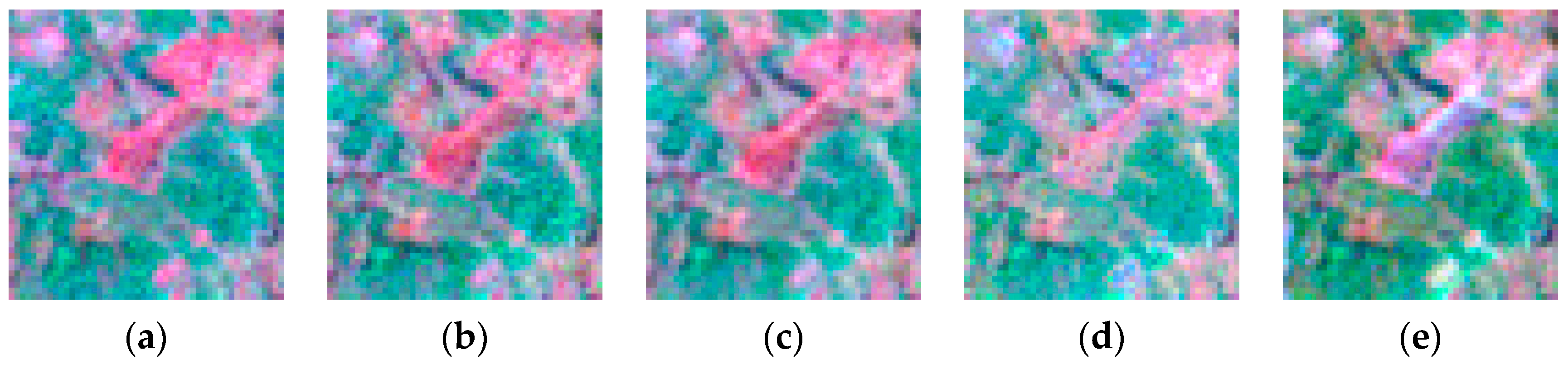
Figure 3 shows the reference image on 11 July 2001 and the predicted ones by STARFM, ESTARFM, STBDF-I, and STBDF-II, respectively. It is clear that all four algorithms have good performance in capturing the main reflectance changes over time. STARFM performs almost equally well with ESTARFM. STBDF-I and -II are better in capturing the reflectance changes and fine spatial details of small parcels, and in identifying objects with sharp edges and bright colors. The images predicted by STBDF-I and -II seem to be more similar to the reference image and maintain more spatial details than those obtained by STARFM and ESTARFM. Their differences are highlighted in the zoomed-in images shown in Figure 4. Clear shapes and distinct textures can be found in the results of our algorithms (Figure 4b,c), while the shapes are blurry and some spatial details are missing in the results of STARFM and ESTARFM (Figure 4d,e); the shapes are even difficult to identify in Figure 4d. For the second set of the zoomed-in images (Figure 4f–j), the color of the images obtained from our algorithms (Figure 4g,h) are closer to the reference image (Figure 4f) than the results of STARFM and ESTARFM (Figure 4i,j), respectively, which are distorted. The red color in the result of STARFM (Figure 4i) turns out to be a little bit pink and the green color in the result of ESTARFM (Figure 4j) looks greener than in the reference image (Figure 4f).

Figure 3. The (a) actual image acquired on 11 July 2001 and its predictions by (b) STBDF-I (Spatio-Temporal Bayesian Data Fusion I), (c) STBDF-II, (d) STARFM (Spatial and Temporal Adaptive Reflectance Fusion Model), and (e) ESTARFM (enhanced STARFM).

Figure 4. Zoomed-in images of the upper-right box (top row) and lower-left box (bottom row) marked in Figure 3a corresponding to the images in Figure 3a–e.

In order to quantitatively evaluate these approaches, AAD, RMSE, CC, and ERGAS are computed and shown in Table 2 for the three bands. The values of AAD, RMSE, and CC are comparable between STARFM and ESTARFM. For the green band, STARFM performs slightly better than ESTARFM, while for red and NIR bands, ESTARFM shows better performance. In terms of ERGAS, which evaluates the overall performance by putting the three bands together, the prediction error of ESTARFM is smaller than that of STARFM, in agreement with [9]. In comparison, our proposed STBDF-I and -II both exhibit improved prediction than STARFM and ESTARFM in terms of the three bands and the four metrics. Especially, STBDF-II outperforms STBDF-I, implying that adding information from the high-frequency image of the nearest Landsat images is capable of enhancing the fusion result. In summary, the predicted Landsat images obtained from STBDF-I and -II show better performance compared to the reference image than those from STARFM and ESTARFM, and STBDF-II gives the most accurate result in terms of both visual analysis and quantitative assessment.

Table 2. Quantitative metrics of the fusion results of the simulated images.

	AAD			RMSE			CC			ERGAS
Approaches	Green	Red	NIR	Green	Red	NIR	Green	Red	NIR	Overall
STARFM	0.0033	0.0038	0.0111	0.0084	0.0088	0.0182	0.6679	0.7513	0.9001	1.0551
ESTARFM	0.0038	0.0037	0.0111	0.0086	0.0085	0.0164	0.6670	0.7705	0.9252	1.0312
STBDF-I	0.0032	0.0037	0.0089	0.0077	0.0083	0.0143	0.7344	0.7867	0.9382	0.9718
STBDF-II	0.0029	0.0034	0.0089	0.0075	0.0081	0.0143	0.7475	0.7995	0.9386	0.9461

AAD, Average Absolute Difference; RMSE, Root-Mean-Square Error; CC, Correlation Coefficient; ERGAS, Erreur Relative Globale Adimensionnelle de Synthèse.

4.3. Test with Satellite Images

It is difficult to eliminate the influence of mismatching factors such as bandwidth, acquisition time, and geometric inconsistencies between two different sensors (i.e., Landsat and MODIS). With these in mind, we construct two test cases using real MODIS images. Since STBDF-II outperforms STBDF-I in the test using simulated MODIS images, we focus on STBDF-II in the following two tests. The first test employs the data source same as the test discussed in the previous subsection while the second test focuses on the Panyu area of Guangzhou city in China, where the landscape has more heterogeneous characteristics and small patches, which generally results in more mixed pixels in the MODIS images [9].

4.3.1. Experiment on a Homogeneous Region

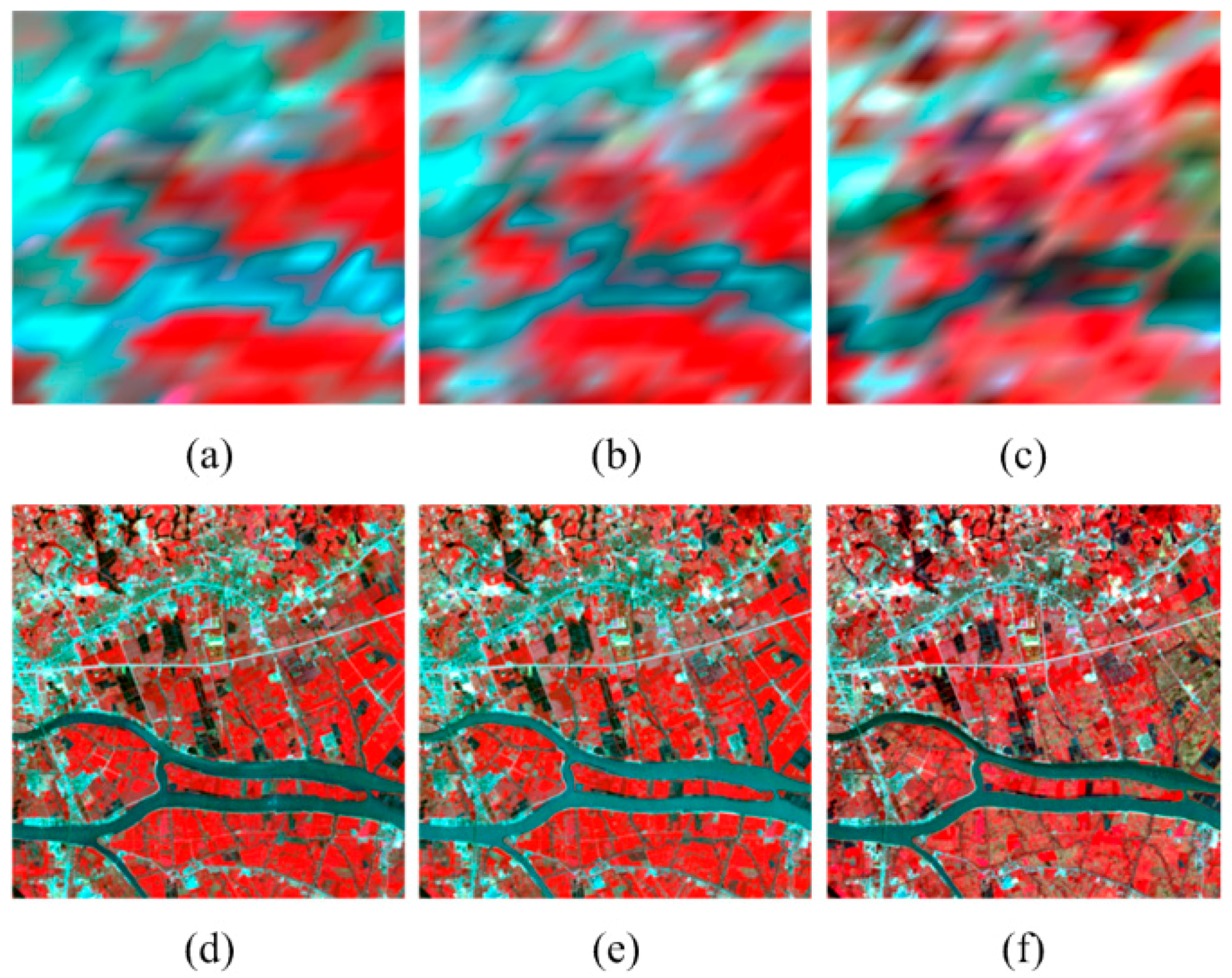
In this experiment, we use the same data source as the previous test. The difference is that we employ three real Landsat–MODIS image-pairs acquired on 24 May, 11 July, and 12 August in 2001, respectively. Another difference from the previous test is that we use a subset of 800 × 800 pixels from the original images in [5]. We focus on three bands: green, red, and NIR. The NIR–red–green composites of both Landsat and MODIS images are shown in Figure 5. Similar to the previous test, the objective here is to predict the high-resolution image on 11 July 2001 using all other images as inputs.

Figure 5. NIR–green–blue composites of the MODIS imagery (upper row) and Landsat imagery (lower row) taken on (a,d) 24 May 2001, (b,e) 11 July 2001, and (c,f) 12 August 2001, respectively.

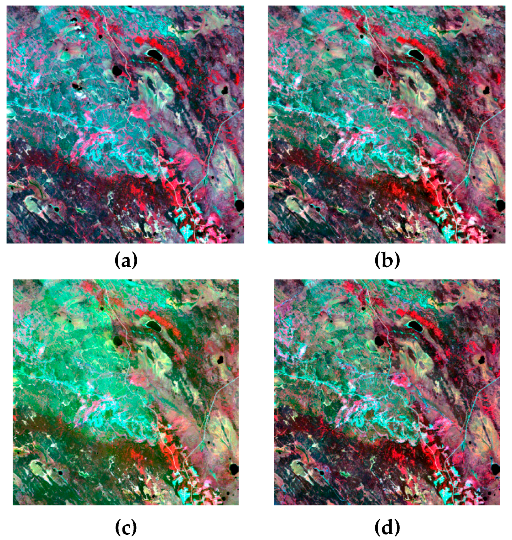
In this experiment, we employed STARFM, ESTARFM, and STBDF-II to predict the target Landsat image on 11 July 2001. As shown in Figure 6, all fused images obtained from the three algorithms capture the main spatial pattern and subtle details of the reference Landsat image. The upper-left portion of the predicted image from STARFM seems to have some color distortion, which is greener than in the three other images. This may be due to the relatively poorer performance of STARFM in predicting the red band than the other two methods, consistent with the quantitative results shown in Table 3. The results obtained by STBDF-II are similar to ESTARFM in both color and spatial details. 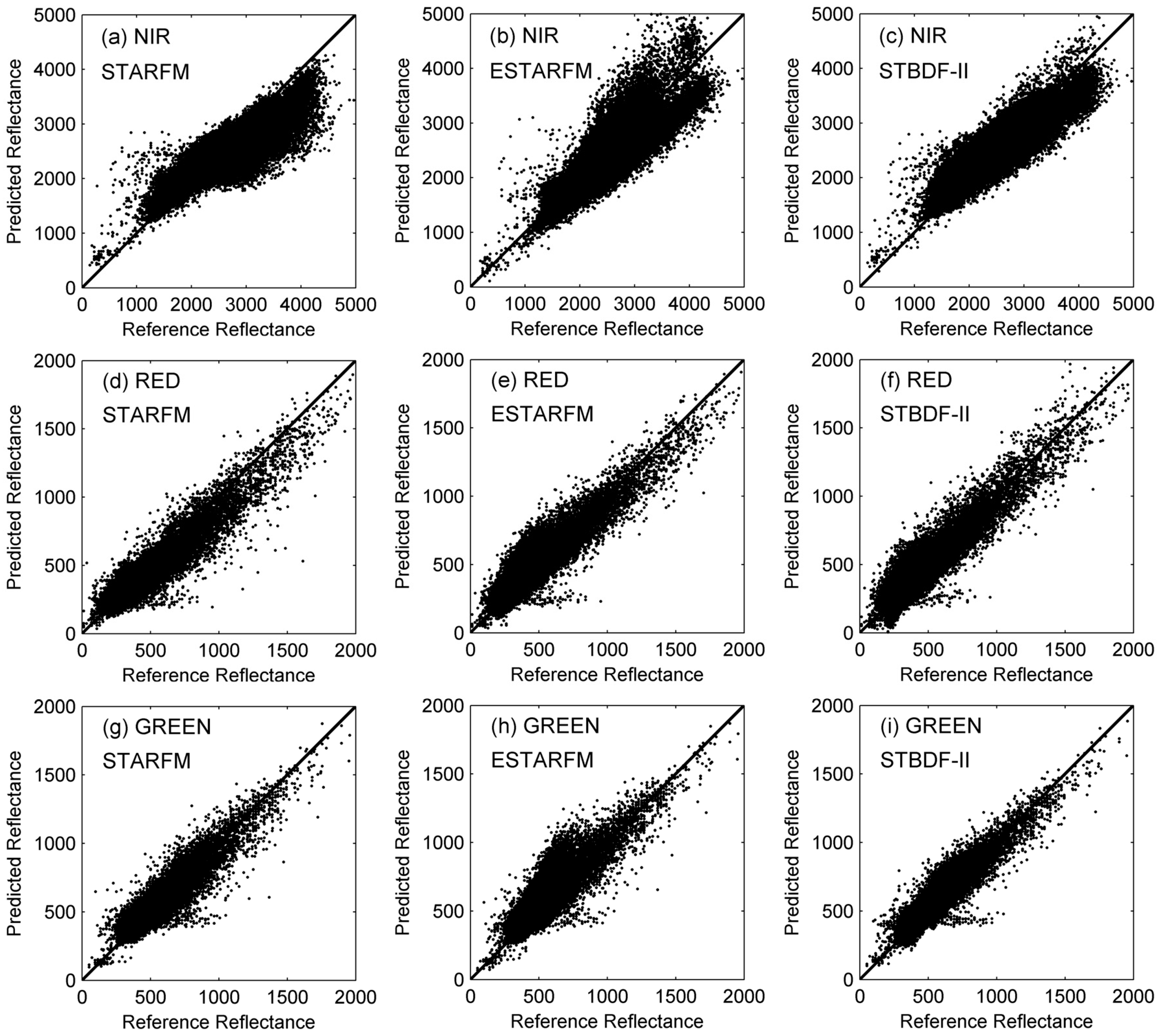Figure 7 shows the scatter plots of the predicted reflectance against the reference reflectance for each pixel in the NIR, red, and green bands, respectively. In terms of NIR and green bands, it appears that the points from STARFM and ESTARFM are more scattered, while those from STBDF-II are closer to the 1:1 line. For the red band, ESTARFM seems to produce better scatter plots than STARFM and our STBDF-II method. These results are consistent with the quantitative assessment results shown in Table 3. In terms of the synthetic metric ERGAS, STBDF-II (1.0196) outperforms STARFM (1.1493) and ESTARFM (1.0439).

Figure 6. The (a) actual image acquired on 11 July 2001 and its predictions by (b) STBDF-II; (c) STARFM; and (d) ESTARFM.

Table 3. Quantitative metrics of the fusion results applied to the Boreal images.

	AAD			RMSE			CC			ERGAS
Approaches	Green	Red	NIR	Green	Red	NIR	Green	Red	NIR	Overall
STARFM	0.0036	0.0044	0.0133	0.0076	0.0099	0.0207	0.7818	0.7700	0.9102	1.1493
ESTARFM	0.0041	0.0040	0.0159	0.0081	0.0081	0.0226	0.7575	0.8439	0.8913	1.0439
STBDF-II	0.0035	0.0043	0.0132	0.0075	0.0084	0.0191	0.7939	0.8340	0.9216	1.0196

Figure 7. Scatter plots of the predicted reflectance against the actual reflectance. (a–c) Scatter plots of the predicted reflectance using STARFM, ESTARFM, and STBDF-II against the actual reflectance in the NIR band, respectively; (d–f) the red band; (g–i) the green band.

4.3.2. Experiment on a Heterogeneous Region

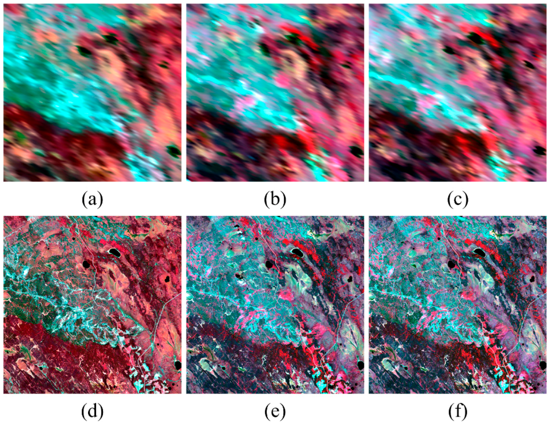
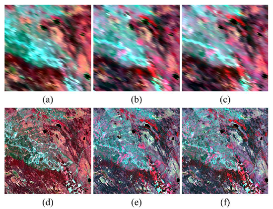
In this experiment, our satellite images were acquired over the Panyu area in Guangzhou, China. Panyu is an important area for crop production in the Pearl River Delta with complex land-cover types, including cropland, farmland, forest, bare soil, urban land, and water body. In this area, Landsat-7 ETM+ images (30 m) with 300 × 300 pixels and MODS images (1000 m) over the same region were acquired on 29 August 2000, 13 September 2000, and 1 November 2000, respectively (Figure 8). 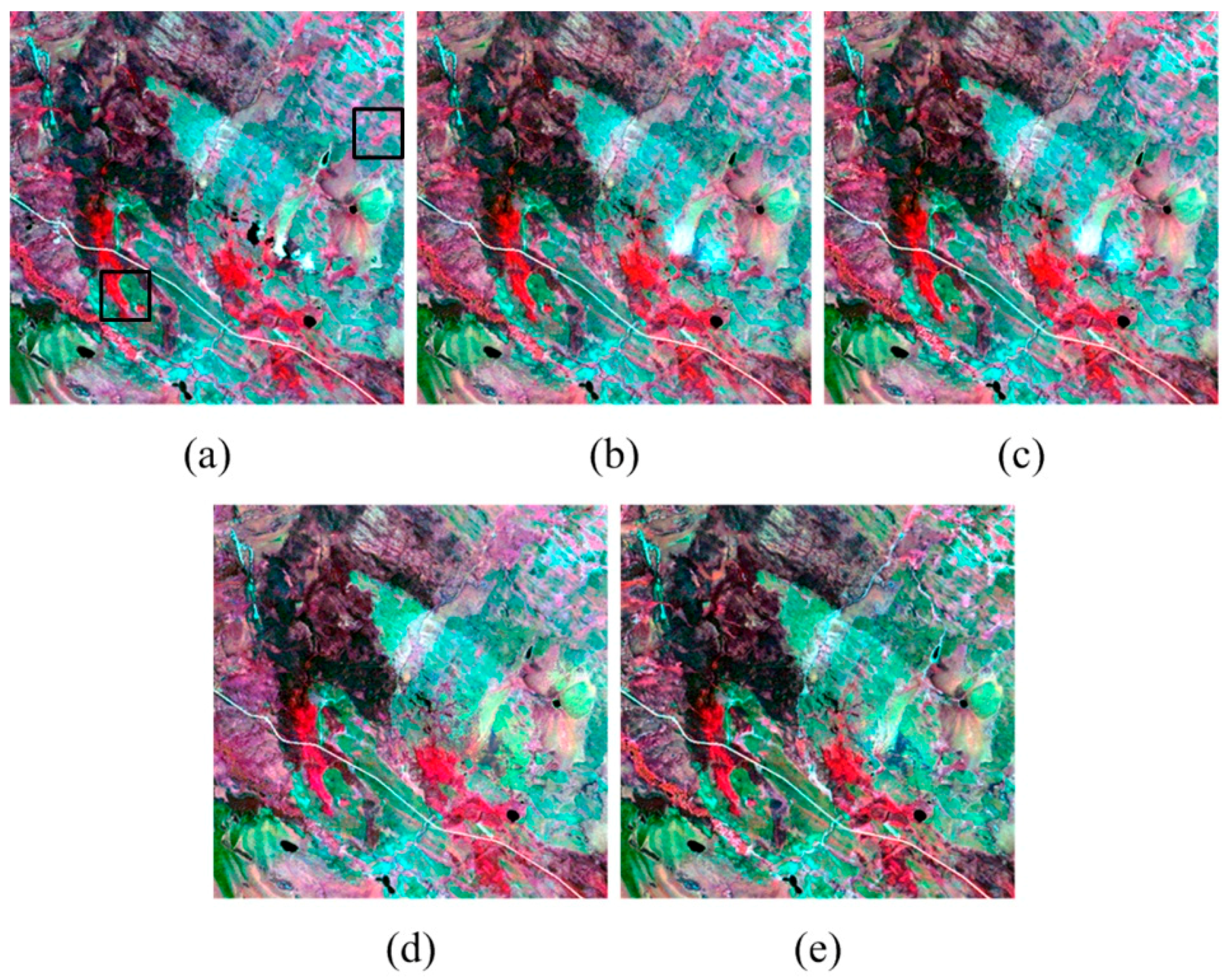Changes in the vegetation phenology are clearly observed in the Landsat images from 13 September to 1 November 2000 (Figure 8e,f). The high-resolution image on 13 September 2000 is targeted for prediction. All five other images are used as inputs for STARFM, ESTARFM, and STBDF-II, respectively.

Figure 8. NIR–green–blue composites of MODIS imagery (upper row) and Landsat imagery (lower row) taken on (a,d) 29 August 2000, (b,e) 13 September 2000, and (c,f) 1 November 2000, respectively.

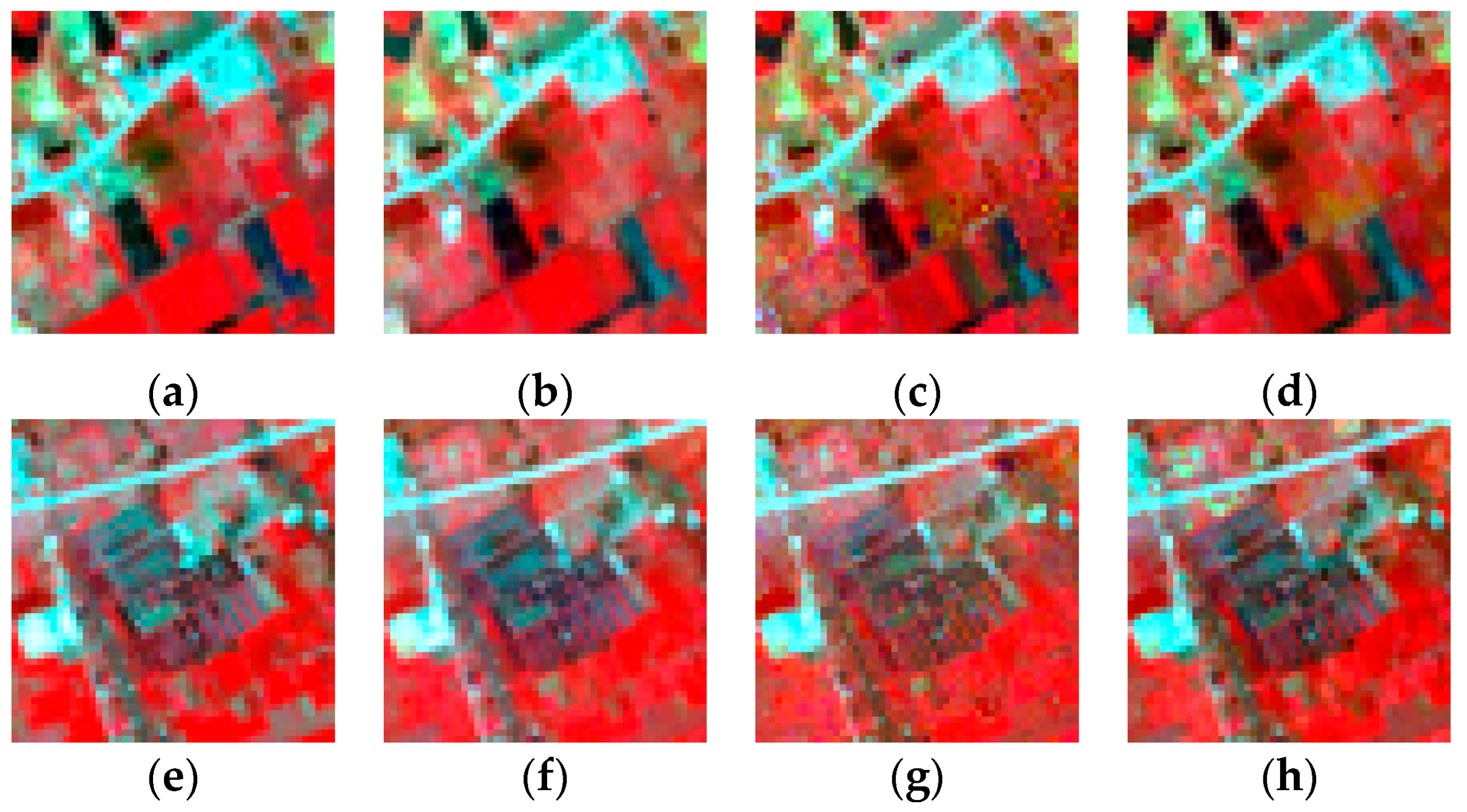
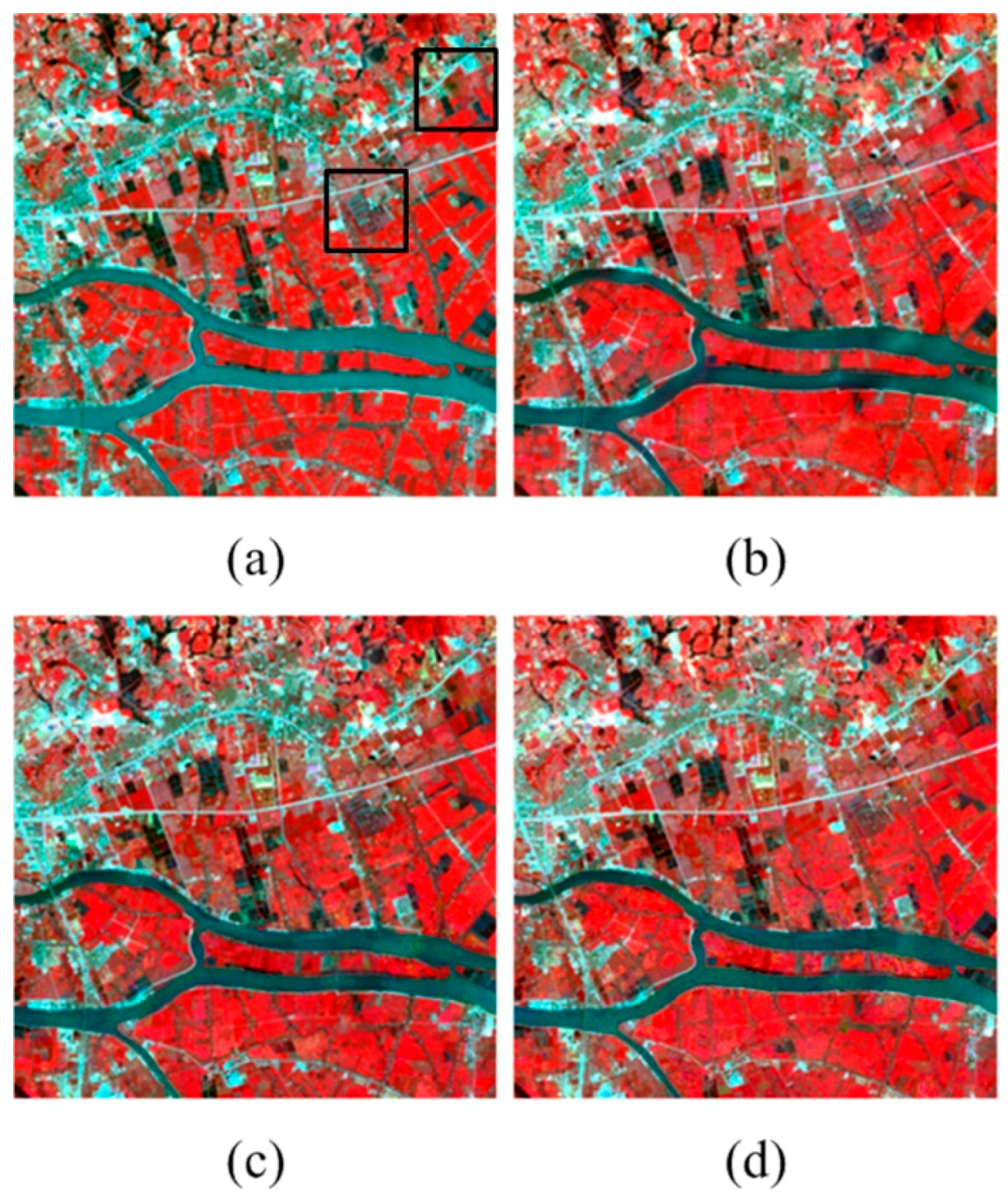
Figure 9 depicts the reference Landsat image and the three predicted images from STARFM, ESTARFM, and STBDF-II, respectively. The three algorithms are all capable of predicting the target image by capturing many spatial details. It appears that colors of the image predicted by STBDF-II are visually more similar to the reference image in terms of better hue and saturation than those by STARFM and ESTARFM. Moreover, STBDF-II captures almost all the spatial details and fine textures in the reference image, while STARFM and ESTARFM fail to maintain some details. To highlight the visual difference in Figure 9, we give two sets of zoomed-in images as illustrated in Figure 10 with respect to the two black boxes shown in Figure 9. As shown in the first set of the zoomed-in images (Figure 10a–d), the colors and the shapes of vegetation patches in the image generated by STBDF-II (Figure 10b) is closer to the reference image (Figure 10a) than those by STARFM and ESTARFM (Figure 10c,d). Some pixels produced by STARFM and ESTARFM seem to have abnormal values, leading to a visually brown color in several patches. From the second set of the zoomed-in images (Figure 10e–h), it is clear that the shapes of the buildings predicted by STBDF-II (Figure 10f) are more similar to those in the reference image (Figure 10e). The buildings (in blue color) in the middle of the predicted images by STARFM and ESTARFM (Figure 10g,h) seem to lose some spatial details and shapes with blurry boundaries. 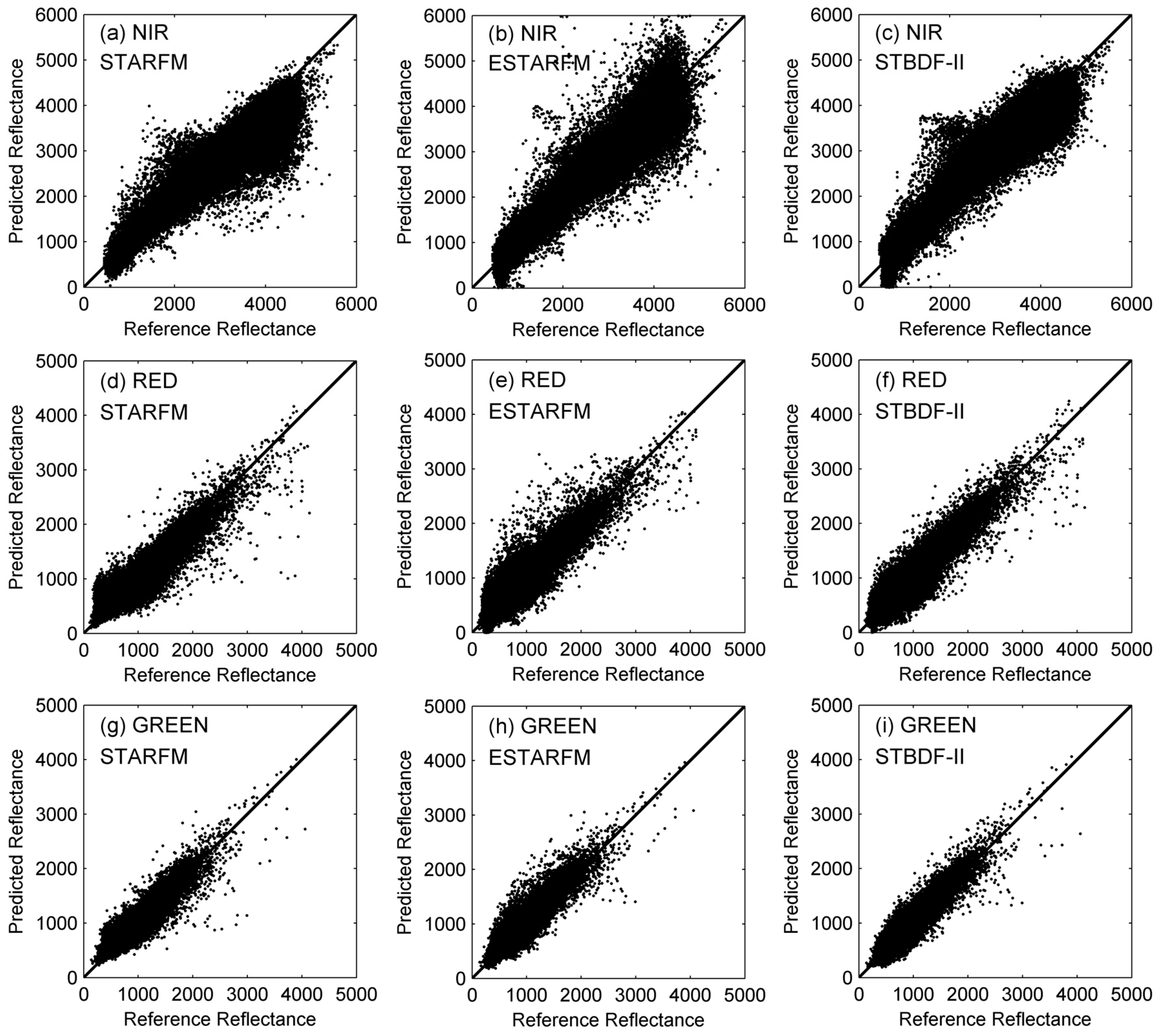Figure 11 shows the scatter plots of the predicted reflectance against the reference reflectance in the NIR, red, and green bands, respectively. Results of the quantitative measures are summarized in Table 4. STBDF-II achieves the best results, except for the AAD and RMSE values for the red band that are, however, very close to those of the other two algorithms (STARFM produces a slightly better result). Nevertheless, the ERGAS values in Table 4 indicate that the fusion quality of STBDF-II outperforms those of STARFM and ESTARFM from a synthetic perspective.

Figure 9. The (a) actual image acquired on 13 September 2000 and its predictions by (b) STBDF-II, (c) STARFM, and (d) ESTARFM.

Figure 10. Zoomed-in images of the upper-right box (top row) and lower-left box (bottom row) marked in Figure 10a corresponding to the images in Figure 10a–d.

Figure 11. Scatter plots of the predicted reflectance against the actual reflectance. (a–c) Scatter plots of the predicted reflectance using STARFM, ESTARFM, and STBDF-II against the actual reflectance in the NIR band, respectively; (d–f) the red band; (g–i) the green band.

Table 4. Quantitative metrics of the fusion results applied to the Panyu images.

	AAD			RMSE			CC			ERGAS
Approaches	Green	Red	NIR	Green	Red	NIR	Green	Red	NIR	Overall
STARFM	0.0109	0.0130	0.0267	0.0140	0.0204	0.0383	0.9057	0.8998	0.9376	1.1442
ESTARFM	0.0104	0.0130	0.0244	0.0136	0.0205	0.0347	0.9157	0.8997	0.9420	1.1220
STBDF-II	0.0104	0.0140	0.0243	0.0133	0.0205	0.0333	0.9208	0.9049	0.9443	1.1087

5. Discussion

The fusion results with simulated data demonstrated that our methods are more accurate than both STARFM and ESTARFM, and that STBDF-II outperforms STBDF-I. The improved performance of STBDF-II over STBDF-I highlights the importance of incorporating more temporal information for parameter estimation. The better performance of STBDF-II over STARFM and ESTARFM is shown in another two tests using acquired real Landsat–MODIS image pairs. STARFM is specifically developed for homogeneous landscapes, while STBDF-II, to some extent, incorporates sub-pixel heterogeneity into fusion process through the employment of high frequencies of high-resolution images, which may partly explain the outperformance of our algorithm over STARFM. ESTARFM assumes a linear trend for temporal changes, which does not hold for the three bands in terms of mean reflectance. However, this nonlinear change is well captured by STBDF-II (not shown), which may be partly due to the use of joint Gaussian distribution in our algorithm to simulate temporal evolution of the image series. Though the improvement of our approach over ESTARFM is not as significant as it is over STARFM, the advantage of our approach over ESTARFM is that we impose no requirements on the number of input image pairs, and it can work on one input image pair. ESTARFM can only fuse images based on two input image pairs.

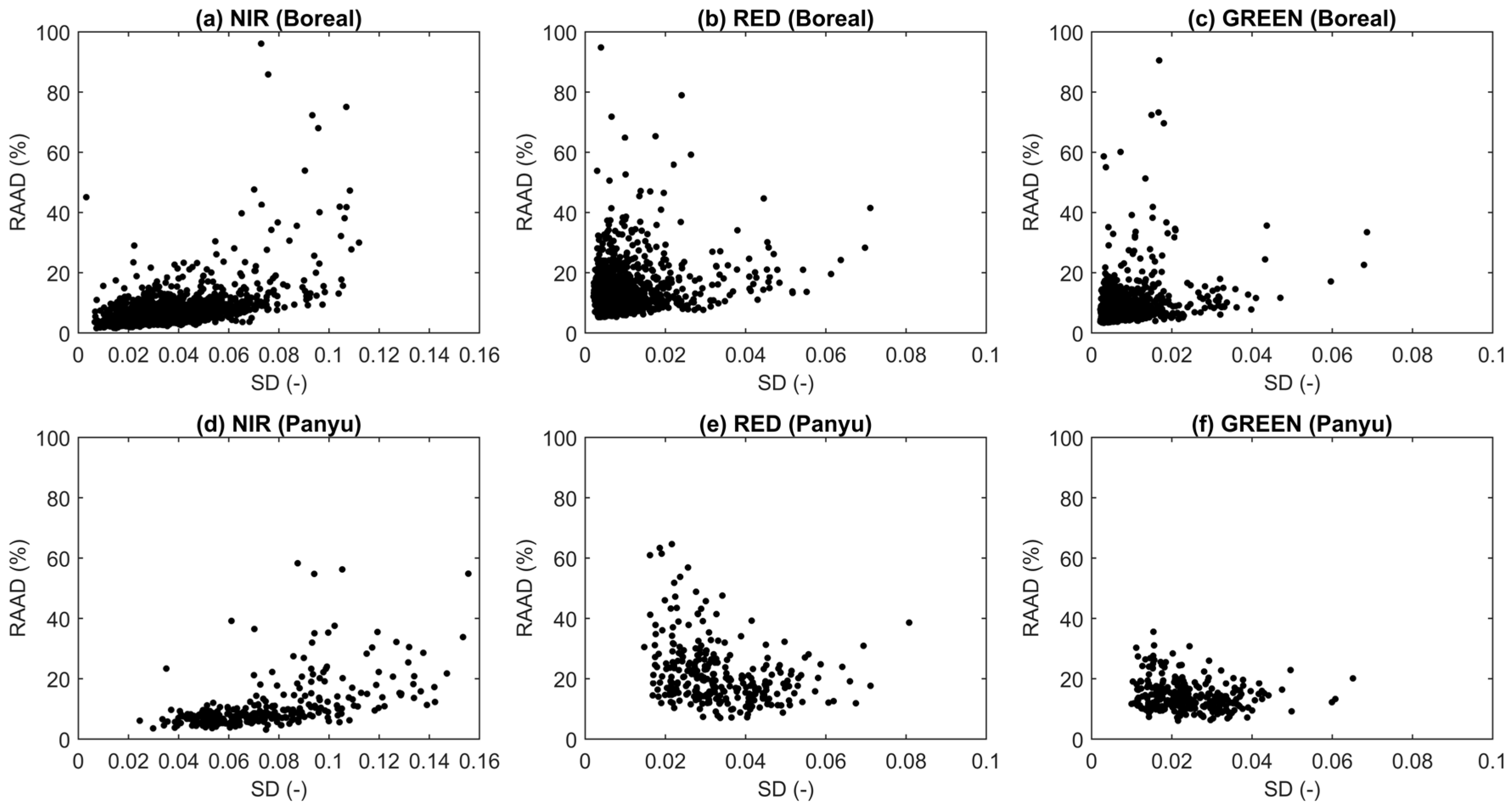
Our study employed two datasets with different landscape heterogeneities to understand the utility of our algorithm. Following the results section, here we provide more discussions on this issue. To objectively define the sub-pixel heterogeneity, we compute the standard deviation (SD) of reflectance for Landsat pixels within each MODIS pixel. High SD indicates high heterogeneity. Within each MODIS pixel, we can also compute relative average absolute difference (RAAD) to represent the bias of the predicted Landsat image relative to the reference Landsat image. The changing trend of RAAD with respect to SD would shed light on the impact of heterogeneity on the performance of our algorithm at MODIS pixel scales (Figure 12). Reasonably, we observe that the homogeneous Boreal data generally shows lower SD than the heterogeneous Panyu data. In red and green bands, SDs are well concentrated below 0.2 for Boreal data, while most pixels in Panyu data have SDs larger than 0.2. In the NIR band, SDs approximately range from 0 to 0.1 for Boreal data, and from 0.02 to 0.14 for Panyu data. For the two datasets with different heterogeneities, the RAAD of most pixels from the three bands is well constrained at low values, suggesting the skill of our algorithm for landscapes with different complexities. Another interesting aspect is that the lower boundary of RAAD generally shows a slowly increasing trend with respect to SD, suggesting that increased heterogeneity would increase the difficulty of accurate fusion. However, the trend of increase is quite flat (Figure 12). The varying upper boundary may indicate the impacts from other factors.

Figure 12. Changes of relative average absolute difference (RAAD) with respect to standard deviation (SD) of reflectance from Landsat pixels within each MODIS pixel for (a–c) Boreal data and (d–f) Panyu data.

The assumptions for estimating the mean vector and covariance matrix of the joint Gaussian distribution of the high-resolution image series may have impact on the fusion accuracy. Here we conduct several experiments to explore this impact quantitatively in terms of CC and ERGAS. For the mean estimate, we assume the target high-resolution image is available and add the high frequencies of it to the interpolated low-resolution image to estimate the mean vector, which is named as case ideal-I. For the covariance estimate, we assign the target high-resolution image instead of the interpolated low-resolution image to clusters to estimate the covariance, named case ideal-II. We use Panyu dataset as an example. Results from the two cases are compared with the control case in which the assumptions are not relaxed, respectively (Table 5 and Table 6). As shown in Table 5, the use of high frequencies from target image for mean vector estimates improves the fusion results in terms of CC and ERGAS, especially for green and red bands. However, we do not find the significant improvements through the use of reference high-resolution image for covariance estimation (Table 6). These results suggest that the fusion accuracy is more sensitive to approximations in mean estimates than in covariance estimates. It should be noted that the mean has a much higher contribution than that of the covariance to the fused image, which may partly explain the sensitivity we see.

Table 5. CC and ERGAS of the fusion results applied to the Panyu images for both control and Ideal-I cases.

	CC			ERGAS
Approaches	Green	Red	NIR	Overall
Control	0.9208	0.9049	0.9443	1.1087
Ideal-I	0.9776	0.9750	0.9740	0.6764

Table 6. CC and ERGAS of the fusion results applied to the Panyu images for both control and Ideal-II cases.

	CC			ERGAS
Approaches	Green	Red	NIR	Overall
Control	0.9208	0.9049	0.9443	1.1087
Ideal-II	0.9208	0.9047	0.9445	1.1085

Although the proposed Bayesian approach enhances our capability in generating remotely sensed images high in both spatial and temporal resolutions, there are still limitations and constraints that need further study. Firstly, the factors related to different sensors (i.e., different acquisition times, bandwidths, spectral response functions, etc.) and the model assumptions (i.e., rectangular PSF, joint Gaussian distribution, etc.) may affect the accuracy of fusion results. Secondly, we have not considered the hyperparameter prior information of the targeted high-resolution image, which might need to be taken into consideration in future studies. Thirdly, our approach, as well as STARFM and ESTARFM, have not fully incorporated the mixed-class spectra within a low-resolution pixel, which might limit its potential to retrieve the accurate class spectra in high resolution on the target date. Thus, we will combine the unmixing method together with the proposed Bayesian approach in a unified way in the future. Finally, the proposed framework can be extended to incorporate time series of low-resolution images in the fusion process. This will be considered in future studies.

6. Conclusions

In this study, we have developed a Bayesian framework for the fusion of multi-scale remotely sensed images to obtain images high in both spatial and temporal resolutions. We treat fusion as an estimation problem in which the fused image is estimated by first constructing a first-order observational model between the target high-resolution image and the corresponding low-resolution image, and then by incorporating the information of the temporal evolution of images into a joint Gaussian distribution. The Bayesian estimator provides a systematic way to solve the estimation problem by maximizing the posterior probability conditioned on all other available images. Based on this approach, we have proposed two algorithms, namely STBDF-I and STBDF-II. STBDF-II is an improved version of STBDF-I through the incorporation of more information from the high-frequency images of the high-resolution images nearest to the target image to produce better mean estimates.

We have tested the proposed approaches with an experiment using simulated data and two experiments using acquired real Landsat–MODIS image pairs. Through the comparison with two widely used fusion algorithms STARFM and ESTARFM, our algorithms show better performance based on visual analysis and quantitative metrics, especially for NIR and green bands. In terms of a comprehensive metric ERGAS, STBDF-II improves the fused images by approximately 3–11% over STARFM and approximately 1–8% over ESTARFM for the three experiments.

In summary, we have proposed a formal and flexible Bayesian framework for satellite image fusion which gives spatio-temporal fusion of remotely sensed images a solid theoretical and empirical foundation on which rigorous statistical procedures and tests can be formulated for estimations and assessments. It imposes no limitations on the number of input high-resolution images and can generate images high in both spatial and temporal resolutions, regardless of over-homogeneous or relatively heterogeneous areas.