Non-Cooperative Bistatic SAR Clock Drift Compensation for Tomographic Acquisitions

Abstract

In the last years, an important amount of research has been headed towards the measurement of above-ground forest biomass with polarimetric Synthetic Aperture Radar (SAR) tomography techniques. This has motivated the proposal of future bistatic SAR missions, like the recent non-cooperative SAOCOM-CS and PARSIFAL from CONAE and ESA. It is well known that the quality of SAR tomography is directly related to the phase accuracy of the interferometer that, in the case of non-cooperative systems, can be particularly affected by the relative drift between onboard clocks. In this letter, we provide insight on the impact of the clock drift error on bistatic interferometry, as well as propose a correction algorithm to compensate its effect. The accuracy of the compensation is tested on simulated acquisitions over volumetric targets, estimating the final impact on tomographic profiles.

1. Introduction

SAR tomography provides the capability of resolving the vertical structure of a volumetric target based on multibaseline acquisitions [1]. Since its early introduction, it has become a widely used tool for the study of the forests’ structures [2] with the linking of above-ground biomass (AGB) to the backscatter intensity derived from polarimetric tomographic profiles [3].

One limitation of using multibaseline acquisitions is the change of the target’s scattering elements in the case of significant temporal gaps between datatakes. This produces a coherence degradation between images that has a direct impact on the quality of the derived tomograms. This limitation can be overcome by performing single-pass (bistatic) interferometric acquisitions, for which a number of L-band missions have been proposed such as Tandem-L [4] and the recent non-cooperative SAOCOM-CS [5] and PARSIFAL from CONAE and ESA. The two latter can be regarded as “low-cost” solutions, which are implemented by placing a small, passive (receive-only) companion satellite (CS) orbiting in formation with an already developed active satellite [6,7].

A different challenge is presented with bistatic non-cooperative SAR interferometers, which is the accurate synchronization of their onboard clocks. Accurate synchronization is necessary for obtaining a common timeframe for referencing the bistatic SAR images, as well as for demodulating the passive received signal with the same central frequency that was used during transmission. Even with a perfect initial synchronization, small deviations from their nominal frequencies throughout an acquisition can introduce significant phase artifacts [8].

Cooperative missions specifically designed for bistatic operations, such as TanDEM-X, have tackled this issue by installing synchronization links on each platform [9]. However, in the case of companion-based systems, it is expected that the synchronization link can be dismissed and the corrections be estimated from the acquired SAR data (often known as autonomous calibration) as long as the signal can be acquired simultaneously [10]. This has the advantage of simplifying the system design, lowering costs, and potentially using the companion with any already-deployed SAR satellite, independently of whether it has or has not been foreseen for bistatic operations.

In this work, we present a method to estimate and compensate the clock drift perturbation from the interferometric phase without the need for dedicated synchronization links, i.e., by performing the estimation from the bistatic SAR images. Similar to the methods reported in References [10,11,12], a multisquint processing of the images is performed from which an estimation of the clocks’ drift function is obtained. In our method, however, we use a system inversion approach to directly estimate the clock drift function instead of its derivative, which eliminates the last integration step. The performance of the method is evaluated by assessing the calibration accuracy on simulated bistatic image pairs, as well as on tomographic profiles obtained from the calibrated image pairs.

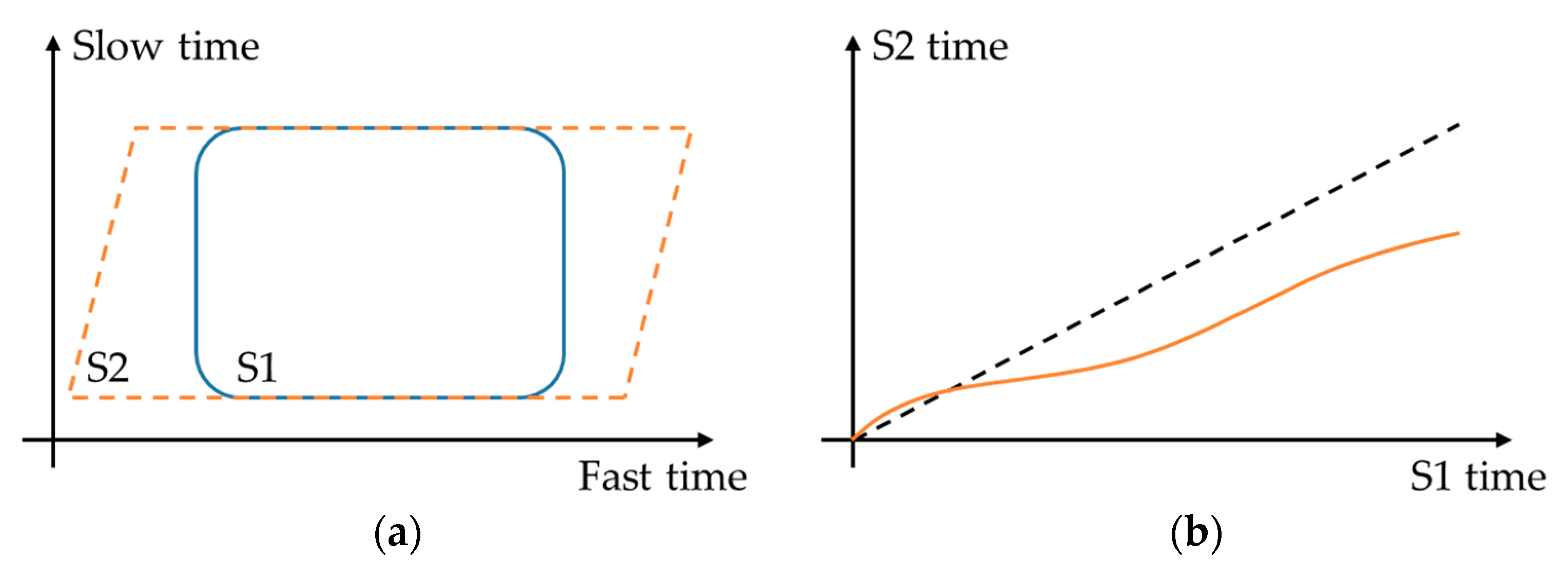
2. Clock Synchronization Problem

The absence of a synchronization link between platforms will mostly be an issue common to all future companion-based missions, in which a passive satellite is aggregated to orbit in formation with an existing active satellite, often designed and constructed independently from the former. This limitation poses two major problems (see Figure 1):

Figure 1. Schematic representation of synchronization problems. (a) Reception windows for the active satellite S1 (solid) and the passive S2 (dashed), for the case that it is contained inside S1. The skewness of the S2 window represents the frequency offset between oscillators. (b) The clock fluctuation between S1 and S2 is shown, with the ideal case S2 = S1 represented by the dashed line.

• Reception window synchronization: the reception window of the passive receptor must contain that of the active satellite during the whole acquisition, in order to avoid missing pulses.
• Phase synchronization: throughout an acquisition, the clock fluctuations between different onboard clocks must be bounded in order to allow proper focusing of the passive receiver image and avoid coherence loss between bistatic images.

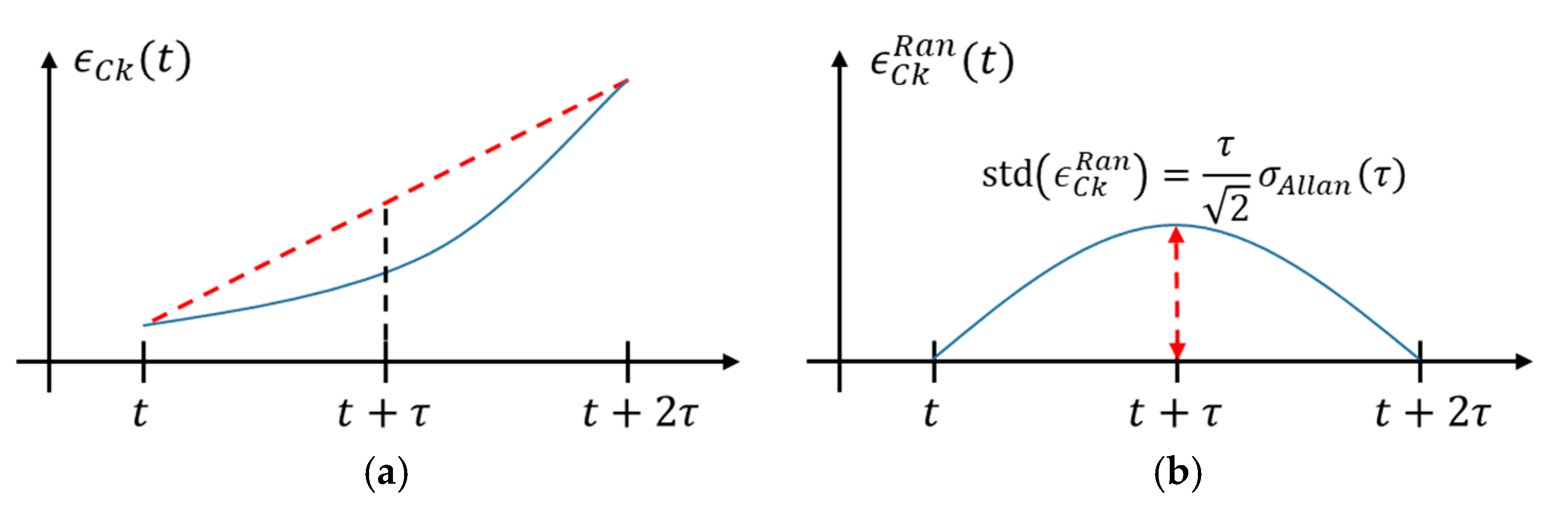
The first problem is the least restrictive, since the reception window can be coarsely synchronized as long as the acquisition remains valid (i.e., no pulses lost). The start of the acquisition is triggered by each satellite (e.g., by using Global Positioning System time), after which the timeline is kept by the local clocks carried on each platform. The time offset between windows is given by the triggering time uncertainty, while the skewness of the window is given by the frequency offset between oscillators.

A number of alternatives have been proposed to overcome this issue, the simplest being to lengthen the reception window of the passive receiver a sufficient amount [11]. Posterior corrections can include the application of autofocus techniques (Phase-Gradient Autofocus, contrast maximization) and incoherent correlation between monostatic and bistatic images in order to recover the coarse time and frequency offsets [11,12].

The second problem is the main interest of this work: even if the start of the acquisition is perfectly synchronized between satellites, with both oscillators running at the exact same frequency, clocks fluctuations throughout the acquisition can be important enough to cause significant phase artifacts. As an example, for SAOCOM-CS, acquisitions are foreseen to last up to 6 min, without chances of performing onboard corrections in between [1]. In this case, the error depends upon the stable local oscillator (STALO) stability, which is described in the following subsection.

Clock Stability

The clock drift error ${ϵ}_{Ck}\left(t\right)$ is defined as the difference between the clocks’ timekeeping. It can be decomposed as a linear component (frequency offset) plus a random component ${ϵ}_{Ck}^{Ran}\left(t\right)$ [13], shown schematically in Figure 2. The linear component is unbounded and increases—in probabilistic terms—with the elapsed time since the last oscillators’ synchronization. The random component, on the other hand, is independent of the elapsed time and bounded by the so-called Allan deviation of the oscillator, ${\sigma }_{Allan}$, which characterizes the expected oscillator’s frequency fluctuation within a certain period [14].

Figure 2. Clock drift error ${ϵ}_{Ck}\left(t\right)$ is shown schematically: (a) along with its linear component represented by dashed line and (b) with its linear component subtracted, yielding the random component ${ϵ}_{Ck}^{Ran}\left(t\right)$, which has a maximum deviation within a time interval $\mathrm{\Delta }t=2\tau$ bounded by $std\left({ϵ}_{Ck}^{Ran}\right)=\frac{\tau }{\sqrt{2}}{\sigma }_{Allan}\left(\tau \right)$.

Assuming both STALOs with the same Allan deviation, the clock drift random component ${ϵ}_{Ck}^{Ran}\left(t\right)$ is bounded as follows:

$$std\left({ϵ}_{Ck}^{Ran}\left(t+\tau \right)\right)=\tau {\sigma }_{Allan}\left(\tau \right).$$

(1)

Note that this expression is dependent only on the elapsed time $\tau$, not on the absolute time $t$. This allows putting a bound on the oscillator’s stability in order to focus an image properly. Taking as a reference the synthetic aperture time for SAOCOM, with its antenna length $L_{\mathrm{x}}=10 \mathrm{m}$, it yields:

$${\tau }_{syn}=\frac{\lambda r}{L_{\mathrm{x}}v}\approx 2 \mathrm{s}.$$

(2)

$\lambda$ is the SAR wavelength and $r$ the slant range distance. Posing as a requirement a phase error less than 5 degrees within the synthetic aperture time, we obtain the oscillator’s stability requirement:

$${\sigma }_{Allan}\left(\tau =1s\right)<5\mathrm{E}-12\mathrm{s}.$$

(3)

Modern space-qualified STALOs can reach stabilities in the order of 1E-12 or better [15]. Hence, the clock stability will usually not be an issue for focusing the passive receiver image if a sufficiently precise oscillator is used. However, low-frequency phase artifacts can become appreciable in the interferometric phase for long acquisitions. As an example, oscillators with an Allan deviation of 1E-12 may cause up to 60 degrees of random phase error at the L-band during a 30-s acquisition, which justifies the need for compensation.

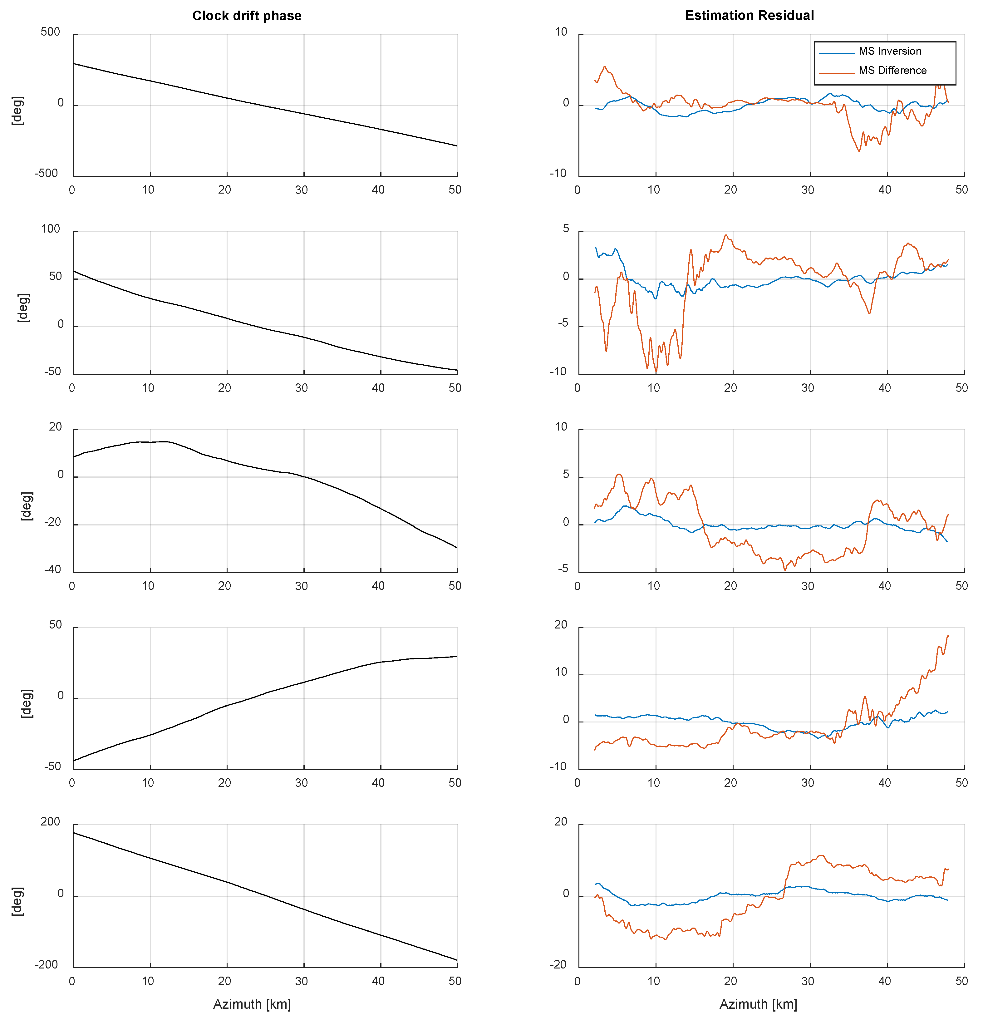
3. Phase Compensation Method

The proposed algorithm is based on separating the interferometric phase due to the clock drift from that due to the scene, which carries the actual information. Hence, it is assumed that the preliminary calibration procedure required to remove the coarse clock time and frequency offsets (see Section 2) has already been applied to the images.

Each bistatic image pair is calibrated independently. This is due to the fact that acquisitions performed over forest regions on different dates are expected to decorrelate almost completely, due to the long spaceborne revisit times. For tomographic imaging, a quasi-monostatic acquisition geometry is assumed, which is characterized by short along-track and varying across-track baselines. The bistatic interferometric phase can be expressed as:

$${\varphi }_{BI}\left(x,r,\psi \right)={\varphi }_{SYS}\left(x-r\psi \right)+{\varphi }_{TOPO}\left(x,r\right)$$

(4)

where ${\varphi }_{SYS}$ represents the phase perturbations due to the system (clock and orbits) and ${\varphi }_{TOPO}$ is the phase from the illuminated scene, i.e., it carries the information about the ground scatterers and topography. Ionospheric effects are disregarded, since they can be removed with already existing techniques such as split spectrum [16]. In addition, if the ionospheric gradients are low enough, its effect on the interferometric phase can be compensated for by the quasi-monostatic geometry.

${\varphi }_{BI}$ depends on azimuth $x$, slant range $r$, and processed squint angle $\psi$. The latter is not the SAR antenna physical squint, but the central squint angle chosen for focusing the images. It is explicitly included because it allows for separating the topography from the system phases.

The topographic and system phase components are given as follows:

$${\varphi }_{TOPO}\left(x,r\right)=-\frac{2\pi }{\lambda }\frac{B_{\perp }}{r\sin \left(\theta \right)}{ϵ}_{DEM}\left(x,r\right)$$

(5)

$${\varphi }_{SYS}\left(x-r\psi \right)={\varphi }_{CLOCK}\left(x-r\psi \right)+{\varphi }_{ORBIT}\left(x-r\psi ,r\right)$$

(6)

$${\varphi }_{CLOCK}\left(x-r\psi \right)=2\pi f_0{ϵ}_{Ck}\left(x-\psi r\right)\left(1+\frac{1}{4}\frac{B_{\perp }}{r\tan \left(\theta \right)}\right).$$

(7)

${ϵ}_{DEM}$ is the topographic height uncertainty and $B_{\perp }$ is the perpendicular baseline. ${ϵ}_{Ck}$ is the clock drift error in (s). The right-hand side term inside the parenthesis of Equation (7) is a residual component caused by the slant range shift of the passive receiver signal that can often be neglected due to its inverse dependence with range.

In addition to this phase term, the clock drift causes a range time shift and its slope an azimuth shift on the passive receiver focused image as follows:

$$\mathrm{\Delta }{t}_{Az}\left(t\right)=\frac{rc}{2v^2}\frac{d{ϵ}_{Ck}\left(t\right)}{dt}$$

(8)

$$\mathrm{\Delta }{t}_{Rg}\left(t\right)={ϵ}_{Ck}\left(t\right).$$

(9)

$c$ is the speed of light and $v$ the platform velocity. In this model, the decorrelation introduced by $\mathrm{\Delta }{t}_{Az}$ and $\mathrm{\Delta }{t}_{Rg}$ is considered negligible. If this is not the case, a coarse calibration as described in Section 2 should be performed as a preliminary step in order to obtain a coherent interferogram.

From Equations (5) and (6), it can be observed that the topographic phase does not depend on squint, while the system phase has an $r\psi$ dependence. This allows for a separation between them by exploiting the multisquint interferograms, which is also the basis of the methods in References [17,18,19].

In order to isolate ${\varphi }_{SYS}$, we explore two methods:

• MultiSquint phase difference (MS Difference);
• MultiSquint Linear system inversion (MS Inversion).

The first method relies on the squint difference of the bistatic phase to eliminate the topographic component, which could be regarded as a special case of the autosync method [10,11,12]. Afterwards, an integration step recovers the desired phase:

$$\begin{array}{ccc}\mathrm{\Delta }{\varphi }_{BI}\left(x,r\right)& =& {\varphi }_{BI}\left(x,r,\mathrm{\Delta }\psi \right)-{\varphi }_{BI}\left(x,r,-\mathrm{\Delta }\psi \right)\\ & =& {\varphi }_{SYS}\left(x-r\mathrm{\Delta }\psi \right)-{\varphi }_{SYS}\left(x+r\mathrm{\Delta }\psi \right)\\ {\varphi }_{SYS}\left(x\right)& =& -{{\displaystyle \sum }}_{l=0}^x\frac{1}{2\mathrm{\Delta }\psi }⟨\mathrm{\Delta }{\varphi }_{BI}{\left(l,r\right)⟩}_r\frac{dl}{r}\end{array}.$$

(10)

$⟨\mathrm{\Delta }{\varphi }_{BI}{\left(l,r\right)⟩}_r$ is the bistatic phase difference evaluated at azimuth $l$, averaged along range, and $\pm \mathrm{\Delta }\psi$ is the squint span. This approach has the advantage of computational simplicity, since it can be implemented by processing only two sub-apertures. However, the final integration step is a drawback since it accumulates errors, making the estimation prone to trends and increased uncertainties with the integration length.

The second method expresses the bistatic interferometric phases as a linear system, subsequently retrieving each component with an ordinary least squares (OLS) inversion. This eliminates the need for the final integration step, thus providing robustness to the estimation. The drawback is that it needs the unwrapped interferometric phases to perform the inversion.

For a fixed range line, the system is expressed as:

$$\left[\begin{array}{c}{\varphi }_{BI\left(0\right)}\\ ⋮\\ {\varphi }_{BI\left(N_{BI}\right)}\end{array}\right]=\left[\begin{array}{cc}\mathit{S}& \mathit{T}\end{array}\right]\left[\begin{array}{c}\begin{array}{c}{\varphi }_{S\left(0\right)}\\ ⋮\\ {\varphi }_{S\left(N-1\right)}\end{array}\\ \begin{array}{c}{\varphi }_{T\left(0\right)}\\ ⋮\\ {\varphi }_{T\left(N-1\right)}\end{array}\end{array}\right].$$

(11)

${\varphi }_{BI}\left(x\right)$ are the multisquint unwrapped phases sampled at azimuth $x$. The unknowns are given by ${\varphi }_{S\left(x\right)}$, ${\varphi }_{T\left(x\right)}$, which are the system and topographic phases sampled at azimuth $x$. Finally, the system matrix is a sparse $N_{BI}\times 2N$ binary array, composed of two sub-matrices of size $N_{BI}\times N$ with elements given by:

• $S_{m,n}=1$ if ${\varphi }_{BI\left(m\right)}$ samples the system phase at time $n$ (i.e., ${\varphi }_{S\left(n\right)}$) or zero otherwise;
• $T_{m,n}=1$ if ${\varphi }_{BI\left(m\right)}$ samples the topographic phase at time $n$ (i.e., ${\varphi }_{T\left(n\right)}$) or zero otherwise.

The inversion is done via OLS, yielding the estimated phases:

$$\left[\begin{array}{c}\begin{array}{c}{\widehat{\varphi }}_{S\left(0\right)}\\ ⋮\\ {\widehat{\varphi }}_{S\left(N-1\right)}\end{array}\\ \begin{array}{c}{\widehat{\varphi }}_{T\left(0\right)}\\ ⋮\\ {\widehat{\varphi }}_{T\left(N-1\right)}\end{array}\end{array}\right]={\left[\begin{array}{cc}\mathit{S}& \mathit{T}\end{array}\right]}^{+}\left[\begin{array}{c}{\varphi }_{BI\left(0\right)}\\ ⋮\\ {\varphi }_{BI\left(N_{BI}\right)}\end{array}\right].$$

(12)

${\left[\begin{array}{cc}\mathit{S}& \mathit{T}\end{array}\right]}^{+}$ is the pseudoinverse of the system matrix. This inversion is performed for each range line independently, subsequently averaging all the individual estimations.

Since the system matrix is usually a very big but sparse array, its pseudoinverse is never computed explicitly. Instead, computational routines that exploit its sparse structure should be implemented, which significantly lower computation time and memory usage [20].

4. Synthetic Images Simulations

In order to obtain a realistic stack of bistatic images, we implemented a bistatic image simulator starting from the raw data based on a reverse time-domain back-projection algorithm (RTDBP) [21]. The monostatic and bistatic raw images, $i_{MO}\left(\tau ,r_{MO}\right)$ and $i_{BI}\left(\tau ,r_{BI}\right)$, were simulated for a given platform’s trajectory, scene topography, and reflectivity. Afterwards, each range line of the bistatic raw is affected by the clock drift ${ϵ}_{Ck}\left(t\right)$, causing a resampling of the signal and a phase term due to erroneous demodulation, as follows:

$$i_{BI}^{drift}\left(t\right)=i_{BI}\left(t-{ϵ}_{Ck}\left(t\right)\right)e^{j2\pi f_0{ϵ}_{Ck}\left(t\right)}$$

(13)

The time coordinate $t$ is not the fast time but a continuous time reference, although the time drift can be considered constant along each range line. Finally, both images are focused by using a forward time-domain back-projector (TDBP) [22,23] adapted to the bistatic geometry.

Volumetric scene simulations are performed based on the Random Volume over Ground (RVoG) model [24]. In this model, a 3D volumetric scene can be regarded as composed of many 2D layers with independent scatterers, each layer corresponding to a given vertical height. Under the superposition principle, the SAR raw data $i\left(\tau ,r\right)$ of the 3D scene is obtained as the sum of each 2D layer SAR RAW images $i_n\left(\tau ,r\right)$:

$$i\left(\tau ,r\right)={{\displaystyle \sum }}_{n=1}^N{i}_k\left(\tau ,r\right).$$

(14)

Each $i_n$ is generated as an independent simulation for the layer $n$, with independent random scatterers simulating different canopy heights. Layer 0 corresponds to the ground return.

We simulated the ground and canopy layers as two delta functions in height, with a Ground to Volume Ratio (GVR) of −3 dB, which would correspond to the case of HH polarization [25]. This is a simplification since a real forest volume structure has a power profile with an exponential extinction, but it is nevertheless enough for our purposes.

The tomographic processing (3D focusing) was performed for the case where there is no coherence between bistatic pairs acquired in different passes. Under the hypothesis of stationary reflectivity, the vertical power profile $P\left(z\right)$ is estimated using each bistatic pair coherence ${\gamma }_n$ as:

$$\widehat{P}\left(z\right)=\frac{1}{z_a}\left\{1+2Re\left({{\displaystyle \sum }}_{n=1}^N\left(\frac{N+1-n}{N+1}\right){\gamma }_n{e}^{-j{K}_z\left(n\right)z}\right)\right\}.$$

(15)

$K_z=\frac{2\pi }{\lambda }\frac{B_{\perp }}{Rsin\theta }$ and $z_a=\frac{\lambda }{\mathrm{\Delta }{B}_{\perp }}Rsin\left(\theta \right)$. N is the number of acquisitions, $\mathrm{\Delta }{B}_{\perp }$ the perpendicular baseline spacing, and $z$ the evaluated height.

Simulation Parameters

A total of six image sets were simulated, each consisting of five bistatic image pairs with perpendicular baselines ranging from 700 m to 3500 m with a 700-m step (see Table 1). Each image pair was affected by a clock drift realization, which was generated with the model described in Reference [13]. Simulations were identical between sets except for the ground and canopy reflectivities, which were random and independently generated in order to statistically assess the algorithm performance.

Table 1. Focusing and acquisition parameters.

Parameter	Value
Pixel spacing	10 m
Multisquint span 1	−6 km to 4 km
Multisquint step 1	200 m
Number of looks	21 × 21
Reference orbits	Nominal
Pependicular baselines	700 m–3500 m
Along-track baseline	6000 m
Central look angle	20 deg
Antenna length SAOCOM	9.97 m
Antenna length CS	2.92 m
SAR central frequency	1275 MHz
STALO ${\sigma }_{Allan}$ (@t = 1 s) 2	1E-11

¹ Measured multiplying the slant range distance by the squint angle. ² Clock drift simulated with the model from Reference [13].

The underlying scene consisted of three regions (see Table 2): one central region representing a ground-only contribution, simulated as a one-layer target, surrounded by two regions representing a ground plus canopy contribution, simulated as a two-layer target with one canopy 20 m above the ground and another 30 m above the ground (see Section 4). The mean interferometric coherence was ${\gamma }_{1-layer}=0.8$ for the ground region and ${\gamma }_{2-layer}=0.6$ for the ground + canopy regions.

Table 2. Tomographic parameters.

Parameter	Value
Number of acquisitions	5
Tomo vertical resolution	15.3 m
Tomo height of ambiguity	76.4 m
Number of canopy layers	2
Ground to Volume Ratio	−3 dB
Canopy layers height	20 m/30 m
Coherence between acquisitions	Null
Topography error (1$\sigma$)	10 m

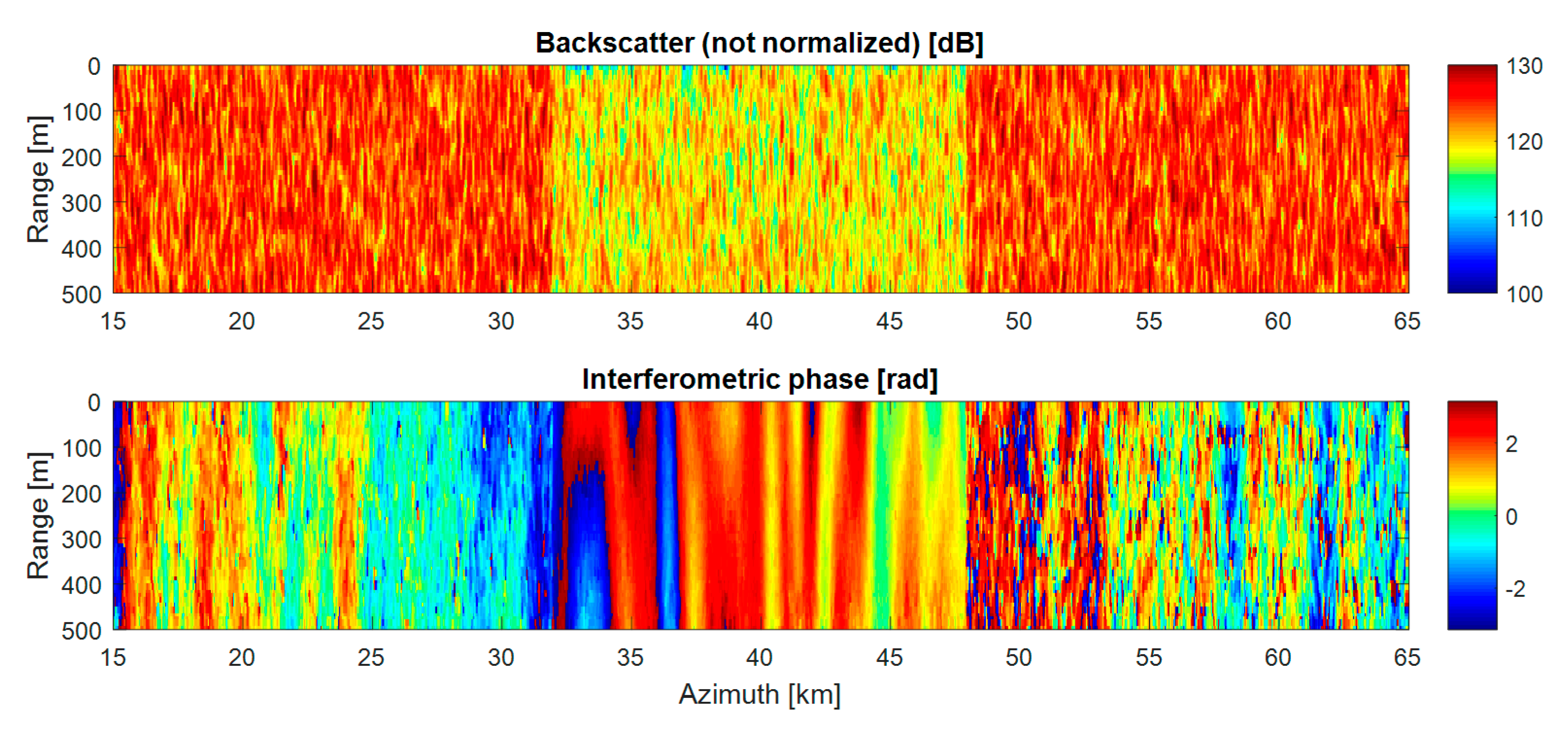
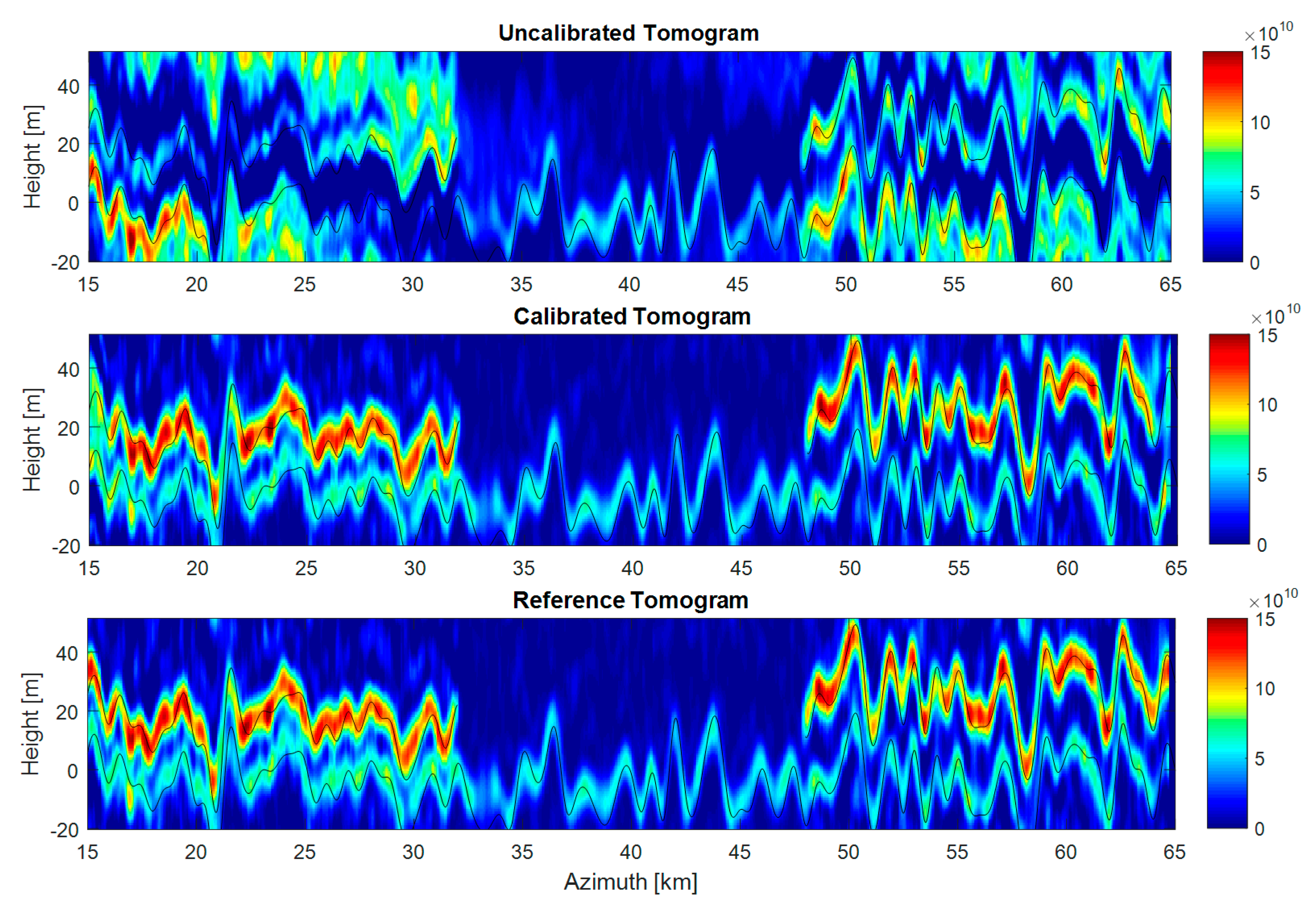
5. Simulation Results

Clock drift estimations were performed over a region of 500 m × 50 km (range × azimuth) using the two methods described in Section 3. For the MS inversion, 40 non-overlapping sub-bands dividing the azimuth bandwidth were processed, while for the MS difference, two non-overlapping sub-bands were processed. Both methods were able to accurately estimate the clock drift phase, with MS inversion yielding a lower Root-Mean-Square (RMS) error and more consistent results compared to MS difference (see Table 3). Simulation results are summarized in Figure 3, Figure 4 and Figure 5.

Table 3. RMS error of clock phase estimations (degrees) for the two methods, for each corrected image. Uncertainty values are due to the variations between simulation sets (see Section 4).

Image	MS Difference	MS Inversion
1	3.2 ± 0.6	0.9 ± 0.2
2	4.2 ± 1.1	1.1 ± 0.2
3	2.6 ± 0.9	0.8 ± 0.1
4	4.2 ± 1.8	1.2 ± 0.2
5	4.0 ± 1.6	1.2 ± 0.3

Figure 3. Estimation results for clock phase retrieval, shown for one set of simulations. Clock drift phases are shown on the left panel. Residuals of the estimations are shown on the right panel, for the two proposed methods.

Figure 4. Sample image simulated for a perpendicular baseline of 700 m. Upper: amplitude image (not normalized) in (dB). Lower: bistatic interferometric phase (rad), where it can be observed that the middle “bare soil” region has a less noisy phase than the surrounding regions, where volumetric decorrelation occurs.

Figure 5. Tomograms obtained from the simulated scenes. Upper: without phase calibration. Mid: computed from calibrated images with the MS inversion method. Lower: computed from reference images (generated without clock drift effect). Black lines represent the actual position of the scatterers. The peak power difference between tomographic profiles resulted in an RMS error of ΔP(z) = 0.02 ± 0.015 dB and negligible resolution loss.

6. Discussion

The presented phase compensation approach was capable of recovering the tomographic phases from the simulated bistatic images. The MS inversion method yielded a residual error of less than 2 degrees RMS, which was lower and with less dispersion than the MS difference method at the expense of increased computational complexity. A narrow range swath of 0.5 km was used to perform the estimations in our simulations, although processing larger swaths will improve its accuracy, since the final estimation is obtained as a range average.

One limitation of the current approach is that it is unable to recover the absolute clock offset, since the multisquint technique is not sensitive to errors that are constant in time.

It is also worth noting that that the phase due to the clock drift can only be partially separated from that caused by orbits uncertainties, as it can be observed from the topographic phase component:

$${\varphi }_{ORBIT}\left(x-r\psi ,r\right)=\frac{2\pi }{\lambda }\left(\left(\theta -{\theta }_0\right){ϵ}_{\perp }\left(x-\psi r\right)-{ϵ}_{\parallel }\left(x-\psi r\right)+\psi {ϵ}_{AT}\left(x-\psi r\right)\right).$$

(16)

Recalling Equations (6) and (7), it is clear that the parallel baseline error ${ϵ}_{\parallel }$ becomes mixed with the clock drift; these two are estimated and removed together. The phase term due to the perpendicular baseline error ${ϵ}_{\perp }$ can be separated with the aid of an external Digital Elevation Model because of its dependence with the look angle. The phase due to the along-track error ${ϵ}_{AT}$ can be neglected, since for orbital uncertainties in the order of 0.5 m of current systems, its impact on the estimation is less than 2 degrees across a 50-km scene.

7. Conclusions

We have analyzed the clock drift impact on non-cooperative bistatic SAR systems. It has been shown that, for current oscillators accuracies, the bistatic image focusing is not foreseen to be an issue. However, phase perturbations caused by slow-varying components of the drift can still be significant enough to require a compensation method. This is especially needed for highly demanding applications such as biomass estimation with tomography, where slight inaccuracies in the interferometric phases can significantly affect the quality of the derived tomograms.

Under the hypothesis that a coarse clock synchronization (time and frequency offsets) can be achieved with the methods described in Section 2, we proposed a calibration algorithm to estimate the clock phase perturbations from the multisquint interferometric phases. Its accuracy was tested on simulated images over volumetric targets, obtaining an accuracy better than 2 degrees RMS in the interferometric phase and a final accuracy of 0.02 ± 0.015 dB in the peak power of the derived tomograms. This allows us to conclude that the perturbations introduced by the clock drift in the bistatic interferometric phase can be accurately recovered and removed with the proposed method.

References

- Reigber, A.; Moreira, A. First demonstration of airborne SAR tomography using multibaseline L-band data. IEEE Trans. Geosci. Remote Sens. 2000, 38, 2142–2151. [Google Scholar] [CrossRef]
- Tebaldini, S. Single and multipolarimetric SAR tomography of forested areas: A parametric approach. IEEE Trans. Geosci. Remote Sens. 2010, 48, 2375–2387. [Google Scholar] [CrossRef]
- Ho Tong Minh, D.; Toan, T.L.; Rocca, F.; Tebaldini, S.; d’Alessandro, M.M.; Villard, L. Relating P-Band Synthetic Aperture Radar Tomography to Tropical Forest Biomass. IEEE Trans. Geosci. Remote Sens. 2014, 52, 967–979. [Google Scholar] [CrossRef]
- Moreira, A.; Krieger, G.; Hajnsek, I.; Papathanassiou, K.P.; Younis, M.; Lopez-Dekker, P.; Huber, S.; Villano, M.; Pardini, M.; Eineder, M.; et al. Tandem-L: A highly innovative bistatic SAR mission for global observation of dynamic processes on the Earth’s surface. IEEE Geosci. Remote Sens. Mag. 2015, 3, 8–23. [Google Scholar] [CrossRef]
- European Space Agency. SAOCOM Companion Mission Science Document; European Space Agency: Noordwijk, The Netherlands, 2014. [Google Scholar]
- Krieger, G.; Moreira, A. Multistatic SAR Satellite Formations: Potentials and Challenges. Proc. IGARSS 2005, 4, 2680–2684. [Google Scholar]
- Krieger, G.; Hajnsek, I.; Papathanassiou, K.P.; Younis, M.; Moreira, A. Interferometric Synthetic Aperture Radar (SAR) Missions Employing Formation Flying. Proc. IEEE 2010, 98, 816–843. [Google Scholar] [CrossRef]
- Breit, H.; Younis, M.; Balss, A.; Grigorov, C.; Hueso-Gonzalez, J.; Krieger, G. Bistatic Synchronisation and Processing of TanDEM-X Data. In Proceedings of the IEEE International Geoscience and Remote Sensing Symposium (IGARSS), Vancouver, BC, Canada, 24–29 July 2011; pp. 2424–2427. [Google Scholar]
- Weigt, M.; Grigorov, C.; Steinbrecher, U.; Schulze, D. TanDEM-X Mission: Long Term in Orbit Synchronisation Link Performance Analysis. In Proceedings of the IEEE 10th European Conference on Synthetic Aperture Radar, Berlin, Germany, 3–5 June 2014; pp. 1–4. [Google Scholar]
- Rodriguez-Cassola, M.; Prats-Iraola, P.; Nannini, M.; Lopez-Dekker, P.; Moreira, A.; Carnicero Dominguez, B. Calibration Concept for Weakly-Synchronised SAR Companion Missions: ESA’s SAOCOM/CS case. In Proceedings of the EUSAR 2016: 11th European Conference on Synthetic Aperture Radar, Hamburg, Germany, 6–9 June 2016; pp. 1–4. [Google Scholar]
- Rodriguez-Cassola, M.; Prats-Iraola, P.; Lopez-Dekker, P.; Reigber, A.; Krieger, G.; Moreira, A. Autonomous time and phase calibration of spaceborne bistatic SAR systems. In Proceedings of the EUSAR 2014: 10th European Conference on Synthetic Aperture Radar, Berlin, Germany, 3–5 June 2014. [Google Scholar]
- Rodriguez-Cassola, M.; Prats-Iraola, P.; Nannini, M.; López-Dekker, P.; Moreira, A.; Carnicero-Dominguez, B. Dedicated calibration concept for interferometric SAR companion missions. In Proceedings of the 2016 IEEE International Geoscience and Remote Sensing Symposium (IGARSS), Beijing, China, 10–15 July 2016; pp. 1416–1419. [Google Scholar]
- Krieger, G.; Younis, M. Impact of oscillator noise in bistatic and multistatic SAR. IEEE Geosci. Remote Sens. Lett. 2006, 3, 424–428. [Google Scholar] [CrossRef]
- Allan, D.W. The Statistics of Atomic Frequency Standards. Proc. IEEE 1966, 54, 221–230. [Google Scholar] [CrossRef]
- Candelier, V.; Canzian, P.; Lamboley, J.; Brunet, M.; Santarelli, G. Space qualified 5 MHz ultra stable oscillators. In Proceedings of the IEEE International Frequency Control Symposium and PDA Exhibition Jointly with the 17th European Frequency and Time Forum, Tampa, FL, USA, 4–8 May 2003; pp. 575–582. [Google Scholar]
- Gomba, G.; Parizzi, A.; De Zan, F.; Eineder, M.; Bamler, R. Toward Operational Compensation of Ionospheric Effects in SAR Interferograms: The Split-Spectrum Method. IEEE Trans. Geosci. Remote Sens. 2016, 54, 1446–1461. [Google Scholar] [CrossRef]
- Prats, P.; Mallorqui, J. Estimation of azimuth phase undulations with multisquint processing in airborne interferometric SAR images. IEEE Trans. Geosci. Remote Sens. 2003, 41, 1530–1533. [Google Scholar] [CrossRef]
- Mancon, S.; Monti Guarnieri, A.; Giudici, D.; Tebaldini, S. On the Phase Calibration by Multisquint Analysis in TOPSAR and Stripmap Interferometry. IEEE Trans. Geosci. Remote Sens. 2017, 55, 134–147. [Google Scholar] [CrossRef]
- Gomba, G.; De Zan, F.; Parizzi, A. Ionospheric Phase Screen and Ionospheric Azimuth Shift Estimation Combining the Split-Spectrum and Multi-Squint Methods. In Proceedings of the EUSAR 2016: 11th European Conference on Synthetic Aperture Radar, Hamburg, Germany, 6–9 June 2016; pp. 1–4. [Google Scholar]
- Gilbert, J.R.; Moler, C.; Schreiber, R. Sparse Matrices in MATLAB: Design and Implementation. SIAM J. Matrix Anal. Appl. 1992, 13, 333–356. [Google Scholar] [CrossRef]
- Li, D.; Rodriguez-Cassola, M.; Prats-Iraola, P.; López-Dekker, P.; Wu, M.; Detlefsen, J.; Moreira, A. Exact reverse backprojection for SAR raw data generation of natural scenes. In Proceedings of the 2016 IEEE International Geoscience and Remote Sensing Symposium (IGARSS), Beijing, China, 10–15 July 2016; pp. 3258–3261. [Google Scholar]
- Bauck, J.L.; Jenkins, W.K. Convolution-backprojection image reconstruction for bistatic synthetic aperture radar. In Proceedings of the IEEE International Symposium on Circuits and Systems, Portland, OR, USA, 8–11 May 1989; Volume 3, pp. 1512–1515. [Google Scholar]
- Frey, O.; Magnard, C.; Ruegg, M.; Meier, E. Focusing of Airborne Synthetic Aperture Radar Data from Highly Nonlinear Flight Tracks. IEEE Trans. Geosci. Remote Sens. 2009, 47, 1844–1858. [Google Scholar] [CrossRef]
- Papathanassiou, K.P.; Cloude, S.R. Single baseline polarimetric SAR interferometry. IEEE Trans. Geosci. Remote Sens. 2011, 39, 2352–2363. [Google Scholar] [CrossRef]
- Tebaldini, S.; Rocca, F. Multibaseline Polarimetric SAR Tomography of a Boreal Forest at P- and L-Bands. IEEE Trans. Geosci. Remote Sens. 2012, 50, 232–246. [Google Scholar] [CrossRef]
© 2017 by the authors. Licensee MDPI, Basel, Switzerland. This article is an open access article distributed under the terms and conditions of the Creative Commons Attribution (CC BY) license (http://creativecommons.org/licenses/by/4.0/).