
Reference Information Based Remote Sensing Image Reconstruction with Generalized Nonconvex Low-Rank Approximation

 ,
,  ,
,  ,
, 
Abstract
:
1. Introduction
2. Related Work
2.1. RSI Reconstruction with a Reference
2.2. Generalized RSI Reconstruction
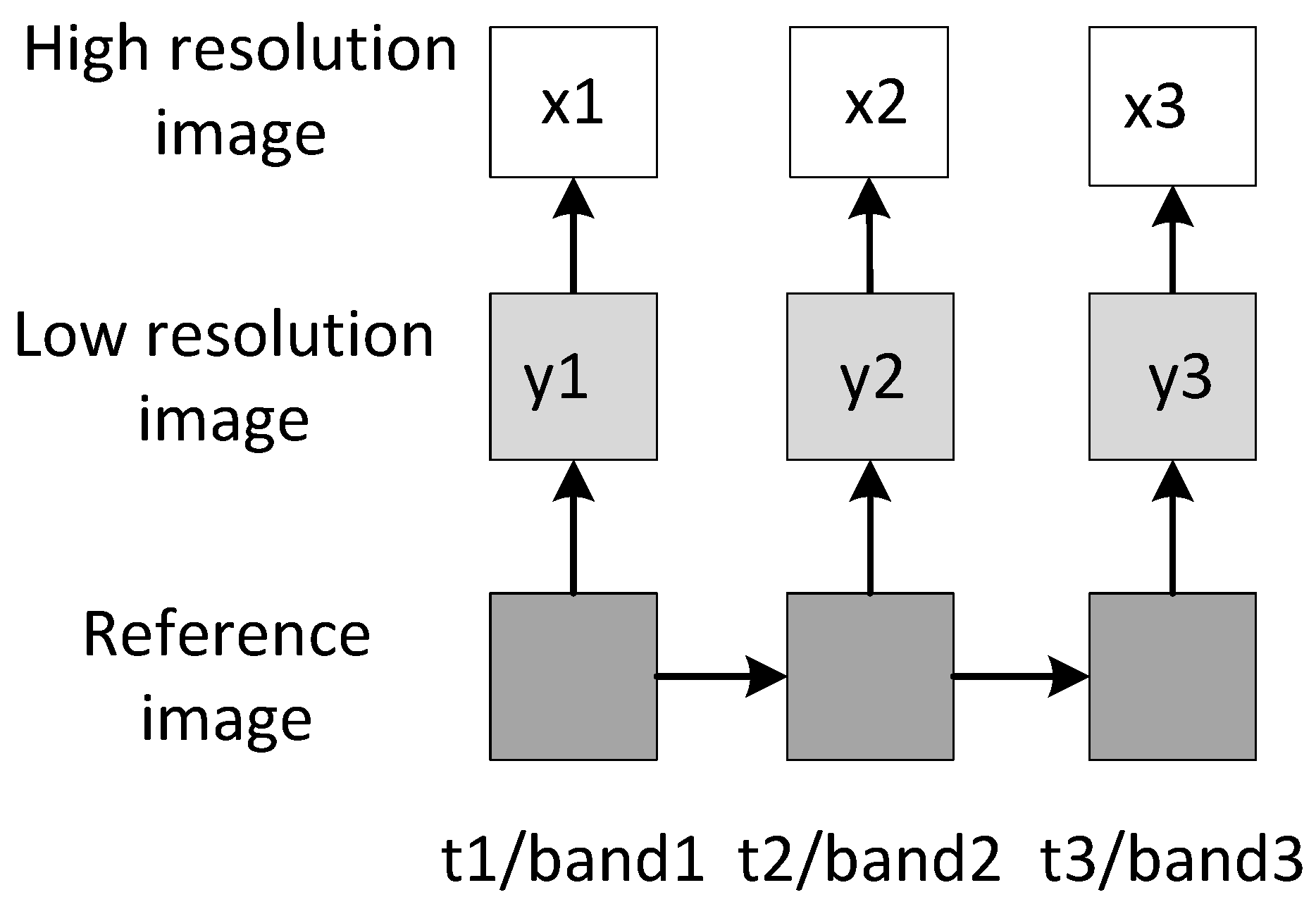
2.3. Reconstruction Model Based on Reference Images
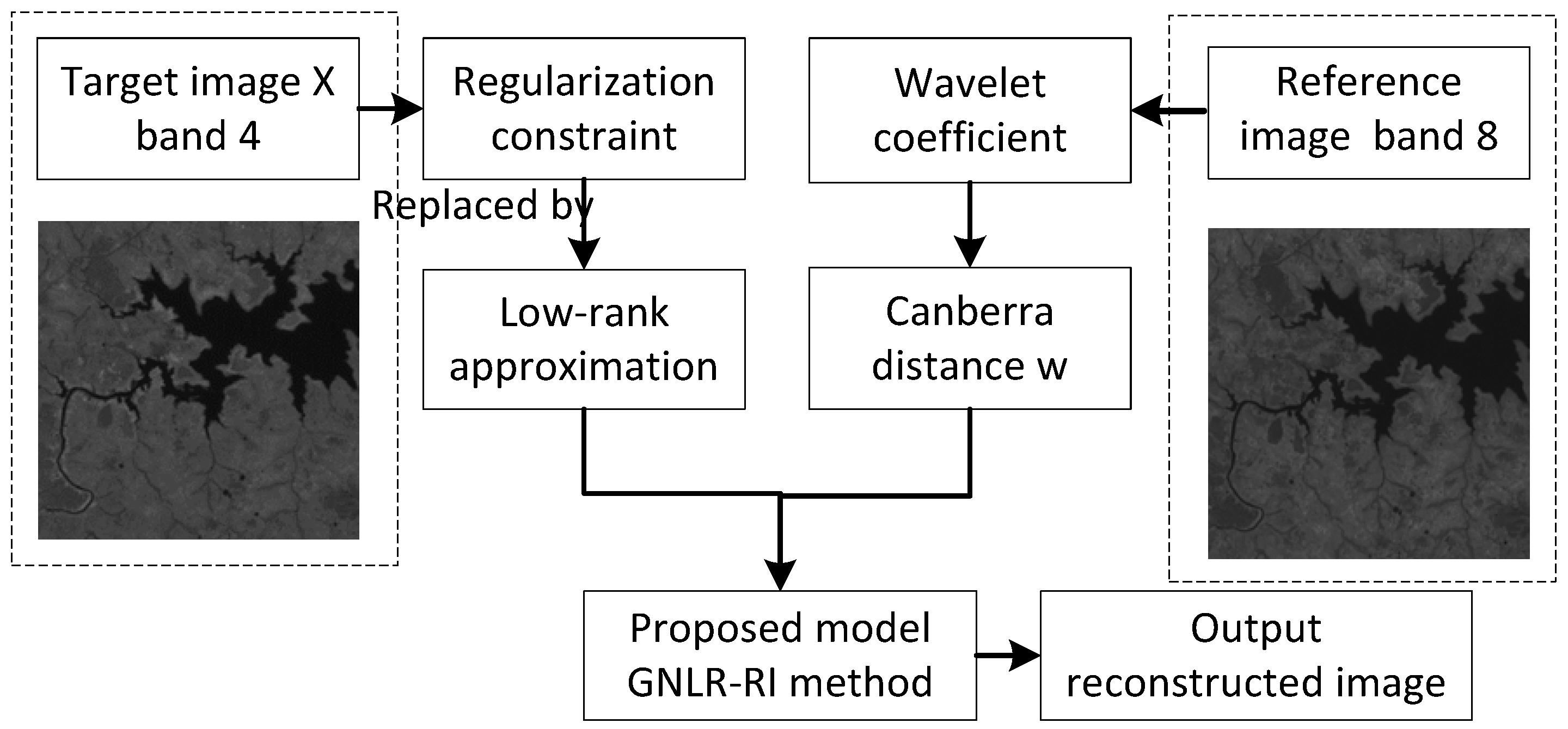
3. Generalized Nonconvex Low-Rank Approximation Model
4. Problem Definition
4.1. Solving the Proposed Model
| Algorithm 1: GNLR-RI. |
| Input: Sparse coefficient of reference image |
| Initialization: Set target wavelet coefficient α to zero; and α |
| While convergence criterion not met, do |
| 1. Compute the texture feature vectors F, of target wavelet coefficient α and reference wavelet coefficient using Equations (5) and (6). |
| 2. Add the constrained term to the compressed sensing target objective function. |
| 3. Add the low-rank approximation based on the reference image term. |
| 4. Solve the optimization problem Equation (20) via the conjunction gradient algorithm. |
| 5. Iteration: For , do |
| 1) Form a matrix making up similar patches of and set |
| 2) For , do |
| a) If , update the weights
|
| b) Compute via Equation (26) and output when . |
| End for |
| End for |
| 6. Solve the optimization problem Equation (28) via the conjunction gradient algorithm. |
| Output: |
5. Experiment Results
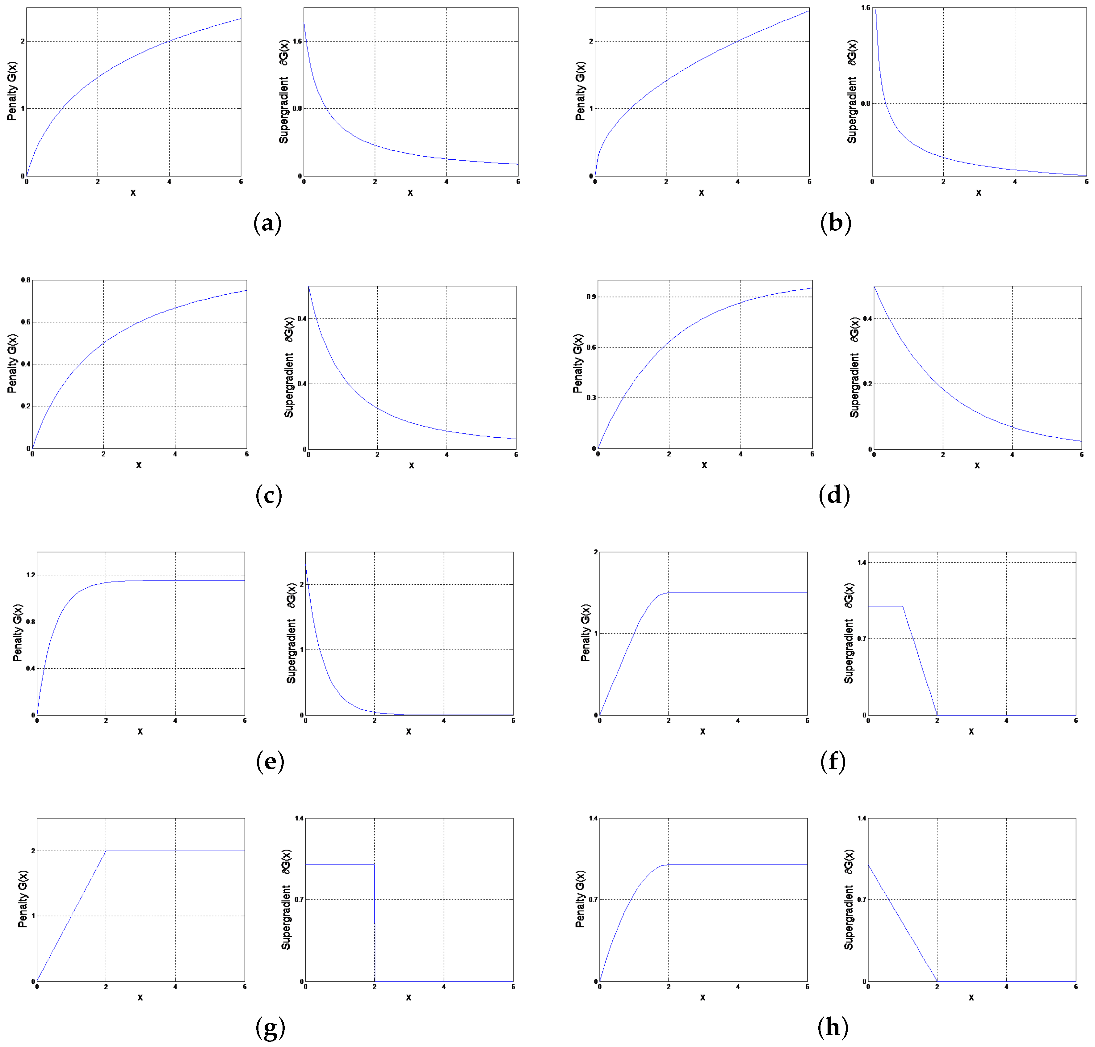
5.1. Evaluation of the Low Rank Penalty Function and Different Nonconvex Surrogate Functions
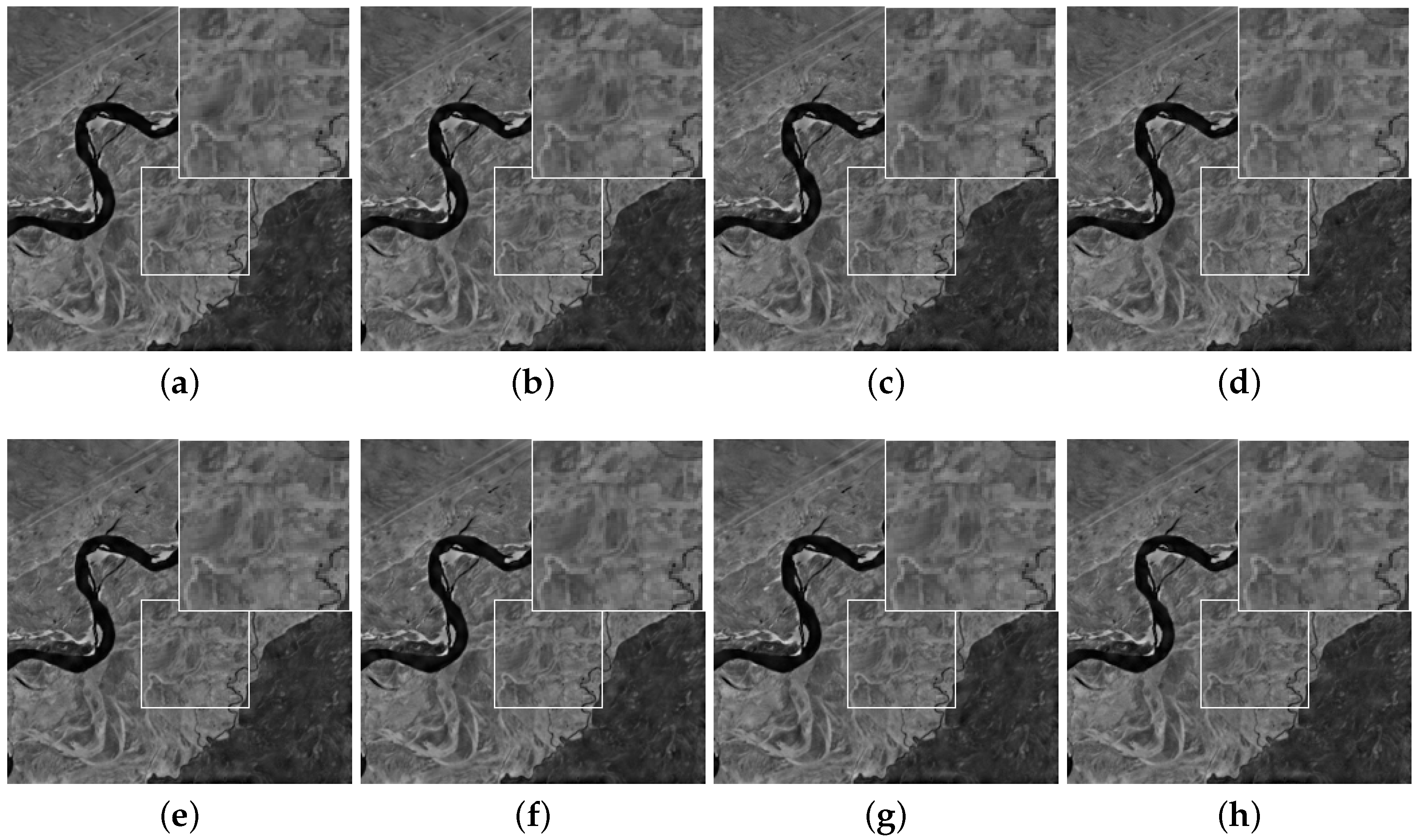
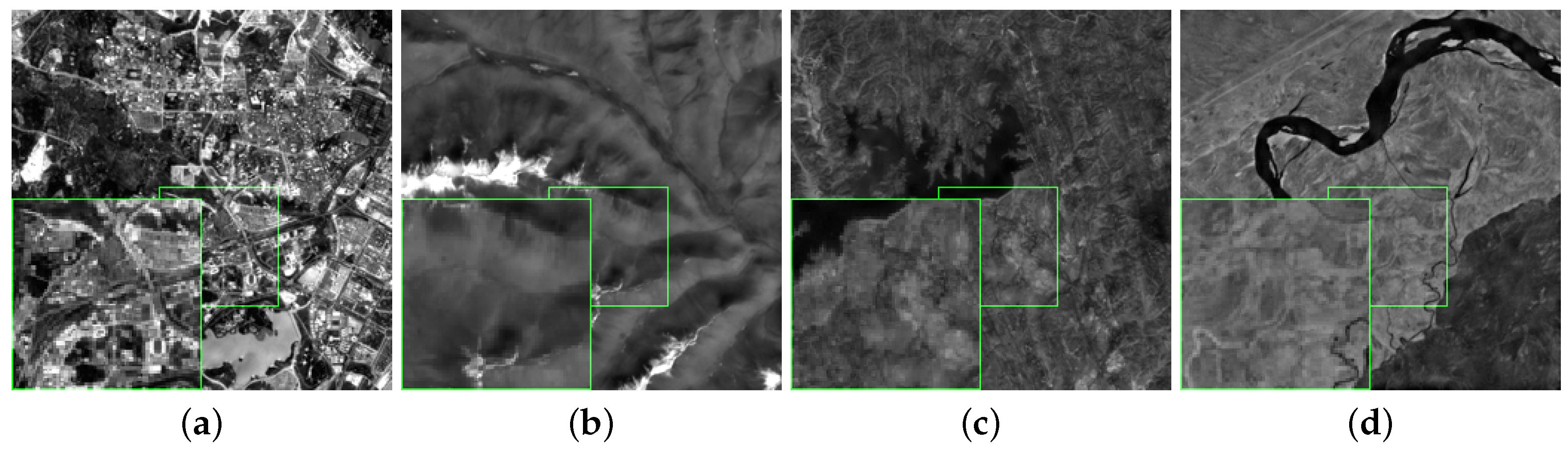
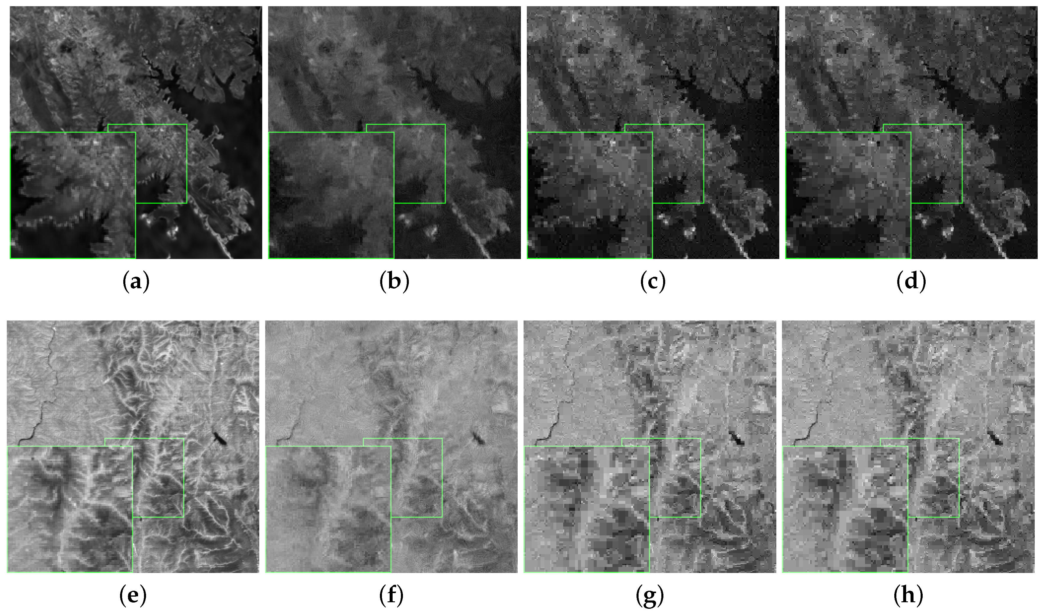
5.2. Performance Comparison for Single-Channel Compressed Sensing
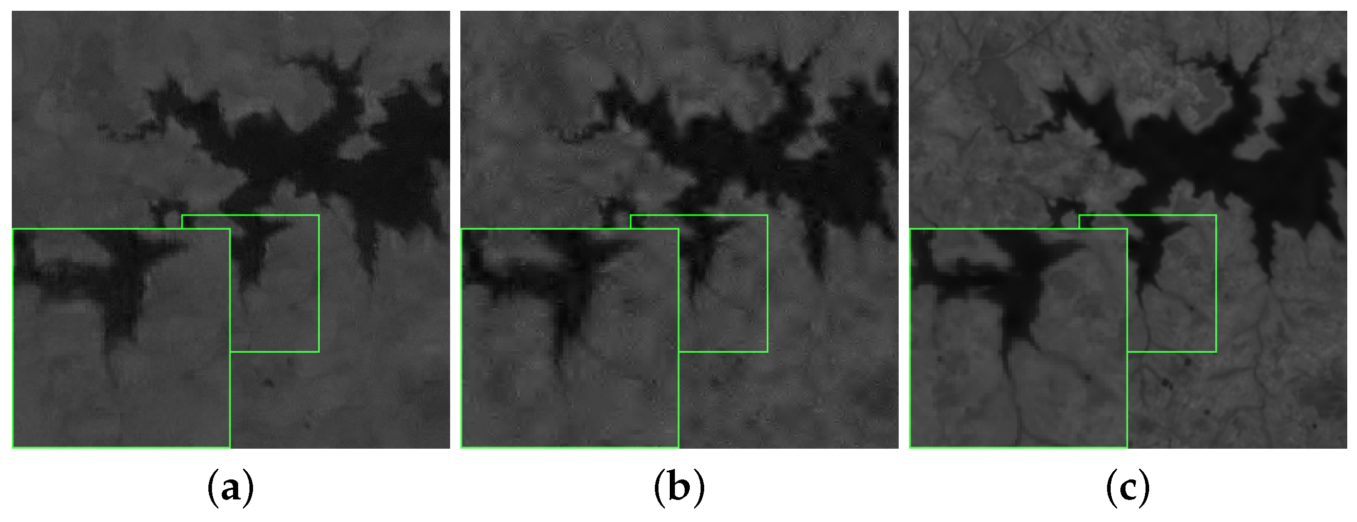
5.3. Multichannel Reconstruction with References
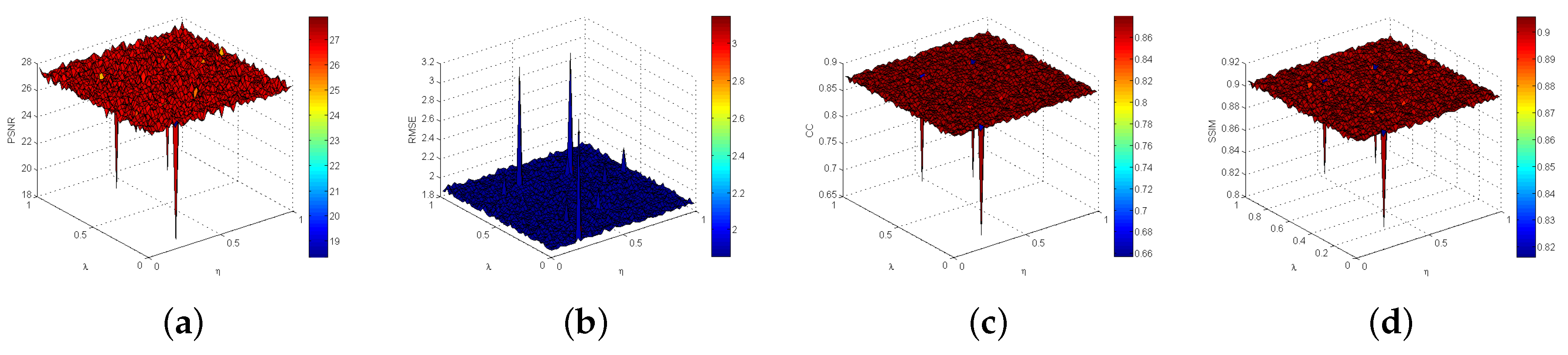
5.4. Parameter Evaluation
5.5. Performances with Varied Noise Levels
5.6. Computational Complexity
6. Conclusions
Acknowledgments
Author Contributions
Conflicts of Interest
References
- Li, X.; Shen, H.; Zhang, L.; Li, H. Sparse-based reconstruction of missing information in remote sensing images from spectral/temporal complementary information. ISPRS J. Photogramm. Remote Sens. 2015, 106, 1–15. [Google Scholar] [CrossRef]
- Wang, L.; Lu, K.; Liu, P. Compressed sensing of a remote sensing image based on the priors of the reference image. IEEE Geosci. Remote Sens. Lett. 2015, 12, 736–740. [Google Scholar] [CrossRef]
- Geng, H.; Liu, P.; Wang, L.; Chen, L. Compressed sensing based remote sensing image reconstruction using an auxiliary image as priors. In Proceedings of the 2014 IEEE International Geoscience and Remote Sensing Symposium (IGARSS), Quebec City, QC, Canada, 13–18 July 2014; pp. 2499–2502.
- Liu, P.; Huang, F.; Li, G.; Liu, Z. Remote-sensing image denoising using partial differential equations and auxiliary images as priors. IEEE Geosci. Remote Sens. Lett. 2012, 9, 358–362. [Google Scholar] [CrossRef]
- Hu, T.; Zhang, H.; Shen, H.; Zhang, L. Robust registration by rank minimization for fultiangle hyper/multispectral remotely sensed imagery. IEEE J. Sel. Top. Appl. Earth Observ. Remote Sens. 2014, 7, 2443–2457. [Google Scholar] [CrossRef]
- Dong, W.; Shi, G.; Li, X. Nonlocal image restoration with bilateral variance estimation: A low-rank approach. IEEE Trans. Image Process. 2013, 22, 700–711. [Google Scholar] [CrossRef] [PubMed]
- Dong, W.; Shi, G.; Li, X.; Ma, Y.; Huang, F. Compressive sensing via nonlocal low-rank regularization. IEEE Trans. Image Process. 2014, 23, 3618–3632. [Google Scholar] [CrossRef] [PubMed]
- Peng, L.; Eom, K.B. Restoration of multispectral images by total variation with auxiliary image. Opt. Lasers Eng. 2013, 51, 873–882. [Google Scholar]
- Peng, L.; Dingsheng, L.; Zhu, L. Total variation restoration of the defocus image based on spectral priors. Int. Soc. Opt. Photon. Remote Sens. 2010. [Google Scholar] [CrossRef]
- Madni, A.M. A systems perspective on compressed sensing and its use in reconstructing sparse networks. IEEE Syst. J. 2014, 8, 23–27. [Google Scholar] [CrossRef]
- Wei, L.; Prasad, S.; Fowler, J.E. Spatial information for hyperspectral image reconstruction from compressive random projections. IEEE Geosci. Remote Sens. Lett. 2013, 10, 1379–1383. [Google Scholar]
- Xiao, D.; Yunhua, Z. A novel compressive sensing algorithm for SAR imaging. IEEE J. Sel. Top. Appl. Earth Observ. Remote Sens. 2014, 7, 708–720. [Google Scholar]
- Fowler, J.E. Compressive-projection principal component analysis. IEEE Trans. Image Process. 2009, 18, 2230–2242. [Google Scholar] [CrossRef] [PubMed]
- Ly, N.H.; Du, Q.; Fowler, J.E. Reconstruction from random projections of hyperspectral imagery with spectral and spatial partitioning. IEEE J. Sel. Top. Appl. Earth Observ. Remote Sens. 2013, 6, 466–472. [Google Scholar] [CrossRef]
- Chen, C.; Wei, L.; Eric, W.T.; James, E.F. Reconstruction of hyperspectral imagery from random projections using multi-hypothesis prediction. IEEE Trans. Geosci. Remote Sens. 2014, 52, 365–374. [Google Scholar] [CrossRef]
- Qiegen, L.; Shanshan, W.; Ying, L. Adaptive dictionary learning in sparse gradient domain for image recovery. IEEE Trans. Image Process. 2013, 22, 4652–4663. [Google Scholar]
- Zhang, X.; Bai, T.; Meng, H.; Chen, J. Compressive sensing-based ISAR imaging via the combination of the sparsity and nonlocal total variation. IEEE Geosci. Remote Sens. Lett. 2014, 11, 990–994. [Google Scholar] [CrossRef]
- He, X.; Condat, L.; Chanussot, J.; Xia, J. Pansharpening using total variation regularization. In Proceedings of the 2012 IEEE International Geoscience and Remote Sensing Symposium (IGARSS), Munich, Germany, 22–27 July 2012; pp. 166–169.
- Zhang, H.; He, W.; Zhang, L.; Shen, H.; Yuan, Q. Hyperspectral image restoration using low-rank matrix recovery. IEEE Trans. Geosci. Remote Sens. 2014, 52, 4729–4743. [Google Scholar] [CrossRef]
- He, W.; Zhang, H.; Zhang, L.; Shen, H. Total variation regularized low-rank matrix factorization for hyperspectral image restoration. IEEE Trans. Geosci. Remote Sens. 2016, 54, 178–188. [Google Scholar] [CrossRef]
- Zhang, J.; Zhong, P.; Chen, Y.; Li, S. Regularized deconvolution network for the representation and restoration of optical remote sensing images. IEEE Trans. Geosci. Remote Sens. 2014, 52, 2617–2627. [Google Scholar] [CrossRef]
- Yue, L.; Shen, H.; Yuan, Q.; Zhang, L. A locally adaptive L1/L2 norm for multi-frame super-resolution of images with mixed noise and outliers. Signal Process. 2014, 105, 156–174. [Google Scholar] [CrossRef]
- Zheng, Z.; Xu, Y.; Yang, J.; Li, X.; Zhang, D. A survey of sparse representation: algorithms and applications. IEEE Access 2015, 3, 490–530. [Google Scholar] [CrossRef]
- Xiaobo, Q.; Di, G.; Bende, N.; Yingkun, H.; Yulan, L.; Cai, S.; Zhong, C. Undersampled MRI reconstruction with patch-based directional wavelets. Magn. Resonance Imaging 2012, 30, 964–977. [Google Scholar]
- Skretting, K.; Engan, K. Recursive least squares dictionary learning algorithm. IEEE Trans. Image Process 2010, 58, 2121–2130. [Google Scholar] [CrossRef]
- Aharon, M.; Elad, M.; Bruckstein, A. K-SVD: An algorithm for designing overcomplete dictionaries for sparse representation. IEEE Trans. Signal Process 2006, 54, 4311–4322. [Google Scholar] [CrossRef]
- Zobly, S.M.S.; Kadah, Y.M. Orthogonal matching pursuit and compressive sampling matching pursuit for Doppler ultrasound signal reconstruction. In Proceedings of the 2012 Cairo International, Biomedical Engineering Conference (CIBEC), Giza, Egypt, 20–22 December 2012; pp. 52–55.
- Ravazzi, C.; Fosson, S.M.; Magli, E. Distributed iterative thresholding for ℓ0/ℓ1-regularized linear inverse problems. IEEE Trans. Inf. Theory 2015, 61, 2081–2100. [Google Scholar] [CrossRef]
- Xiaoqun, Z.; Martin, B.; Xavier, B.; Stanley, O. Bregmanized nonlocal regularization for deconvolution and sparse reconstruction. SIAM J. Imaging Sci. 2010, 3, 253–276. [Google Scholar]
- Liu, Q.; Peng, X.; Liu, J.; Yang, D.; Liang, D. A weighted two-level bregman method with dictionary updating for nonconvex MR image reconstruction. J. Biomed. Imaging 2014. [Google Scholar] [CrossRef] [PubMed]
- Yang, S.; Liu, Z.; Wang, M.; Sun, F.; Jiao, L. Multitask learning and sparse representation based super-resolution reconstruction of synthetic aperture radar images. In Proceedings of the 2011 International Workshop on Multi-Platform/Multi-Sensor Remote Sensing and Mapping (M2RSM), Xiamen, China, 10–12 January 2011; pp. 1–5.
- Fazel, M.; Hindi, H.; Boyd, S.P. Log-det heuristic for matrix rank minimization with applications to Hankel and Euclidean distance matrices. Proc. Am. Control Conf. 2003, 3, 2156–2162. [Google Scholar]
- Gasso, G.; Rakotomamonjy, A.; Canu, S. Recovering sparse signals with a certain family of nonconvex penalties and DC programming. IEEE Trans. Signal Process. 2009, 57, 4686–4698. [Google Scholar] [CrossRef]
- Chartrand, R. Exact reconstruction of sparse signals via nonconvex minimization. IEEE Signal Process. Lett. 2007, 14, 707–710. [Google Scholar] [CrossRef]
- Trzasko, J.; Manduca, A. Highly undersampled magnetic resonance image reconstruction via homotopic-minimization. IEEE Trans. Med. Imaging 2009, 28, 106–121. [Google Scholar] [CrossRef] [PubMed]
- Canyi, L.; Jinhui, T.; Shuicheng, Y.; Zhouchen, L. Generalized nonconvex nonsmooth low-rank minimization. In Proceedings of the IEEE Conference onComputer Vision and Pattern Recognition (CVPR), Zurich, Switzerland, 6–12 September 2014; pp. 4130–4137.
- Friedman, J.H. Fast sparse regression and classification. Int. J. Forecast. 2012, 28, 722–738. [Google Scholar] [CrossRef]
- Frank, L.E.; Friedman, J.H. A statistical view of some chemometrics regression tools. Technometrics 1993, 35, 109–135. [Google Scholar] [CrossRef]
- Geman, D.; Yang, C. Nonlinear image recovery with half-quadratic regularization. IEEE Trans. Image Process. 1995, 4, 932–946. [Google Scholar] [CrossRef] [PubMed]
- Gao, C.; Wang, N.; Yu, Q.; Zhang, Z. A Feasible Nonconvex Relaxation Approach to Feature Selection. Available online: http://bcmi.sjtu.edu.cn/ zhzhang/papers/etp.pdf (accessed on 4 March 2016).
- Fan, J.; Li, R. Variable selection via nonconcave penalized likelihood and its oracle properties. J. Am. Stat. Assoc. 2001, 96, 1348–1360. [Google Scholar] [CrossRef]
- Tong, Z. Analysis of multi-stage convex relaxation for sparse regularization. J. Mach. Learn. Res. 2010, 11, 1081–1107. [Google Scholar]
- CunHui, Z. Nearly unbiased variable selection under minimax concave penalty. Ann. Stat. 2010, 894–942. [Google Scholar]
- Chen, C.; Eric, W.T.; James, E.F. Compressed-sensing recovery of images and video using multi-hypothesis predictions. In Proceedings of the 45th Asilomar Conference on Signals, Systems, and Computers, Pacific Grove, CA, USA, 6–9 November 2011; pp. 1193–1198.
- Zhang, J.; Zhao, D.; Zhao, C.; Xiong, R.; Ma, S.; Gao, W. Image compressive sensing recovery via collaborative sparsity. IEEE J. Emerg. Sel. Top. Circuits Syst. 2012, 2, 380–391. [Google Scholar] [CrossRef]
- Zhanga, J.; Zhaob, C.; Zhaoa, D.; Gaob, W. Image compressive sensing recovery using adaptively learned sparsifying basis via L0 minimization. Signal Process. 2014, 103, 114–126. [Google Scholar] [CrossRef]

| Nonconvex Surrogate Functions | Formulation | Super-Gradient |
|---|---|---|
| Log | ||
| Lp | ||
| Geman | ||
| Lap | ||
| Etp | ||
| Scad | ||
| Cappedl1 | ||
| Mcp |
| Functions | Landsat 8 | MODIS | Landsat 7 |
|---|---|---|---|
| Log | 32.655/3.263 | 27.843/3.274 | 25.616/11.477 |
| Lp | 32.804/5.463 | 26.068/3.266 | 25.569/11.259 |
| Geman | 32.655/5.434 | 26.194/3.253 | 25.964/10.922 |
| Lap | 32.714/5.387 | 27.193/3.312 | 25.580/10.843 |
| Etp | 32.803/5.466 | 27.310/3.282 | 25.681/11.499 |
| Scad | 32.667/5.435 | 26.223/3.293 | 25.958/11.319 |
| Cappedl1 | 32.695/5.478 | 27.081/3.305 | 25.757/11.271 |
| Mcp | 32.752/5.499 | 26.251/3.268 | 25.863/11.018 |
| Images | Patch Sizes | PSNR | RMSE | CC | SSIM |
|---|---|---|---|---|---|
| (1) | 2 × 2 | 24.006 | 17.930 | 0.958 | 0.898 |
| (1) | 4 × 4 | 24.128 | 17.780 | 0.958 | 0.897 |
| (1) | 6 × 6 | 24.212 | 17.777 | 0.958 | 0.896 |
| (1) | 8 × 8 | 24.287 | 17.937 | 0.957 | 0.896 |
| (2) | 2 × 2 | 30.469 | 8.908 | 0.980 | 0.844 |
| (2) | 4 × 4 | 30.615 | 8.709 | 0.980 | 0.832 |
| (2) | 6 × 6 | 30.552 | 8.816 | 0.979 | 0.828 |
| (2) | 8 × 8 | 30.806 | 8.823 | 0.979 | 0.832 |
| (3) | 2 × 2 | 24.404 | 11.264 | 0.925 | 0.802 |
| (3) | 4 × 4 | 24.485 | 11.470 | 0.921 | 0.782 |
| (3) | 6 × 6 | 24.936 | 11.295 | 0.922 | 0.790 |
| (3) | 8 × 8 | 23.919 | 11.822 | 0.914 | 0.773 |
| (4) | 2 × 2 | 24.128 | 17.780 | 0.958 | 0.897 |
| (4) | 4 × 4 | 24.212 | 17.777 | 0.958 | 0.896 |
| (4) | 6 × 6 | 24.287 | 17.937 | 0.957 | 0.896 |
| (4) | 8 × 8 | 30.469 | 8.908 | 0.980 | 0.844 |
| Landsat 8 Bands 4/5/6 | Google Earth Bands 1/2/3 | |||||||||
|---|---|---|---|---|---|---|---|---|---|---|
| PSNR | SAM | RASM | ERGAS | Q4 | PSNR | SAM | RASM | ERGAS | Q4 | |
| OMP | 17.644 | 0.092 | 0.162 | 0.041 | 0.986 | 19.741 | 0.018 | 0.059 | 0.015 | 0.944 |
| CoSaMP | 17.327 | 0.074 | 0.146 | 0.037 | 0.989 | 19.462 | 0.017 | 0.054 | 0.014 | 0.954 |
| NLR-CS-baseline | 17.294 | 0.195 | 0.434 | 0.109 | 0.865 | 30.055 | 0.010 | 0.062 | 0.016 | 0.930 |
| MH-BCS-SPL | 27.568 | 0.162 | 0.165 | 0.041 | 0.985 | 31.963 | 0.010 | 0.071 | 0.018 | 0.917 |
| RCoS | 18.412 | 0.140 | 0.511 | 0.128 | 0.820 | 23.495 | 0.025 | 0.219 | 0.054 | 0.607 |
| ALSB | 28.753 | 0.138 | 0.144 | 0.036 | 0.989 | 32.821 | 0.028 | 0.064 | 0.016 | 0.932 |
| reference | band 8 | gray | ||||||||
| GNLR-RI-Log | 22.459 | 0.023 | 0.223 | 0.762 | 0.951 | 41.967 | 0.009 | 0.018 | 0.005 | 0.995 |
| λ | η | Landsat 8 | MODIS | ||
|---|---|---|---|---|---|
| Band 4 | Band 8 | Band 2 | Band 3 | ||
| 0.25 | 0.07 | 24.668 | 26.674 | 24.229 | 27.311 |
| 0.45 | 0.45 | 25.834 | 27.050 | 23.763 | 26.969 |
| 0.67 | 0.33 | 24.843 | 26.702 | 23.798 | 27.427 |
| 0.87 | 0.25 | 24.474 | 26.902 | 24.027 | 27.604 |
| GNLR-RI-Log | NLR-CS-baseline | CoSaMP | OMP | GNLR-RI-Log | NLR-CS-baseline | CoSaMP | OMP | |
|---|---|---|---|---|---|---|---|---|
| 32.863 | 23.502 | 28.754 | 28.021 | 31.225 | 22.025 | 24.803 | 24.274 | |
| 32.786 | 23.499 | 28.202 | 27.664 | 31.279 | 22.023 | 24.610 | 24.122 | |
| 32.615 | 23.496 | 26.798 | 26.879 | 30.994 | 22.022 | 23.974 | 23.717 | |
| 32.639 | 23.483 | 25.103 | 25.651 | 30.874 | 22.015 | 23.0007 | 23.086 |
| Methods | OMP | CoSaMP | NLR-CS-baseline | MH-BCS-SPL | RCoS | ALSB | GNLR-RI-Log |
|---|---|---|---|---|---|---|---|
| Runtime (s) | 0.106/iter. | 0.031/iter. | 3.56/iter. | 1.39/iter. | 21.08/iter. | 17.11/iter. | 0.22/iter. |
© 2016 by the authors; licensee MDPI, Basel, Switzerland. This article is an open access article distributed under the terms and conditions of the Creative Commons Attribution (CC-BY) license (http://creativecommons.org/licenses/by/4.0/).
Share and Cite
Lu, H.; Wei, J.; Wang, L.; Liu, P.; Liu, Q.; Wang, Y.; Deng, X. Reference Information Based Remote Sensing Image Reconstruction with Generalized Nonconvex Low-Rank Approximation. Remote Sens. 2016, 8, 499. https://doi.org/10.3390/rs8060499
Lu H, Wei J, Wang L, Liu P, Liu Q, Wang Y, Deng X. Reference Information Based Remote Sensing Image Reconstruction with Generalized Nonconvex Low-Rank Approximation. Remote Sensing. 2016; 8(6):499. https://doi.org/10.3390/rs8060499
Chicago/Turabian StyleLu, Hongyang, Jingbo Wei, Lizhe Wang, Peng Liu, Qiegen Liu, Yuhao Wang, and Xiaohua Deng. 2016. "Reference Information Based Remote Sensing Image Reconstruction with Generalized Nonconvex Low-Rank Approximation" Remote Sensing 8, no. 6: 499. https://doi.org/10.3390/rs8060499
APA StyleLu, H., Wei, J., Wang, L., Liu, P., Liu, Q., Wang, Y., & Deng, X. (2016). Reference Information Based Remote Sensing Image Reconstruction with Generalized Nonconvex Low-Rank Approximation. Remote Sensing, 8(6), 499. https://doi.org/10.3390/rs8060499