Abstract
Time-series SAR/InSAR techniques have proven to be effective tools for measuring landslide movements over large regions. Prior studies of these techniques, however, have focused primarily on technical innovation and applications, leaving coupling analysis of slope displacements and trigging factors as an unexplored area of research. Linking potential landslide inducing factors such as hydrology to SAR/InSAR derived displacements is of crucial importance for understanding landslide deformation mechanisms and could support the development of early-warning systems for disaster mitigation and management. In this study, a sequential data assimilation method named the Ensemble Kalman filter (EnKF), is adopted to explore the response mechanisms of the Shuping landslide movement in relation to hydrological factors. Previous research on the Shuping landslide area shows that the reservoir water level and rainfall are the two main triggering factors in slope failures. To extract the time-series deformations for the Shuping landslide area, Pixel Offset Tracking (POT) technique with corner reflectors was adopted to process the TerraSAR-X StripMap (SM) and High-resolution Spotlight (HS) images. Considering that these triggering factors are the primary causes of displacement fluctuations in periodic displacement, time-series decomposition was carried out to extract the periodic displacement from the POT measurements. The correlations between the periodic displacement and the inducing factors were qualitatively estimated through a grey relational analysis. Based on this analysis, the EnKF method was adopted to explore the response relationships between the displacements and triggering factors. Preliminary results demonstrate the effectiveness of EnKF in studying deformation response mechanisms and understanding landslide development processes.
1. Introduction
Landslides are a serious problem that can cause great loss to life and property. In the last century, due to global climate change and human impact on the environment, landslides have occurred with increasing frequency with corresponding economic losses and fatalities [1,2,3]. The Qianjiangping landslide located near Shuping for example, moved rapidly on 14 July 2003 and killed 24 people with the direct economic losses of about seven million USD [4]. Deformation monitoring is therefore essential since it can help us understand the characteristics and trends in landslide evolution and is particularly important for the development of preventative measures such as disaster forecasting and early warning systems [5,6,7].
In recent years, time-series SAR/InSAR techniques have been successfully used for detecting earth surface deformation, including applications for landslide monitoring. These techniques include Persistent Scatterer SAR Interferometry (PSInSARTM) [8], Small Baselines (SBAS) [9], Stable Point Network (SPN) [10], Interferometric Point Target Analysis (IPTA) [11], Coherent Pixels Technique (CPT) [12], Advanced InSAR algorithm (SqueeSAR) [13], Pixel Offset Tracking (POT) [14] and other InSAR Time Series Analysis (TSA) techniques [15]. All these techniques permit observation of the deformation distribution over the aerial extent of a landslide, unlike ground measurement techniques such as GPS measurements that monitor a limited set of points [16]. To date, studies have focused primarily on technical innovation and applications, but few have considered the interpretation of landslide displacement measurements derived from SAR/InSAR images in relation to potential triggering factors, although this work is of crucial importance to understand deformation mechanisms and assist early-warning and disaster forecasting.
To extend this research, we propose a data assimilation methodology that enables a coupled analysis between time-series SAR measurements and hydrological data. Data assimilation makes use of all available information from measurements and models to estimate unknowns, thereby reducing predictive uncertainties [17,18,19]. This method has been examined and applied in a number of fields such as atmospheric and oceanic modelling for numerical prediction [19], regional- to global-scale hydrometeorology for reflecting the land surface-atmosphere interaction [20], and catchment scale hydrology for parameter estimation and hydrological analysis [21]. However, there are few applications of data assimilation in landslide disaster research. We investigated the feasibility of this methodology to study the deformation mechanism of the Shuping landslide area in relation to hydrological data, e.g., water level and rainfall.
The Shuping landslide area is near the Three Gorges Reservoir. Previous studies revealed that the Shuping slope stability was affected by the fluctuation of water level and rainfall, exhibiting a maximum accumulative deformation of more than 1 m during 2008 and 2010 [22]. In a previous study, we investigated the effectiveness of a modified POT method for fast-moving landslide monitoring at the Shuping landslide site [22]. The deformation results were consistent with historic displacement measurements acquired by GPS [23]. Coupling analysis, however, between the slope displacements as derived from the POT technique and potential landslide inducing factors such as hydrology at Shuping region is still an unexplored area of research.
In this paper, we present a new approach that applies EnKF to fill the gap in the research that relates SAR/InSAR derived displacements to deformation mechanisms. The geological and topographical conditions accounting for relatively stable long-term trends are not considered in this paper, only the seasonally changing triggering factors related to periodic displacement fluctuation [24,25,26]. Corner reflectors installed at/near the landslide zone served as point targets to measure slope movements using the modified POT technique. A time-series decomposition method was used to separate the POT displacement into periodic and long-term trend terms prior to analysis of the interactions between landslide movements and hydrological factors. We conducted a grey relational analysis and thus qualitatively evaluated the role of hydrological factors in the variation of periodic displacement. In order to understand how inducing factors affect the development processes of Shuping landslides, a sequential data assimilation method, the Ensemble Kalman filter (EnKF) was adopted as it incorporates the available observations sequentially in time to explore the relationship between the landslide periodic motion and hydrological factors. Predictions based on StripMap (SM) mode and High-resolution Spotlight (HS) mode TerraSAR-X imagery were compared and analyzed in relation to fluctuation changes in the water level and rainfall. Preliminary results demonstrate the feasibility of our proposed method for understanding the response relationship between POT derived landslide movements and hydrological factors.
2. Methodology
2.1. Measuring Landslide Deformation with SAR/InSAR Data
Advanced remote sensing techniques based on Synthetic Aperture Radar (SAR) data are powerful methods for detecting and monitoring gradual ground surface deformations at a reasonable cost. Several authors have applied Interferometric Synthetic Aperture Radar (InSAR) to update landslide inventories and the activity status of slope deformations at a regional scale [27,28,29,30,31,32], but some drawbacks exist with regards to temporal and spatial decorrelations and the atmospheric phase screen effects [30,33].
These limitations have been partially resolved by time-series InSAR techniques, such as persistent scatterer SAR interferometry (PSInSAR™) [8], small baselines (SBAS) [9] or SqueeSAR [13,34]. These techniques make use of large sets of SAR images acquired at different times over the same area, permitting observation of the temporal evolution of surface deformations. However, these advanced time-series InSAR method cannot effectively extract surface displacement in areas with dense vegetation coverage and mutation surface deformation due to loss of coherence [35,36,37].
The POT technology is based on amplitude cross-correlation between SAR images, and can make up for the limitations of InSAR technology [14]. If stable Point Targets (PT), such as corner reflectors, are used, displacement can be measured at a cm-level accuracy [22]. POT technology has been recognized as an effective and robust tool for capturing the fast movement of the land surface caused by events such as earthquakes, landslides, and glacier motions [22,38,39,40].
In our previous study, a modified POT technique was employed to detect the deformation at the Shuping landslide area [22]. Two stacks of TerraSAR-X datasets acquired from 2008 to 2010 were analyzed to characterize the historic evolution of the Shuping landslide. In this study, corner reflectors installed at/near the landslide zone were utilized as PTs to analyze the spatial-temporal pattern of landslide deformations. Consequently, displacement measurements at these PTs were reasonably considered as a surrogate for local landslide deformations and adopted in a response analysis. The process flow of our proposed POT is illustrated in Figure 1—the details of this technique can be found in [22].
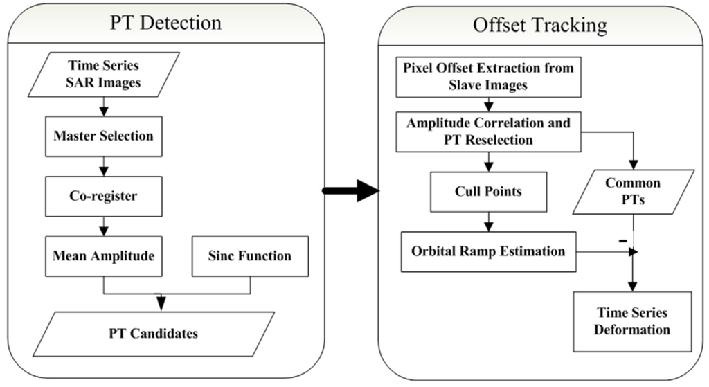
Figure 1.
The process flow of PT offset tracking.
2.2. Methods for Time-Series Decomposition
In this study, we conducted a coupling analysis between the POT time-series measurements and the landslide destabilizing factors, e.g., the fluctuation of the reservoir water level and rainfall. Assuming that these hydrological factors with seasonal variations are the primary cause of displacement fluctuations [24,25,26], time-series decomposition is needed to separate displacement extracted by the POT technique into a trend term and a periodic term. The time-series decomposition requires input data with the same time intervals. Because the time-series POT measurements are incomplete, as some dates are missing, a cubic spline interpolation was thus adopted to generate data for these missing but expected revisit times.
The processed displacement in the study area is a nonlinear, nonstationary curve influenced by reservoir level fluctuations, seasonal precipitation and other random disturbances. To eliminate the effect caused by random noise, de-noising processing must be applied to measurements. Then, the displacement can be separated into trend and periodic components. The trend component was computed by a quadratic polynomial fitting method and the seasonal component was calculated using the difference between the displacement time-series and the previously estimated trend component. The processing procedure for time series decomposition is shown in Figure 2.
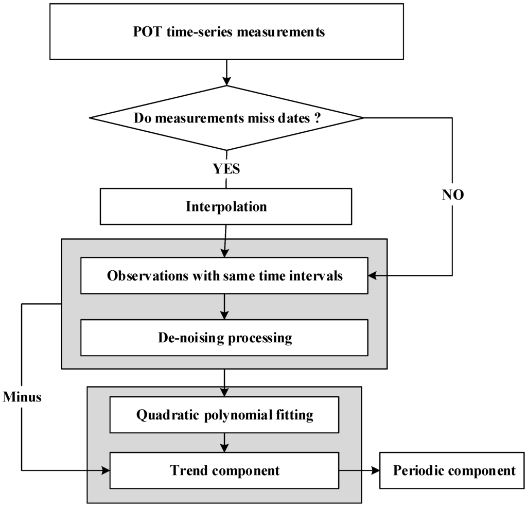
Figure 2.
The flow chart for time series decomposition.
The moving average method is believed to be an effective way to reduce the short-term uncertainty caused by random disturbances and highlights longer-term cycles or trends [41,42]; thus, it was applied to the displacement time-series derived from the SM stack. The time intervals for the moving average method, were set at less than the cycle of the periodical factors to protect the seasonal signal from damage. In this study, 16 historical series of displacements before 15 February 2009 in the SM stack were set as the first moving window to conduct the moving average analysis, roughly one half-cycle of the hydrological factors (approximately one cycle occurs per year). However, the HS stack derived deformation time-series has only one complete cycle (one cycle per year) during the period from February 2009 to April 2010. Therefore, it was impossible to use 16 historical series observations to conduct the moving average analysis and at the same time obtain a complete period for the cyclical variation of displacement. An alternative de-noising method must be found.
In the grey forecasting model, the Accumulated Generating Operation (AGO) is adopted in time-series data processing since it can weaken the randomness of the raw data and remove the interference from noise [43,44]. In this study, the capacity of AGO to eliminate random noise in deformations derived from SAR images will be explored. The time series of displacements at the corner reflectors derived from SM dataset were employed to noise reduction using both the moving average method and the AGO method. To estimate the feasibility of the AGO method, the resulting seasonal deformations from the AGO method will be compared with that from the moving average method. These results are shown and discussed in Section 4.2.
2.3. Coupling Analysis Scheme Based on Data Assimilation
EnKF is a sequential data assimilation method that can incorporate available observations sequentially in time. It was first introduced by Envenson [45], and later clarified by Burgers et al. [46] and Van Leewen [47]. The EnKF based upon the Monte Carlo method, applies an ensemble of model states to represent model estimation and continuously updates error statistics over time [20]. An analysis scheme operates directly on the ensemble of model states when observations become available for data assimilation. The EnKF has been applied in a number of fields such as atmospheric and oceanic modelling for numerical prediction [18], regional- to global-scale hydrometeorology for reflecting the land surface-atmosphere interaction [20], and catchment scale hydrology for parameter estimation and hydrological analysis [21]. However, EnKF or indeed other data assimilation methods have rarely been applied in landslide research. Given its widespread use in many domains, we adopted the EnKF data assimilation method to study the deformation mechanism of a landslide in a reservoir with the influence of hydrological factors, water level and rainfall.
2.3.1. Dynamic Process of a Landslide Evolution
Landslide evolution can be considered as a differential function that temporally integrates dynamic states and model parameters under a driving force, such as rainfall or the reservoir level. The functions for a landslide process can be denoted as a nonlinear stochastic process,
where t denotes the time step, S is the state vector consisting of model parameters and variables, f is the nonlinear forecast operator, U is a set of externally time-dependent forcing variables (e.g., rainfall), and the noise term ω accounts for model error.
Observations using different instruments or techniques can be directly or indirectly related to the model states and denoted as,
where y denotes the observation vector, H is the observation operator that represents the deterministic relationship between observation y and the true state S. Before data assimilation, the POT technique is adopted to retrieve landslide displacement from original SAR signals/images; then, time-series decomposition is applied to get the periodic component from the POT measurements. Because the state vectors include periodic displacement, we designated a linear observation operator with only 0 s and 1 s as its entries. The observations are perturbed by white noise ε that represents the possible measurement errors. This noise is mutually uncorrelated in space and time, with means equaling zero and standard deviations scaling to the current values of variables and dependent on the measurement accuracy of the monitoring tools and methods. For example, the achievable accuracy of displacement measured by POT can be theoretically expressed as [48]:
where γ is the coherence value and N is the number of pixels within the estimation window, equal to 11 × 11 in our study. The coherence of the corner reflectors usually ranges from 0.8 to 0.9. Selecting 0.8 as the coherence value in our study yielded a calculated accuracy of approximately 0.0364 m. Consequently, we applied a scaler factor of 0.4 to the values for periodic term displacement based on the POT results.
In order to get optimal estimates for the parameters and states of interest, we combined complementary information from Equations (1) and (2), which is the basic idea of data assimilation. The EnKF sequential data assimilation method uses an ensemble of state vectors (a priori St) to represent the true probability distribution of the state vectors (a posteriori St+1) by integrating the priori forward in time as observations (yt) become available. The sequential data assimilation process is illustrated in Figure 3.
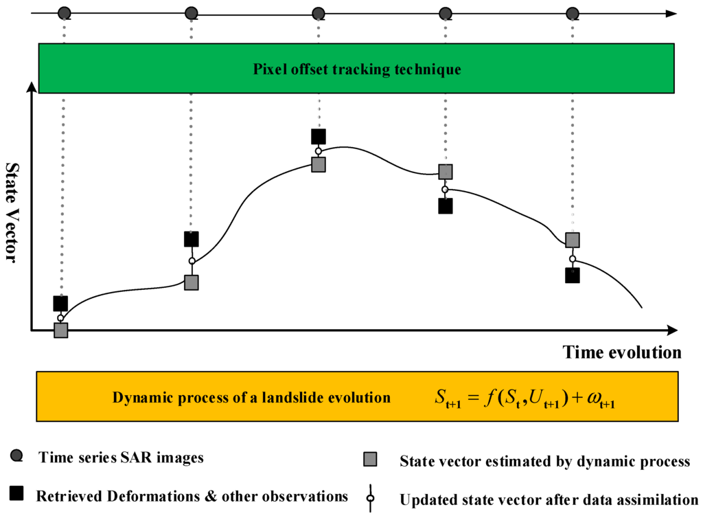
Figure 3.
The sequential data assimilation process for this study.
2.3.2. Framework of Ensemble Kalman Filter
The EnKF algorithm consists of three processes for each assimilation step: a forecast based on current state variables (i.e., solve landslide evolution equations with current static and dynamic parameters), data assimilation (computation of a Kalman gain), and updating the state variables and parameters.
Similar to Equation (1), the model forecast is executed in the EnKF for each ensemble member as follows:
where Ne is the number of ensemble members, is the component of the ith ensemble member forecast at time t+1, is the ith updated ensemble member at time t, is the ith perturbed forcing variables, and is independent white noise for the forecast mode, drawn from multi-normal distributions with zero mean and specified covariance Qt+1. At time t+1, the observation ensemble member can be written as,
where yt+1 is observation vector at time t+1; HSt+1 is the observation data calculated from the true state St+1, and is the noise term with zero mean and specified covariance Rt+1.
In the analysis step, the observations are perturbed by adding random perturbations and used for updating the state variation of each member. The update process can be expressed as,
where is the updated state vector after assimilation at time t+1, Kt+1 is the Kalman gain matrix determining the weight between the modeling and observation states in the assimilation process, is the forecasted background covariance matrix at time t+1; is the mean of Ne forecasted state vectors at time t+1.
Finally, the updated ensemble is figured out, of which we compute the mean to get the updated state vector which completes the process of data assimilation at time t+1. Then, the updated ensemble is iterated forward along with to repeat the entire process for the next time step.
3. Study Area and Test Datasets
3.1. Study Area
The Three Gorges Dam (TGD) in China is the largest hydropower project in the world. Since the Three Gorges Reservoir (TGR) went into operation in 2003, water level fluctuations have changed the physical and mechanical properties of rock and soil around the reservoir. The resulting ground deformation has re-activated previous landslides and created new landslide hazards [35]. Preconstruction landslide investigations for the TGD identified the Shuping landslide area as an old landslide that was re-activated during the first impoundment of the TGR [49].
The landslide is located in the Shuping Village of Zigui County on the south bank of the Yangtze River (Figure 1), approximately 49 km upstream of the Three Gorges Dam site [22,50]. The landslide extends into the Yangtze River and lies at an elevation between 65 and 400 m with a width of about 650 m. It is a south–north oriented landslide with a slope gradient varying from 22° in the upper part to 35° in the lower part. The landslide has an approximately 40–70 m thick sliding mass consisting of about 20 million m3 of sandy mudstone and muddy sandstone belonging to the Triassic Badong formation (T2b). Geological surveys show that landslides are likely to occur within this stratigraphic unit in the Three Gorges area [51,52].
From Figure 4 we can see that in the past, a valley has divided the Shuping landslide into eastern Block 1 and western Block 2 portions. Since 2005, 18 corner reflectors have been installed sparsely at Shuping landslide to help understand the landslide evolution [53,54], as presented in Figure 5. Out of the 18 corner reflectors, four (CR8, CR13, CR17, CR18) showed up only on images acquired after 24 January 2009. Among them, corner reflector CR12 is located on a stable area outside but adjoined to the landslide and thus was used as a reference point [50].
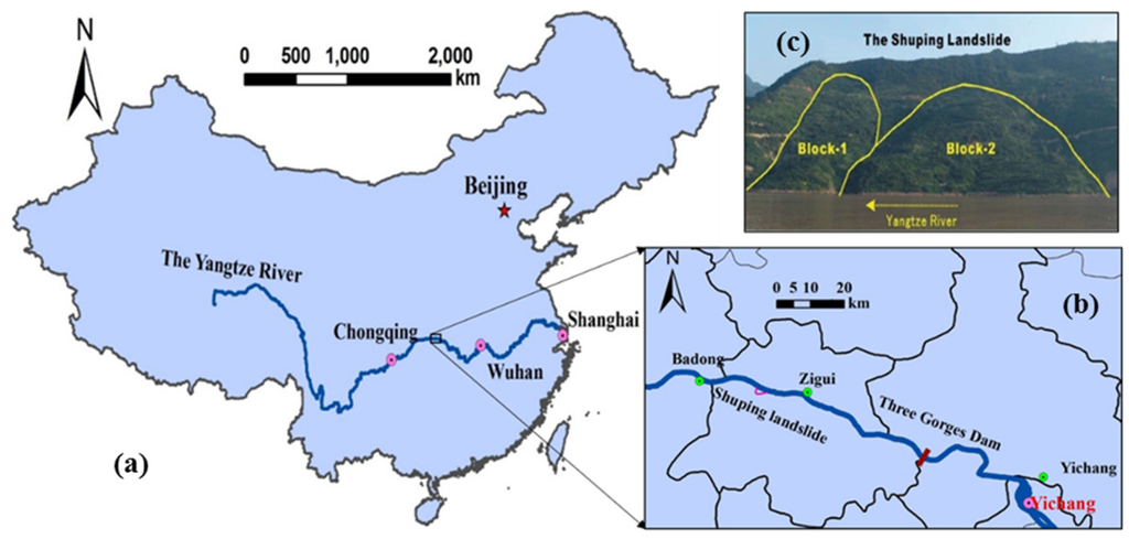
Figure 4.
Location of the Shuping landslide in China (a,b) and a photo of Shuping landslide taken from opposite bank facing south (c) [22].
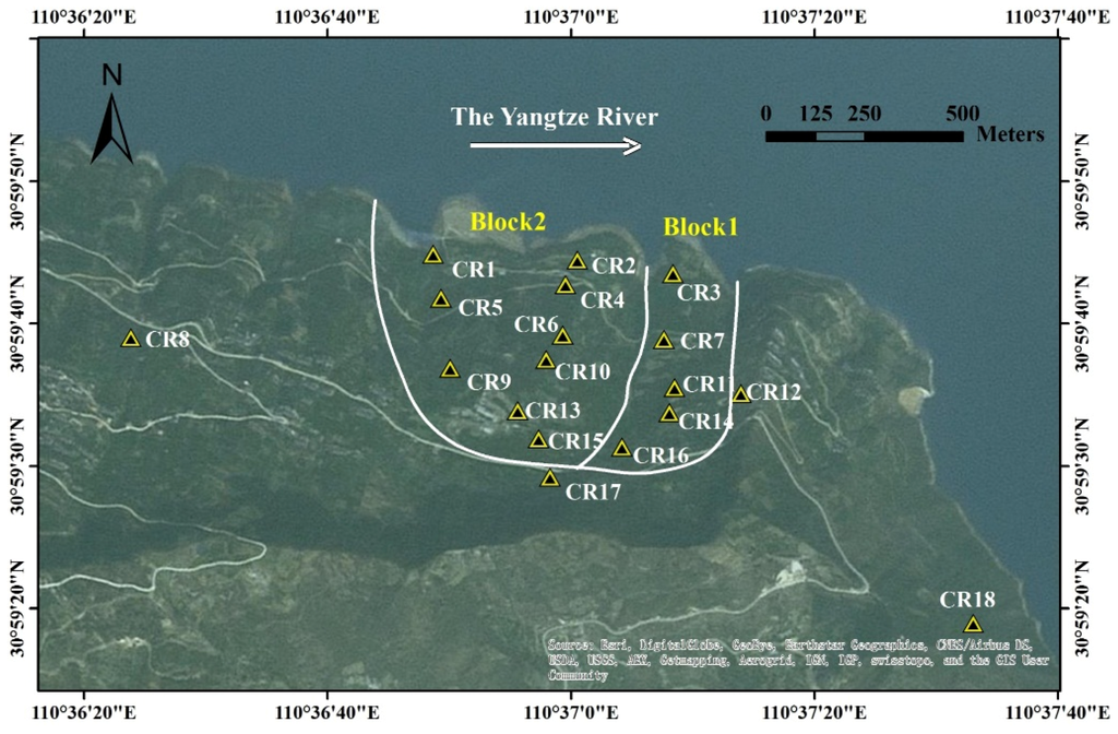
Figure 5.
The distribution of 18 corner reflectors at Shuping landslide.
The Three Gorges area belongs to a subtropical zone with a humid monsoon climate [55]. The average annual rainfall exceeds 1200 millimeters, concentrated between June and October. The Shuping landslide area is located in a precipitation area characterized by heavy rain and storms. Historic displacement measurements at Shuping using GPS and an extensometer indicated that the rate of the ground deformation increased with the drawdown of the reservoir level and during the period of increased rainfall in the wet season [4,35].
3.2. Datasets
In this study, we focus on Shuping landslide aiming to illustrate the suitability of data assimilation for understanding the interaction between landslide movements derived from POT and the influence of hydrological factors (i.e., reservoir water level and rainfall). For this purpose, four time-series datasets have been considered and analyzed. Two of them correspond to the displacement time-series of the landslide, which were measured by POT with TerraSAR-X StripMap (SM) and High Spotlight (HS) mode imageries. In addition, the other two correspond to the triggering factors, which are supposed to be related with the landslide deformation mechanism.
The basic parameters of the SAR images are shown in Table 1. The SAR monitoring results were obtained by processing 34 SM-mode and 36 HS-mode TerraSAR-X images through the POT approach. A detailed description of POT technology and data processing can be found in [22]. The measurements derived from the SM and HS dataset are two-dimensional in both azimuth and range direction.

Table 1.
Basic parameters about the TerraSAR-X images.
The daily reservoir water level was available for the period of June 2008 to May 2010. In November 2008, the TGR had become fully operational when its highest water level reached 175 m. Since then, reservoir water level fluctuates between 145 m and 175 m over the course of a year. These seasonal changes in water level exhibit clear seasonal changes due to artificial flood control [55,56].
Daily rainfall data are also available from the meteorological station at Badong in 2008 and Zigui between 2009 and 2010. The rainy season of Shuping landslide area lasts from June to October each year. The rainfall data in Figure 6 displays clear seasonal variations due to monsoon influences.
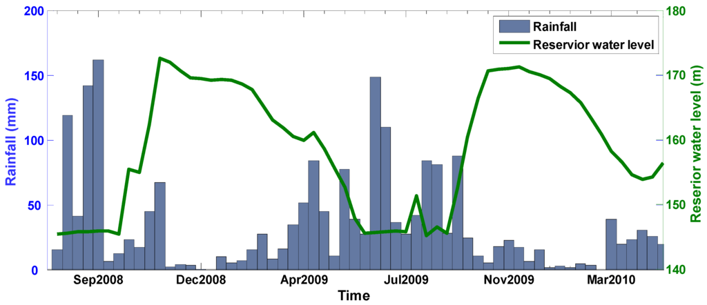
Figure 6.
The fluctuations of the synchronous reservoir water level and rainfall.
As can be seen from Figure 6, the water level fluctuated in a cycle opposite to the natural precipitation conditions. The reservoir began impounding at the end of the wet season in October and quickly reached the maximum water level and maintained this from November to February for power generation and navigation. Then, the reservoir water level was gradually decreased to the minimum previous level during spring, for flood control.
4. Experimental Results and Analyses
4.1. Deformation Characteristics of Shuping Landslide Area
As can be seen in Figure 7 and Figure 8, three CRs, namely CR8, CR17 and CR18 are located on a stable region outside the landslide area, and remained stable over a long period of nearly two years. The cumulative displacements derived from both HS and SM stacks are not more than 0.1 m. These results are reasonable and agree with the actual situation, which confirms the reliability of POT in deformation monitoring. The distribution of displacement derived from HS and SM data are almost identical in both azimuth and range at same locations, although the HS mode starting acquisition date was seven months later with a 15° difference in look angle compared to the SM mode.
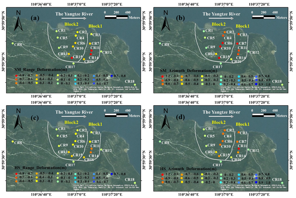
Figure 7.
Monitoring displacements from 21 July 2008 to 1 May 2010 using SM data in (a) range and (b) azimuth; Monitoring Displacements from 21 February 2009 to 15 April 2010 using HS data in (c) range and (d) azimuth.
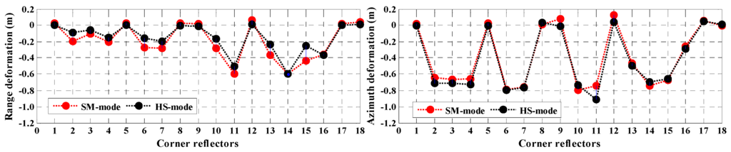
Figure 8.
Displacements of CRs at Shuping landslide in range (left) and azimuth (right) during February 2009 to April 2010. The black dot represents the SM-mode measurements, and the red dot represents the HS-mode measurements.
Also shown in Figure 7 and Figure 8, the spatial pattern of the measurements revealed that the deformation of the Shuping landslide varies with location. The deformation distribution of Block-1 was quite different with that of Block-2. The cumulative displacements at PTs within Block-1 are almost uniformly distributed with approximate meter-level displacements moving toward Yangtze River in azimuth. An approximate elevation-dependent displacement shows up as a large deformation near the upper part of Block-1, while an almost stable state near the lower part of Block-1 in range. In contrast, large displacements only show up in the eastern part of Block-2 neighboring Block-1, while there is a nearly stable state present in the western part of Block-2. The cumulative azimuth and range displacements at PTs within the eastern part of Block-2 are similar in spatial pattern to that of Block-1, implying that these two areas may share a similar deformation mechanism.
As shown in Table 2, the other fourteen corner reflectors installed at the slide are artificially categorized into three groups, considering their geographic locations and evolution features. The CR1, CR5 and CR9 corner reflectors located in the western part of Block-2 were assigned in group 1. As can be seen in Figure 7 and Figure 8, displacements in this group were 0.1 m at the most, from which it can be inferred that the western part of Block-2 was in a rather stable state from July 2008 to May 2010.
Table 2.
Groups of 18 corner reflectors.
The CR2, CR3, CR4, CR6, CR7 and CR10 corner reflectors near the upper part and the profile center of the landslide were denoted as Group 2; the CR11, CR13, CR14, CR15 and CR16 corner reflectors near the lower part of the landslide were marked as Group 3. These two groups experienced relatively significant displacement (Figure 7 and Figure 8) and exhibited similar temporal evolution features in both the azimuth and range during the study period, with similar abrupt displacements during April to June in 2009 (Figure 9). However, difference displacements still existed in the range direction between HS and SM measurements during the period February 2009 to June 2009. Such discrepancies are primarily caused by the big difference in look angle [22], since the range measurements has a cosine of the look angle relation with the vertical displacement. Consequently, when vertical displacement stays constant, a larger look angle (HS-mode) corresponds to a larger range deformation.
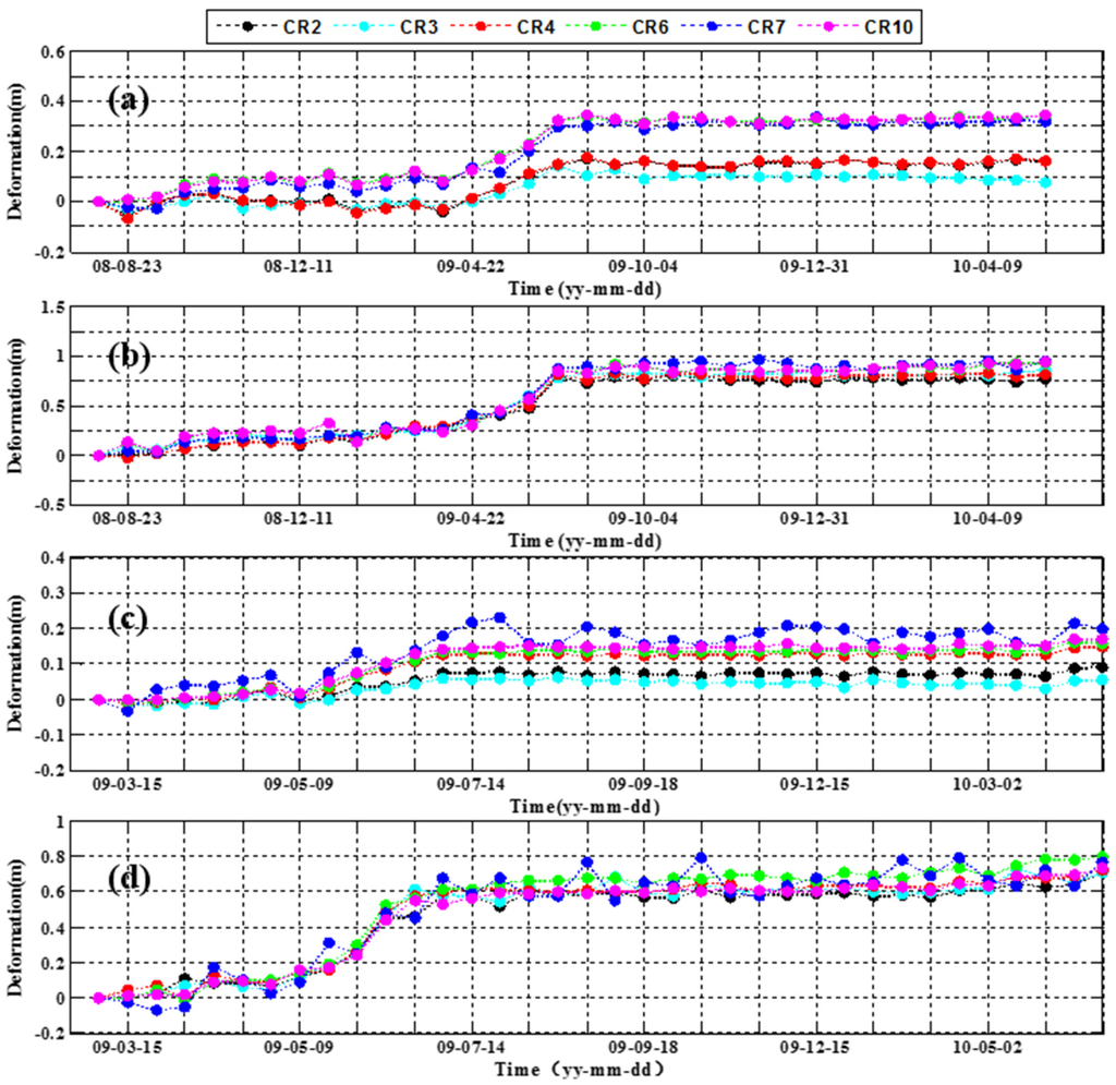
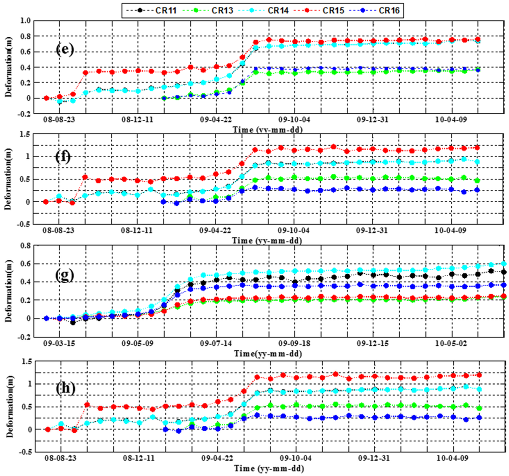
Figure 9.
Time-series displacement of corner reflectors in Groups 2 and 3. (a–d) are displacement at CRs in Group 2; (a,b) are displacement in range and azimuth using SM stack; (c,d) are displacement in range and azimuth using HS stack; (e–h) are displacement at CRs in Group 3; (e,f) are displacement in range and azimuth using SM stack; (g,h) are displacement in range and azimuth using HS stack.
The CRs in groups 2 and 3 show similar evolution features, two of the corner reflectors in Groups 2 and 3 were selected as the objects for analysis. One was CR2 located in the eastern part of Block-2, belonging to the upper part of the landslide, the other was CR14 installed in Block-1, belonging to the lower part of the landslide.
4.2. Time-Series Deformation Decomposition
As discussed in Section 2.2, the moving average method is the ideal method for eliminating the short-term uncertainty caused by random disturbances; however, it is a calculation from a moving window with 16 historical series observations, and infeasible for measurements from a HS stack, since it has only one complete cycle (approximately one cycle per year) from February 2009 to April 2010; otherwise, we could not obtain one complete period of the cyclical variation of displacement. Thus, AGO was adopted as an alternative to weaken the random disturbances from SAR derived displacements.
Displacement time-series at CR2 (in Block-2) and CR14 (in Block-1) derived from the SM dataset were used to estimate the feasibility of the AGO method in eliminating the randomness of the raw data. The de-noised displacements were separated into a trend and periodic components. The trend component was computed by a quadratic polynomial fitting method, while the seasonal component was calculated using the difference between the displacement time-series and the previously estimated trend component. The resulting deformation components were rendered in Figure 10 and Figure 11.
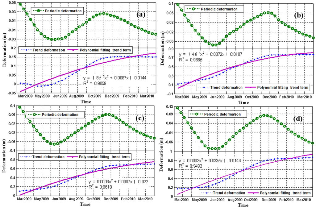
Figure 10.
The decomposition results of CR2 and CR14 using the moving average method; (a,b) are range and azimuth results of CR2; (c,d) are range and azimuth results of CR14.
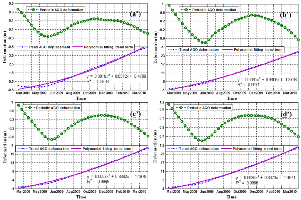
Figure 11.
The decomposition results of CR2 and CR14 using accumulated generating operation; (a’,b’) are range and azimuth results of CR2; (c’,d’) are range and azimuth results of CR14.
As can been in Figure 10a–d, the results from moving average method at CR2 and CR14 shared similar trends of both components’ evolution; as was the case using AGO method, shown in Figure 11a’–d’. These results are reasonable and confirm the stability of both methods in reducing short-term random disturbances whilst the calculated seasonal deformations at CR2 and CR14 using both methods had similar trends (also shown in Figure 10 and Figure 11) with minor discrepancies (Figure 12). However, because of the numerical sum of the AGO method, the derived results in Figure 11 are cumulative deformations, not the actual deformations at corner reflectors. As a result, the numerical values of both trend and periodic deformations were amplified many times as compared to those of the moving average method. For the trend component results from the AGO method, the magnitude depended on the time-series deformations of the corresponding corner reflectors, as shown in Figure 9. As for the periodic component, since it was controlled by the same seasonal changes of water level and rainfall, the amplitude of the fluctuation was uniform and approximately ten times the amplitude calculated using the moving average method, as can be seen in Figure 12.
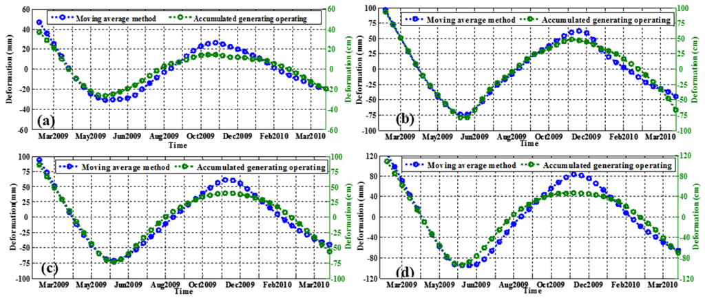
Figure 12.
A comparison of the calculated seasonal deformations between the moving average method and the accumulated generating operation method. Deformation time series in both range and azimuth were plot in (a,b) for CR2 and (c,d) for R14.
However, this different amplitude did not involve obstructions in subsequent processing, because we took the computation from the moving average method as a reference unit in the follow-up experiments. As a result, the AGO method could be used as an alternative and we compared it to the moving average method to make sure that AGO can be used to reduce short-term random disturbances. Even though AGO can be used as an alternative method, it still has disadvantages since it may smooth the peaks of the data, as shown in Figure 12. The moving average method can counteract the over-smoothing effect of AGO. Consequently, if sufficient data is available, the moving average method is recommended. Other methods, such as wavelet analysis in frequency domain, can certainly be considered to get rid of the short-term disturbance.
4.3. Impact Factors for Landslide Deformation
In Section 4.2, time-series decomposition was applied on two corner reflectors (CR2 and CR14) to extract the periodic displacement from the POT measurements. In this section, the periodic displacement of the CR14 corner reflector with severe fluctuation was chosen to analyze the relationship between the deformation and the causes.
We applied a grey relational analysis to determine the correlation between periodic deformation, water level and rainfall. The grey system theory proposed by Deng in 1982 [44] has been shown to be useful when dealing with incomplete and uncertain information. The grey relational analysis based on grey system theory can be effectively used to solve the complicated interrelationships among multiple performance characteristics [57]. Through grey relational analysis, one can obtain the grey relational degree to evaluate the correlation of different measurement data. The range of the relational degree value is −1 to 1; the closer the value to 1, the higher the correlation of two sequences. The calculated grey relational degrees are list in Table 3.
Table 3.
The correlation between periodic deformation and reservoir level as well as rainfall.
As can be seen in Table 3, the periodic component of the SAR time-series measurements was strongly correlated with reservoir level changes and seasonal precipitation. As shown in Figure 13, the periodic displacement fluctuated along with the variation of reservoir level and rainfall. It increased during the wet season with the water level remaining stable or rising, and decreased gradually with the reservoir level failing at the beginning of rainy season, indicating that the fluctuation of the reservoir water level was the major factor influencing deformation in the Shuping landslide area.
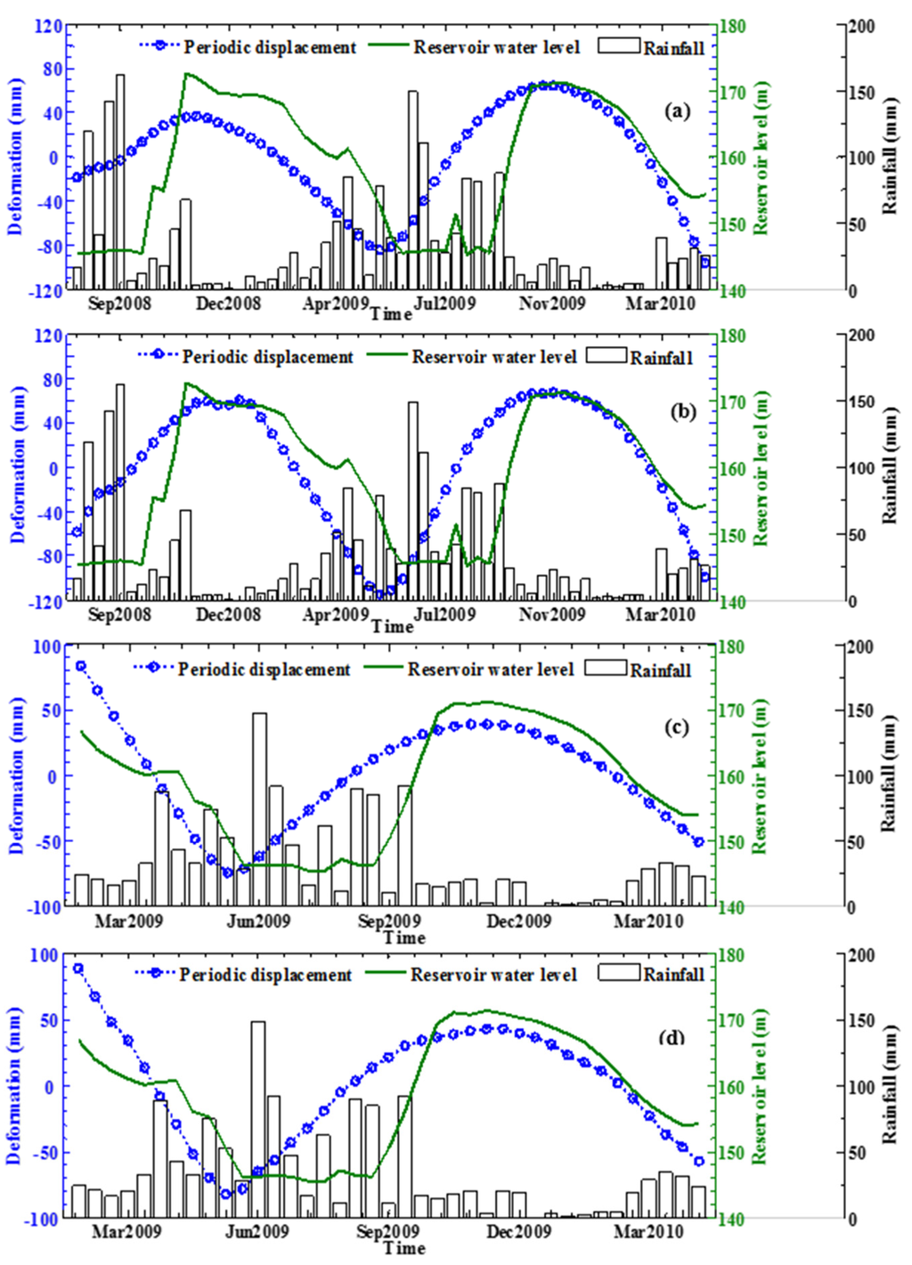
Figure 13.
The periodic component of the SAR time-series derived from SM mode data in range (a) and azimuth (b) and that from HS mode data in range (c) and azimuth (d).
In our previous study [22], we demonstrated that the total deformation was affected by the drawdown of the water level from April to June, but not by the sharp rise of the water level in October. From Figure 13, the water level rose rapidly from 145 m to 170 m during September to November both in 2008 and 2009. The change in deformation was very small, however, especially after excluding the effects of precipitation. Conversely, a very large deformation gradient occurred when the reservoir water fell quite rapidly from 170 m to 145 m in the period of November to April in both 2008 and 2009.
Since the rainy season of the Three Gorges area lasts from June to October, as can be seen in Figure 13, impacts of the rainfall on displacement appeared before the reservoir impoundment during the period of July 2008 to September 2008 and the period of June 2009 to September 2009. Larger periodic displacement occurred at the end of the rainy season when the reservoir water level had reached its highest in November 2008 and 2009. Combining these analyses, it is apparent that the fluctuation of reservoir water levels and rainfall were two significant triggering factors influencing the deformation in the Shuping landslide area.
4.4. Data Assimilation Results
Although the relationships among the rainfall, the water level, and landslide displacement were qualitatively analyzed in Section 4.3, a quantitative representation of this relationship needs further confirmation. The EnKF was adopted to validate the quantitative interactions of the Shuping landslide movement under the influence of hydrological factors.
The measured deformations are available at an interval of 11 days, during this short time-step, the variation of the periodic displacement was very small. Thus, the fluctuation of the periodic motion can be perceived as smooth, as shown in Figure 13. With this in mind, we considered periodic displacement to be a function of the water level and rainfall. Thus, a Taylor series expansion could be applied. The dynamic equation of periodical deformation can be expressed as:
where d is the periodic motion, wt and rt is the reservoir water level and rainfall at time t respectively, , , , and are the first and second partial derivatives of periodic displacement versus water level w and rainfall r, g is the third order or higher remainder term of the Taylor expansion with a small value. In quantitative terms, the effects of the trigging factors are not comparable because of different units of measurement and dimensions. To eliminate the effect of the index dimension, Min-Max Normalization was carried out [58].
In this study, the ensemble number Ne was set to 1000; the standard deviation g was scaled with a scaling factor of 10% multiplied to the current forecast values. Since, , , , and are partial derivatives, we could not accurately estimate certain values. Thus, we take these four partial values as model parameters in the state vector and updated them synchronously during assimilation. Based on these parameter settings and those discussed in Section 2.2, the model iteratively ran through the time-steps in sequence while being assimilated to the water level and rainfall observations.
The assimilation and simulation results after the parameters were optimized for the periodic motion of the CR14 corner reflector in both range and azimuth from February 2009 to April 2010 are shown in Figure 14. These figures show that, as the assimilation is progressing, the data assimilation estimates provided good representation of the SAR derived displacements and the optimized parameter simulation results become more reliable than the testing results after running a few steps. The mean absolute error of the assimilation results were shown in Figure 14. We can see that at the beginning of data assimilation, the estimation error of EnKF was relatively high with maximum error at approximately 25 mm, but, after a few steps forward, it decreased gradually. However, it could not reach zero due to either the incomplete parameters or the observation errors already incorporated in the dynamic process.
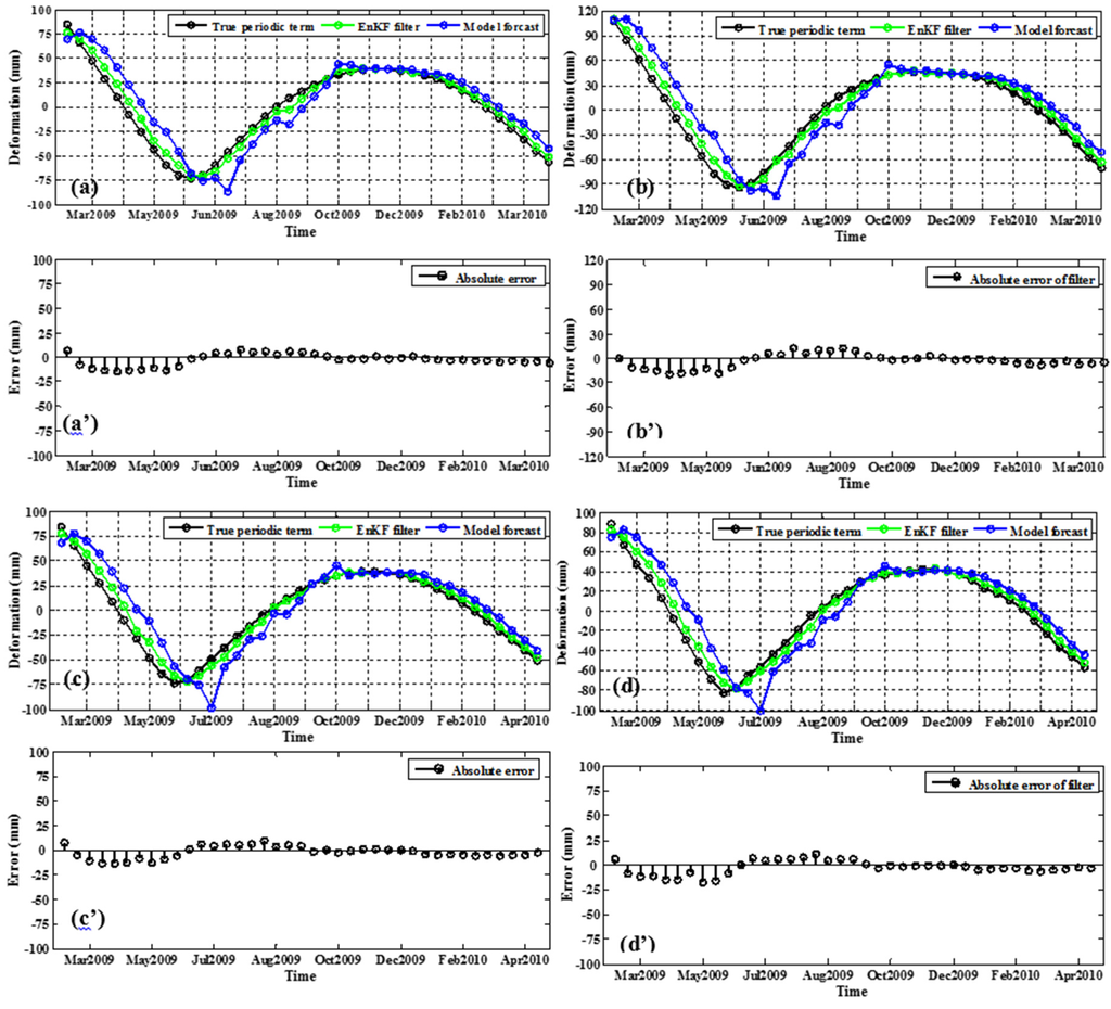
Figure 14.
The assimilation results and their corresponding mean absolute error of periodic motion at point CR14 from February 2009 to April 2010; among them (a,b) were assimilation and simulation results from SM mode stack in range and azimuth separately with (a’,b’) as the corresponding mean absolute error; (c,d) were assimilation and simulation results from HS mode stack in range and azimuth separately with (c’,d’) as the corresponding mean absolute error.
Since the four parameters used in the dynamic equation were synchronously optimized by assimilation observations during the data assimilation process. This allowed the predictive uncertainties of the periodical deformation to be reduced. In this study, data assimilation progressed until finishing assimilation the observations acquired on 20 April 2009 and 15 April 2009 for SM- and HS-mode series. Then, we adopted the updated model parameters to make a short term forecast for the periodic term displacement. As can been seen in Table 4, the short term forecasts are consistent with our analysis of the relationship between the deformation and the impact factors in Section 4.3. In concrete terms, the hydrologic conditions of the Shuping landslide area are as follows: the water level of TGR remains low during the period from May to September and the rainy season in the Three Gorges area does not begin until June. Consequently, in May, the corresponding displacement variation affected by the fluctuation of water level and rainfall reduces to the lowest value; that is to say, the periodic motion of CR14 falls to the lowest level in May. Conversely, with the commencement of the rainy season in June, a gradual increase of the periodic displacement occurred. As can be seen in Table 4, although the results from the two stacks do not strictly align in terms of timing, these results are consistent with the developing trend, which suggests the feasibility of data assimilation for studying the combined effects of presumed triggering factors on landslide deformation. Considering that we placed the uncertain parameters of the model into the state vector to synchronize updates, this approach relies on state-parameter dependencies and is not able to provide good estimates if the dependencies are weak. To address this challenge, novel variants of the EnKF, such as dual estimate approaches [59], may be useful remedies.
Table 4.
A short term forecast of the periodic term displacement.
Results confirm that EnKF is suitable for landside research. It can continually update landside states and model parameters when new data become available. Recently, the EnKF has become popular in many areas of the earth sciences because it is easy to use, is flexible, and has relatively few restrictive assumptions [19,21]. However, the potential of EnKF in landside disaster research needs further exploration to address ongoing issues in the coupling mode between the landslide observations (including the in situ measurements and remote sensing retrieval data) and other mechanism models (e.g., Transient Rainfall Infiltration and Grid-based Regional Slope-Stability Model (TRIGRS) and in the Fast Lagrangian Analysis of Continua model (FLAC3D)). If these issues are settled, then this method could assist in disaster early-warning systems and forecasting.
In specific applications, the success of data assimilation is quite dependent on the error specification in the model, error in observations, and the ensemble size. When designing the data assimilation scheme, EnKF requires error estimations of the dynamic process and error estimation for the observations to properly couple model predictions with observations. However, it is very difficult to quantify these errors because the sources and statistical structure of each error are often unknown. In this study, we assumed that larger value variables could introduce larger errors; thus, the error noises were represented by adding a scaling factor to the then-current values of the variable. In actual applications, it is preferable to overestimate rather than underestimate errors as the underestimation may result in filter divergences. However, a much larger bias would make the system unstable and propagate improper information to the next time step, thus spoiling assimilation performance. The ensemble is a set of realizations in the EnKF and used to approximate the probability distribution of the state variables. Generally, enlarging the ensemble size enables the EnKF to propagate the error information more accurately; however, at the same time, it increases the computational burden. Consequently, if there is no calculation burden, we prefer a larger ensemble size (e.g., 1000) to get a more accurate result; or if a large complex model is adopted in the assimilation scheme, we have to make a compromise between estimation accuracy and computational feasibility.
5. Conclusions
In recent years, time-series SAR techniques have been successfully applied to detect landslide deformation. However, most of these studies focused primarily on technical innovation and applications. Few studies have considered the further interpretation of SAR/InSAR derived landslide displacements in relation to potential triggering factors, although this work is of crucial importance to understand deformation mechanisms and assist disaster early-warning and forecasting.
In this study, we executed a coupled analysis based on data assimilation methodology to explore the displacement response in the Shuping landslide area under the influence of hydrological factors. Corner reflectors installed at/near the landslide zone were utilized in the Pixel Offset Tracking (POT) technique to analyze the spatial-temporal evolution of landslide deformation. The measurements with SM- and HS-mode TerraSAR-X imageries showed consistency in their spatial-temporal patterns. Because the corner reflectors usually maintain very high coherence (>0.8), the achievable accuracy can reach cm-level.
Since the reservoir water level and rainfall are the primary causes of displacement fluctuations, they can be regarded as periodic displacement. Therefore, we performed time-series decomposition on the POT monitoring results to obtain the periodic displacement. Our seasonal deformation results showed that the AGO can be used as an alternative method to weaken the random disturbance from SAR derived displacements. However, if sufficient data is available, the moving average method is preferable. Then, a grey relational analysis was conducted to estimate the grey relational degree between the periodic displacement and the inducing factors.
We adopted a sequential data assimilation method named EnKF to study the quantitative interactions of the landslide movement under the influence of hydrological factors. By incorporating available observations sequentially in time, the variables and parameters used in dynamic equations were synchronously optimized, the resulting assimilated estimates matched well with the SAR derived displacements while the predictive uncertainties were reduced over time. The predictions of periodic displacement for SM- and HS-mode time-series were compared and analyzed with the seasonal variation of the trigging factors. These results showed similarities with developing trends and were consistent with variation of the trigging factors.
Preliminary results confirmed that the EnKF is feasible for studying the deformation response mechanisms of landslide areas near a reservoir under the influence of hydrological factors. To facilitate the success of data assimilation processing, error specification must be consistent with the model capability and the measurement flexibility. We propose the EnKF sequential data assimilation method as a possible approach to get an accurate estimation of a current landslide state and generate prognostic variables for landslide evolution, which are of particular importance for disaster forecasting and developing early warning systems.
As the triggering factors of rainfall episodes and reservoir water levels continue to change, the variation in the Shuping landslide kinematics will also continue over time. Though the current deformation may not have a devastating impact, significant deformation showed up in Block-1 and the eastern part of Block-2. The maximum cumulative deformation exceeded 1 m during the period of July 2008 to May 2009. In contrast, a rather stable state was identified in the western part of Block-2. Therefore, the landslide deformation monitoring with mechanism analysis is a vital tool for understanding the further progress of the landslides and subsequently developing early hazard warning systems. Further studies will be followed by combining multi-track SAR data to derive the three-dimensional displacement fields for the Shuping landslide area, since they are favored by geologists when investigating earth surface deformation mechanisms.
Acknowledgments
This work is financially supported by the National Key Basic Research Program of China (Grant No. 2013CB733205 and Grant No. 2013CB733204). The authors would like to thank the Astrium Satellite Company and the German Aerospace Center (DLR) for providing the TerraSAR-X datasets through the General AO project (GEO0606) and TSX-Archive-2012 AO project (GEO1856).
Author Contributions
Yanan Jiang implemented the methodology and finished the manuscript organization. Mingsheng Liao supervised and guided the research. Zhiwei Zhou and Lu Zhang provided valuable suggestions for the revision. Xuguo Shi and Lu Zhang modified the Pixel Offset Tracking algorithm for this study. All authors contributed extensively with writing this paper.
Conflicts of Interest
The authors declare no conflict of interest.
References
- Au, S.W.C. Rain-induced slope instability in Hong Kong. Eng. Geol. 1998, 51, 1–36. [Google Scholar] [CrossRef]
- Schuster, R.L.; Highland, L. Socioeconomic and Environmental Impacts of Landslides in the Western Hemisphere; U.S. Geological Survey (Citeseer): Denver, CO, USA, 2001.
- Huang, R.Q. Some catastrophic landslides since the twentieth century in the southwest of China. Landslides 2009, 6, 69–81. [Google Scholar]
- Wang, F.W.; Zhang, Y.M.; Huo, Z.T.; Peng, X.M.; Araiba, K.; Wang, G.H. Movement of the shuping landslide in the first four years after the initial impoundment of the Three Gorges Dam reservoir, China. Landslides 2008, 5, 321–329. [Google Scholar] [CrossRef]
- Crosta, G.; Frattini, P.; Agliardi, F. Deep seated gravitational slope deformations in the European Alps. Tectonophysics 2013, 605, 13–33. [Google Scholar] [CrossRef]
- Michoud, C.; Baumann, V.; Lauknes, T.; Penna, I.; Derron, M.H.; Jaboyedoff, M. Large slope deformations detection and monitoring along shores of the Potrerillos Dam reservoir, argentina, based on a small-baseline InSR approach. Landslides 2015, 4. [Google Scholar] [CrossRef]
- Liu, C.Z.; Liu, Y.H.; Wen, M.S.; Li, T.F.; Lian, J.F.; Qin, S.W. Geo-hazard initiation and assessment in the Three Gorges reservoir. In Landslide Disaster Mitigation in Three Gorges Reservoir, China; Springer: Berlin, Germany, 2009; pp. 3–40. [Google Scholar]
- Ferretti, A.; Prati, C.; Rocca, F. Permanent scatterers in SAR interferometry. IEEE Trans. Geosci. Remote. Sens. 2001, 39, 8–20. [Google Scholar] [CrossRef]
- Berardino, P.; Fornaro, G.; Lanari, R.; Sansosti, E. A new algorithm for surface deformation monitoring based on small baseline differential SAR interferograms. IEEE Trans. Geosci. Remote. Sens. 2002, 40, 2375–2383. [Google Scholar] [CrossRef]
- Arnaud, A.; Adam, N.; Hanssen, R.; Inglada, J.; Duro, J.; Closa, J.; Eineder, M. ASAR-ERS interferometric phase continuity. In Proceedings of the IEEE International Geoscience and Remote Sensing Symposium, Toulouse, France, 21–25 July 2003; pp. 1133–1135.
- Werner, C.; Wegmüller, U.; Strozzi, T.; Wiesmann, A. Interferometric point target analysis for deformation mapping. In Proceedings of the IEEE International Geoscience and Remote Sensing Symposium, Toulouse, France, 21–25 July 2003; pp. 4362–4364.
- Blanco-Sanchez, P.; Mallorquí, J.J.; Duque, S.; Monells, D. The Coherent Pixels Technique (CPT): An advanced DInSAR technique for nonlinear deformation monitoring. Pure Appl. Geophys. 2008, 165, 1167–1193. [Google Scholar] [CrossRef]
- Ferretti, A.; Fumagalli, A.; Novali, F.; Prati, C.; Rocca, F.; Rucci, A. A new algorithm for processing interferometric data-stacks: SqueeSAR. IEEE Trans. Geosci. Remote. Sens. 2011, 49, 3460–3470. [Google Scholar] [CrossRef]
- Strozzi, T.; Luckman, A.; Murray, T.; Wegmüller, U.; Werner, C.L. Glacier motion estimation using SAR offset-tracking procedures. IEEE Trans. Geosci. Remote. Sens. 2002, 40, 2384–2391. [Google Scholar] [CrossRef]
- Notti, D.; Calò, F.; Cigna, F.; Manunta, M.; Herrera, G.; Berti, M.; Meisina, C.; Tapete, D.; Zucca, F. A user-oriented methodology for DInSAR time series analysis and interpretation: Landslides and subsidence case studies. Pure Appl. Geophys. 2015, 172, 3081–3105. [Google Scholar] [CrossRef]
- Tomás, R.; Li, Z.; Liu, P.; Singleton, A.; Hoey, T.; Cheng, X. Spatiotemporal characteristics of the Huangtupo landslide in the Three Gorges region (China) constrained by radar interferometry. Geophys. J. Int. 2014, 197, 213–232. [Google Scholar] [CrossRef]
- Daley, R. Atmospheric Data Analysis, Cambridge Atmospheric and Space Science Series; Cambridge University Press: Cambridge, UK, 1991. [Google Scholar]
- Talagrand, O. Assimilation of observations, an introduction. J. Meteorol. Soc. Jpn. 1997, 75, 81–99. [Google Scholar]
- Evensen, G. Data Assimilation—The Ensemble Kalman Filter, 2nd ed.; Springer: Berlin, Germany, 2009. [Google Scholar]
- Huang, C.L.; Li, X.; Lu, L.; Gu, J. Experiments of one-dimensional soil moisture assimilation system based on Ensemble Kalman filter. Remote Sens. Environ. 2008, 112, 888–900. [Google Scholar] [CrossRef]
- Xie, X.H.; Zhang, D.X. Data assimilation for distributed hydrological catchment modeling via ensemble kalman filter. Adv. Water Resour. 2010, 33, 678–690. [Google Scholar] [CrossRef]
- Shi, X.G.; Zhang, L.; Balz, T.; Liao, M.S. Landslide deformation monitoring using point-like target offset tracking with multi-mode high-resolution TerraSAR-X data. ISPRS J. Photogramm. 2015, 105, 128–140. [Google Scholar] [CrossRef]
- Wang, L. Research of Recurrence Mechanism and Prediction of Shuping Landslide under Water Level Variation and Rainfall in Three Gorges Reservoir Area. Master’s Thesis, China Three Gorges University, Yichang, China, 15 May 2014. [Google Scholar]
- Ren, F.; Wu, X.L.; Zhang, K.X.; Niu, R.Q. Application of wavelet analysis and a particle swarm-optimized support vector machine to predict the displacement of the shuping landslide in the Three Gorges, China. Environ. Earth Sci. 2015, 73, 4791–4804. [Google Scholar] [CrossRef]
- Peng, L.; Niu, R.Q.; Wu, T. Time series analysis and support vector machine for landslide displacement prediction. J. Zhejiang Univ. 2013, 47, 1672–1679. [Google Scholar]
- Zhang, J.; Yin, K.L.; Wang, J.J.; Huang, F.M. Diaplacement prediction of baishuihe landslide based on time series and pso-svr model. Chin. J. Rock Mech. Eng. 2015, 34, 382–391. [Google Scholar]
- Carnec, C.; Massonnet, D.; King, C. Two examples of the application of SAR interferomety to sites of small extent. Geophys. Res. Lett. 1996, 23, 3579–3582. [Google Scholar] [CrossRef]
- Berardino, P.; Costantini, M.; Franceschetti, G.; Iodice, A.; Pietranera, L.; Rizzo, V. Use of differential SAR interferometry in monitoring and modelling large slope instability at maratea (Basilicata, Italy). Eng. Geol. 2003, 68, 31–51. [Google Scholar] [CrossRef]
- Catani, F.; Farina, P.; Moretti, S.; Nico, G.; Strozzi, T. On the application of SAR interferometry to geomorphological studies: Estimation of landform attributes and mass movements. Geomorphology 2005, 66, 119–131. [Google Scholar] [CrossRef]
- Lauknes, T.R.; Piyush Shanker, A.; Dehls, J.F.; Zebker, H.A.; Henderson, I.H.C.; Larsen, Y. Detailed rockslide mapping in northern norway with small baseline and persistent scatterer interferometric SAR time series methods. Remote Sens. Environ. 2010, 114, 2097–2109. [Google Scholar] [CrossRef]
- Massonnet, D.; Feigl, K.L. Radar interferometry and its application to changes in the earth’s surface. Rev. Geophys. 1998, 36, 441–500. [Google Scholar] [CrossRef]
- Bianchini, S.; Herrera, G.; Mateos, R.; Notti, D.; Garcia, I.; Mora, O.; Moretti, S. Landslide activity maps generation by means of Persistent Scatterer interferometry. Remote Sens. 2013, 5, 6198–6222. [Google Scholar] [CrossRef]
- Liu, P.; Li, Z.H.; Hoey, T.; Kincal, C.; Zhang, J.F.; Zeng, Q.M.; Muller, J.-P. Using advanced InSAR time series techniques to monitor landslide movements in badong of the three gorges region, China. Int. J. Appl. Earth Obs. 2013, 21, 253–264. [Google Scholar] [CrossRef]
- Raspini, F.; Moretti, S.; Casagli, N. Landslide mapping using SqueeSAR data: Giampilieri (Ialy) case study. In Landslide Science and Practice; Springer: Berlin, Germany, 2013; Volume 1, pp. 147–154. [Google Scholar]
- Singleton, A.; Li, Z.; Hoey, T.; Muller, J.-P. Evaluating sub-pixel offset techniques as an alternative to D-InSAR for monitoring episodic landslide movements in vegetated terrain. Remote Sens. Environ. 2014, 147, 133–144. [Google Scholar] [CrossRef]
- Fan, J.H.; Lin, H.; Xia, Y.; Zhao, H.L.; Guo, X.F.; Li, M. Mapping the deformation of shuping landslide using DInSAR and offset tracking methods. In Landslide Science for a Safer Geoenvironment; Sassa, K., Canuti, P., Yin, Y., Eds.; Springer: Berlin, Germany, 2014; pp. 319–324. [Google Scholar]
- Raspini, F.; Ciampalini, A.; del Conte, S.; Lombardi, L.; Nocentini, M.; Gigli, G.; Ferretti, A.; Casagli, N. Exploitation of amplitude and phase of satellite SAR images for landslide mapping: The case of montescaglioso (south Italy). Remote Sens. 2015, 7, 14576–14596. [Google Scholar] [CrossRef]
- Sansosti, E.; Berardino, P.; Bonano, M.; Calò, F.; Castaldo, R.; Casu, F.; Manunta, M.; Manzo, M.; Pepe, A.; Pepe, S. How second generation SAR systems are impacting the analysis of ground deformation. Int. Appl. Earth Obs. 2014, 28, 1–11. [Google Scholar] [CrossRef]
- Hu, X.; Wang, T.; Liao, M.S. Measuring coseismic displacements with point-like targets offset tracking. IEEE Geosci. Remote Sens. 2014, 11, 283–287. [Google Scholar] [CrossRef]
- Li, X.F.; Muller, J.P.; Fang, C.; Zhao, Y.H. Measuring displacement field from TerraSAR-X amplitude images by subpixel correlation: An application to the landslide in Shuping, Tree Grges area. Acta Petrol. Sin. 2011, 27, 3843–3850. [Google Scholar]
- Seng, H.S. A new approach of moving average method in time series analysis. In Proceedings of the New Media Studies (CoNMedia), Tangerang, Indonesia, 27–28 November 2013; pp. 1–4.
- Xu, F.; Wang, Y.; Du, J.; Ye, J. Study of displacement prediction model of landslide based on time series analysis. Chin. J. Rock Mech. Eng. 2011, 30, 746–751. [Google Scholar]
- Kayacan, E.; Ulutas, B.; Kaynak, O. Grey system theory-based models in time series prediction. Expert Syst. Appl. 2010, 37, 1784–1789. [Google Scholar] [CrossRef]
- Deng, J.L. Control problems of grey systems. Syst. Control Lett. 1982, 1, 288–294. [Google Scholar]
- Evensen, G. Sequential data assimilation with a nonlinear quasi-geostrophic model using Monte Carlo methods to forecast error statistics. J. Geophys. Res. 1994, 99, 10143. [Google Scholar] [CrossRef]
- Burgers, G.; van Jan Leeuwen, P.; Evensen, G. Analysis scheme in the ensemble Kalman filter. Mon. Weather Rev. 1998, 126, 1719–1724. [Google Scholar] [CrossRef]
- Van Leeuwen, P.J. Comment on data assimilation using an ensemble kalm$an filter technique. Mon. Weather Rev. 1999, 127, 1374–1377. [Google Scholar] [CrossRef]
- De Zan, F. Accuracy of Incoherent Speckle Tracking for Circular Gaussian Signals. IEEE Geosci. Remote Sens. 2014, 11, 264–267. [Google Scholar] [CrossRef]
- Chen, D.; Xue, G.; Xu, F. Study on the Engineering Geology Properties in Three Gorges; Hubei Science and Technology Publisher: Wuhan, China, 1997. [Google Scholar]
- Fu, W.X.; Guo, H.D.; Tian, Q.J.; Guo, X.F. Landslide monitoring by corner reflectors differential interferometry SAR. Int. J. Remote Sens. 2010, 31, 6387–6400. [Google Scholar] [CrossRef]
- Wen, B.P.; Wang, S.J.; Wang, E.Z.; Zhang, J.M. Characteristics of rapid giant landslides in China. Landslides 2004, 1, 247–261. [Google Scholar] [CrossRef]
- Wang, F.W.; Zhang, Y.M.; Huo, Z.T.; Peng, X.M. Monitoring on shuping landslide in the Three Gorges Dam Reservoir, China. In Landslide Disaster Mitigation in Three Gorges Reservoir, China; Springer: Berlin, Germany, 2009; pp. 257–273. [Google Scholar]
- Xia, Y. Synthetic aperture radar interferometry. In Sciences of Geodesy-I; Springer: Berlin, Germany, 2010; pp. 415–474. [Google Scholar]
- Xia, Y.; Kaufmann, H.; Guo, X.F. Landslide monitoring in the Three Gorges area using D-InSAR and corner reflectors. Photogramm. Eng. Remote Sens. 2004, 70, 1167–1172. [Google Scholar]
- Tomás, R.; Li, Z.; Lopez-Sanchez, J.M.; Liu, P.; Singleton, A. Using wavelet tools to analyse seasonal variations from InSAR time-series data: A case study of the Huangtupo landslide. Landslides 2015, 6. [Google Scholar] [CrossRef]
- Tullos, D. Assessing the influence of environmental impact assessments on science and policy: An analysis of the Three Gorges project. J. Environ. Manag. 2009, 90, S208–S223. [Google Scholar] [CrossRef] [PubMed]
- Lin, J.L.; Lin, C.L. The use of the orthogonal array with grey relational analysis to optimize the electrical discharge machining process with multiple performance characteristics. Int. J. Mach. Tools Manuf. 2002, 42, 237–244. [Google Scholar] [CrossRef]
- Li, X.Z.; Kong, J.M. Application of GA-SVM method with parameter optimization for landslide development prediction. Nat. Hazards Earth Syst. 2014, 14, 525–533. [Google Scholar] [CrossRef]
- Yang, K.; Koike, T.; Kaihotsu, I.; Qin, J. Validation of a dual-pass microwave land data assimilation system for estimating surface soil moisture in semiarid regions. J. Hydrometeorol. 2009, 10, 780–793. [Google Scholar] [CrossRef]
© 2016 by the authors; licensee MDPI, Basel, Switzerland. This article is an open access article distributed under the terms and conditions of the Creative Commons by Attribution (CC-BY) license (http://creativecommons.org/licenses/by/4.0/).