Abstract
The goal of the paper is to detect pixels that contain targets of known spectra. The target can be present in a sub- or above pixel. Pixels without targets are classified as background pixels. Each pixel is treated via the content of its neighborhood. A pixel whose spectrum is different from its neighborhood is classified as a “suspicious point”. In each suspicious point there is a mix of target(s) and background. The main objective in a supervised detection (also called “target detection”) is to search for a specific given spectral material (target) in hyperspectral imaging (HSI) where the spectral signature of the target is known a priori from laboratory measurements. In addition, the fractional abundance of the target is computed. To achieve this we present two linear unmixing algorithms that recognize targets with known (given) spectral signatures. The CLUN is based on automatic feature extraction from the target’s spectrum. These features separate the target from the background. The ROTU algorithm is based on embedding the spectra space into a special space by random orthogonal transformation and on the statistical properties of the embedded result. Experimental results demonstrate that the targets’ locations were extracted correctly and these algorithms are robust and efficient.
1. Introduction
1.1. Data Representation and Extraction of Spectral Information
Hyperspectral remote sensing exploits the fact that all materials reflect, absorb and emit electromagnetic energy at specific wavelengths. In comparison to a typical camera that uses red, green and blue colors as three wavelength bands, hyperspectral imaging (HSI) sensors acquire digital images in many contiguous and very narrow spectral bands that typically span the visible, near-infrared and mid-infrared portions of the spectrum. This enables to construct essentially continuous radiance spectrum for every pixel in the scene. The goal of the paper is to identify and classify materials that are present in HSI and to detect targets of interest.
Material and object detection using remotely sensed spectral information has many military and civilian applications. Detection algorithms can be divided into two classes: supervised and unsupervised. The unsupervised detection is also called “anomaly detection”. Anomalies are defined as patterns in the data that do not conform to a well defined notion of normal data behavior. In anomaly detection tasks, hyperspectral pixels have to be classified as either background (normal behavior) or anomalies. Every pixel or group of pixels, which are spectrally different in a meaningful way from the abundant (background) spectral material, are classified as anomalies. A survey of unsupervised detection algorithms is given in [1].
In a supervised detection (also called “target detection”), the main objective is to search for a specific given spectral material (target) in HSI. The spectral signature of the target is known a priori from laboratory measurements. In this paper, we focus on supervised target detection in HSI.
The paper has the following structure. Problem statement including HSI descriptions, which are used for testing the proposed algorithms, are given in Section 2. Related work are described in Section 3. Section 4 describes the needed mathematical background that is used for the constructed solution. Section 5 presents the ROTU algorithm that is based on orthogonal rotations. Classification for an unmixing algorithm is given in Section 6 and its experimental results are presented in Section 6.4.
2. Problem Statement
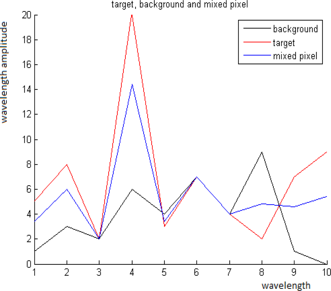
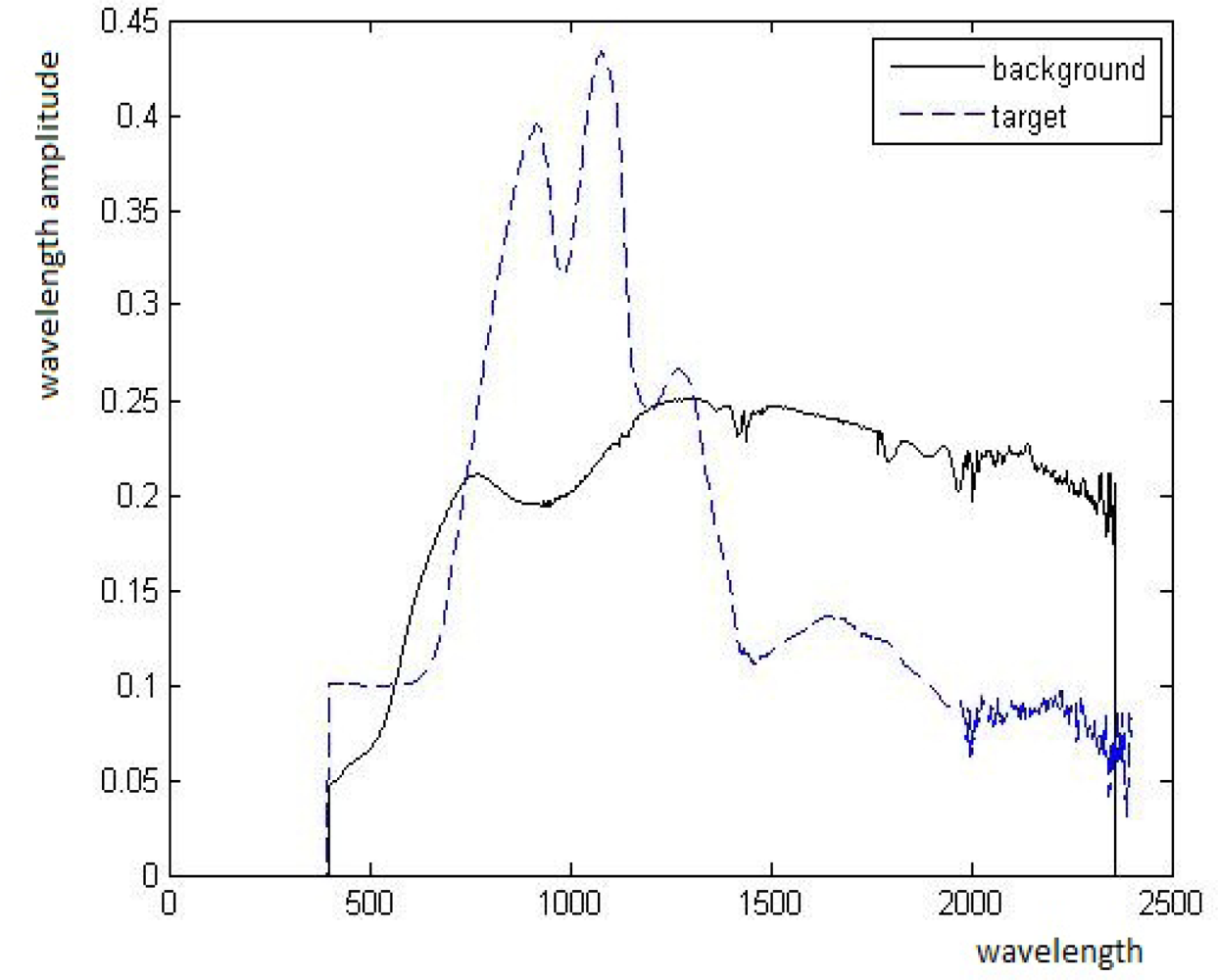
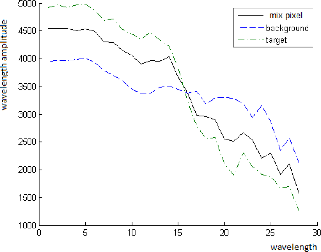
The goal in this paper is to detect pixels that contain targets of a known spectrum. The target can be present in a sub- or in a whole pixel. Pixels without targets are classified as background pixels. Each pixel is treated via the content of its neighborhood. A pixel whose spectrum is different from its neighborhood according to [2] is classified as a “suspicious point”. In each suspicious point there is a mix of target(s) and background. For example, Figures 1 and 2 display a scene from 2nd figure in Section 2.1 with an exemplary point. The background, the target and the mixed pixel spectra are displayed in Figure 3.
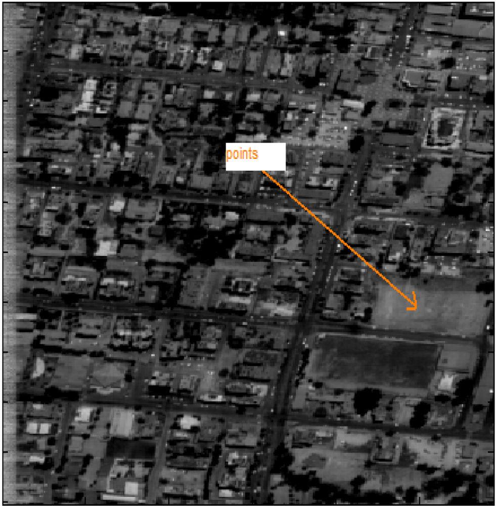
Figure 1.
Exemplary points that were taken from the area pointed by the arrow (full image is given in 2nd figure in Section 2.1).
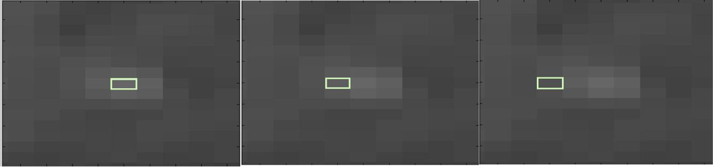
Figure 2.
Zoom on the exemplary point in Figure 1. Left: The marked pixel contains the target with the spectrum T as a whole pixel. Center: The marked pixel is a mixed pixel with the spectrum P. Right: The marked pixel is a pure background pixel with the spectrum B.
Linear mixing is the most widely used as spectral mixing model, which assumes that the observed reflectance spectrum of a given pixel is generated by a linear combination of a small number of unique constituent deterministic spectral signatures. Endmembers are the outputs from the spectral unmixing. This model is defined with constraints in the following way:
where s1, s2, . . . , sM are the M endmembers spectra which are assumed to be linearly independent, a1, a2, . . . , aM are the corresponding abundances (cover the material fractions) and w is an additive-noise vector. Endmembers may be obtained from spectral libraries, in-scene spectra, or geometrical techniques.
A mixed spectrum means a spectrum that contains background and target spectra. We consider a simplified version of Equation (1) by defining a simple mixing model that describes the relation between the target and its background. Assume P is a pixel of a mixed spectrum and T is a given target’s spectrum. Consider three spectra: the background average spectrum
, the mixed pixel spectrum (spectrum of a suspicious point) P, the target’s spectrum T and the fractional abundance t. They are related by the following model
which is a modified version of Equation (1), where a1 = t and s1 = T, t ∈ , t ∈ (0, 1). Each Bk, k = 1, . . . , M, was taken from the pixel’s neighborhood, therefore, they are close to each other and have a similar feature.
We are given the target’s spectrum T and the mixed pixel spectrum P. Our goal is to estimate t, denoted by t̂, which will satisfy Equation (2) provided that B and T have some independent features. Once t̂ is found, the estimate of the unknown background spectrum B, denoted by B̂, can be calculated by B̂ = (P − t̂T)/(1 − t̂). The estimated parameter t in Equation (2) is called fractional abundance.
2.1. Motivation and Research Approach
The related algorithms, which appeared in Section 3 (also in [2]), assume that spectra of different materials are statistically independent. Weaker assumptions for the relations between spectra were considered also in [2]. A weaker assumption is the orthogonality condition expressed later in Proposition 4.3: Assume that B is an unknown background spectrum, T and P are the known spectra of the target and the mixed pixel, respectively. Assume that the parameter t satisfies the linear mixing model P = tT + (1 − t)B. If B and T are orthogonal, then t = ⟨T, P ⟩/‖T‖2.
This proposition implies a solution if the background and the target have statistically independent spectra. Note that if ⟨T, B⟩ = ∊, then the variance of this estimation error is ∊ /‖T‖2.
The linear unmixing algorithms, which are presented in [2], assume only linear independency between different spectral materials. But they can have big mutually correlated coefficients. We assume that the spectra of different materials have different sections in their spectrum: some sections are mutually correlated, some sections are smooth, some sections have a Gaussian random behavior and some sections have oscillatory behavior. First and second large derivatives are used as characteristic features to achieve spectral classification.
The first algorithm in [2] (Section 3), titled WDR, works well but does not detect sub-pixel targets. The second algorithm in [2] (Section 4), titled UNSP, works well but it is computationally expensive due to the need to perform eigenvectors decomposition in each pixel’s neighborhood. The UNSP method, which has to construct an orthocomplement of the linear span of the principal directions of the background of each pixel, is computationally expensive.
In this paper, we present two new methods based on the same assumption about the relation between spectra of different materials as was done in [2]. The CLUN algorithm is based on classification by learning. The learning phase finds the set of wavebands which satisfies independency between the target and the background. By using this set, we map the spectra space to another space, which provides independency between the target’s spectrum and the background’s spectra. All the computationally expensive steps in this algorithm belong to the learning phase. The target detection phase is fast. ROTU is based on random orthogonal projections. This algorithm does not require a learning phase. It is less reliable than WDR and UNSP, which were described in [2], since it generates more false alarms. On the other hand, it is faster. The ROTU algorithm assumes that the first and the second derivatives of the spectra from different materials are close to be orthogonal. In this algorithm, as opposed to the previous algorithm, several targets can be detected. This algorithm scans through all the scene and searches each pixel without taking into consideration its neighborhood.
The experiments in this paper including performance evaluation were performed on three real hyper-spatial datasets titled: “desert” (Figure 4), “city” (Figure 5) and “field” (Figure 6), which were captured by the Specim camera [3]. Their properties with a display of one waveband per dataset is given in Figures 4–6.
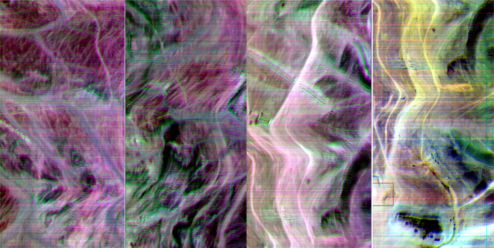
Figure 4.
The dataset “desert” is an hyperspectral image of a desert place taken by an airplane flying 10,000 feet above sea level. The resolution is 1.3 m/pixel, 286 × 2,640 pixels per waveband with 168 wavebands.

Figure 5.
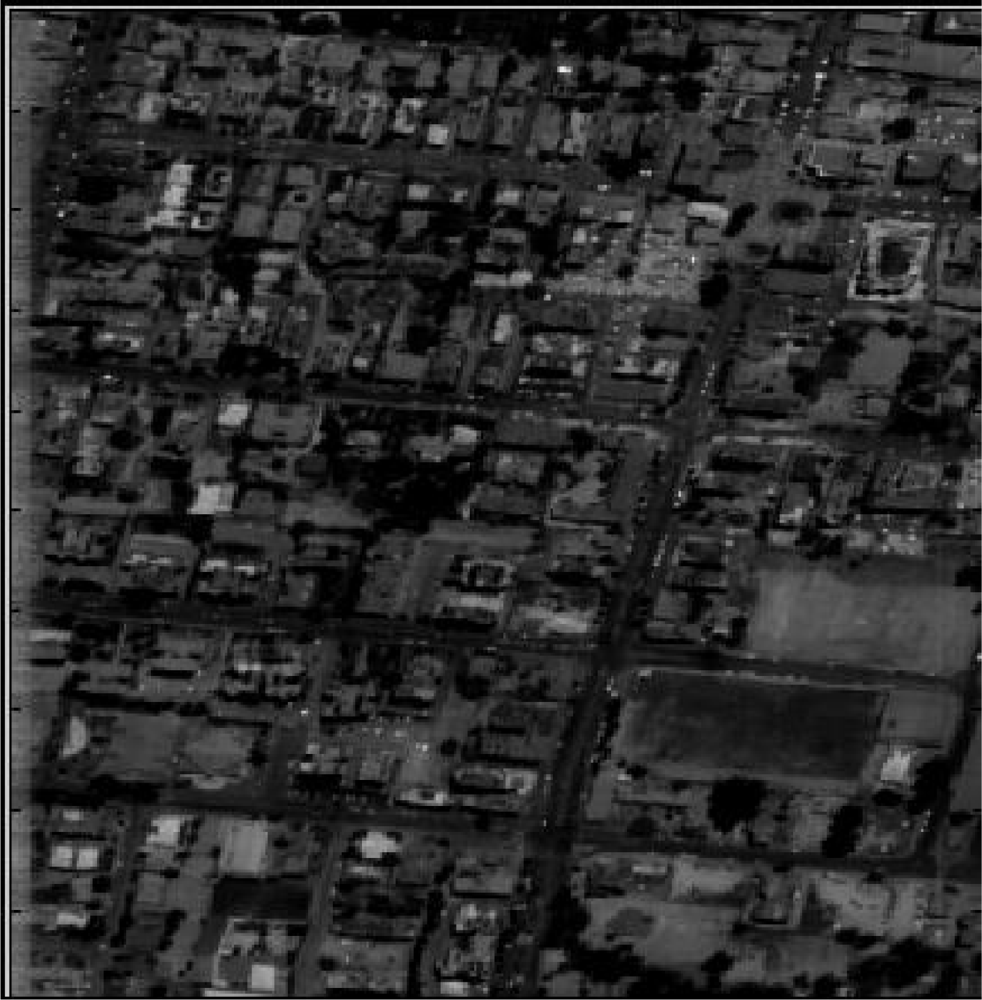
The dataset “city” is an hyperspectral image of a city taken by an airplane flying 10,000 feet above sea level. The resolution is 1.5 m/pixel, 294 × 501 pixels per waveband with 28 wavebands.
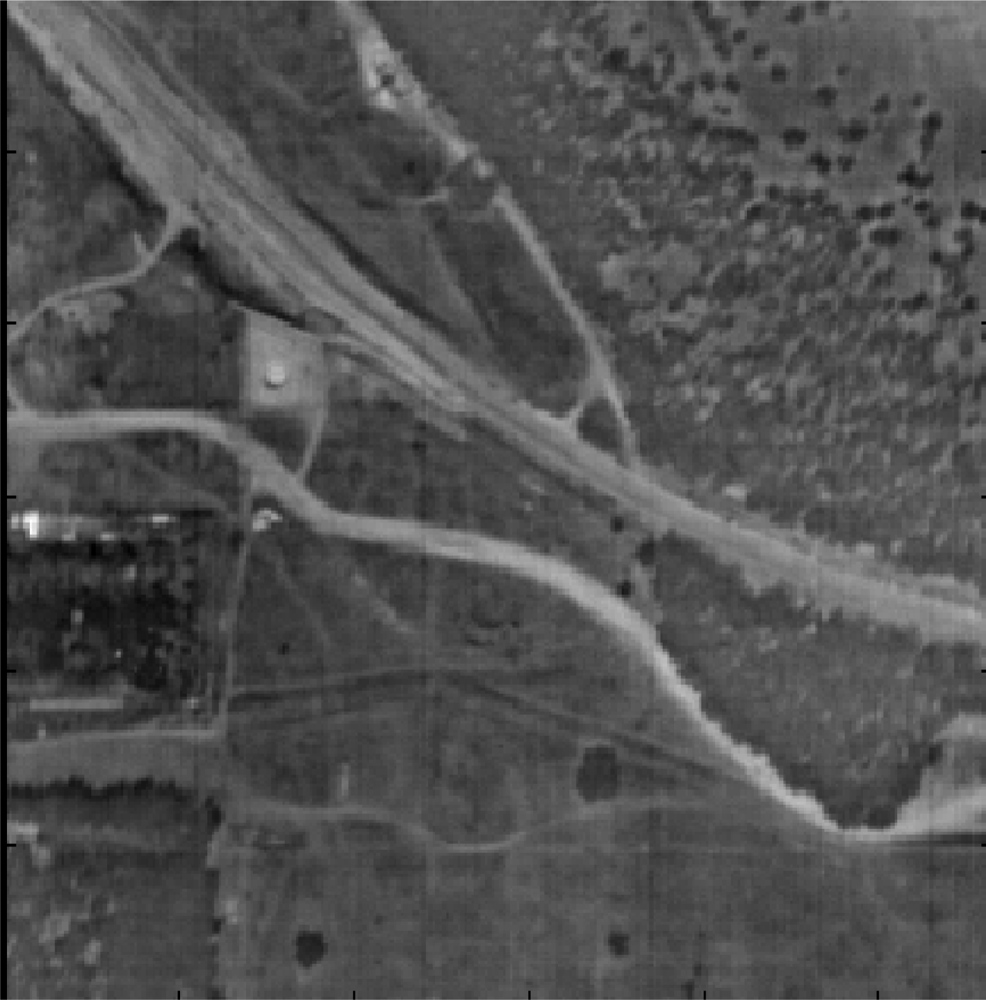
Figure 6.
The dataset “field” is an hyperspectral image of a field taken by an airplane flying 9,500 feet above sea level. The resolution is 1.2 m/pixel, 286 × 300 pixels per waveband with 50 wavebands.
3. Related Work
Up-to-date overview on hyperspectral unmixing is given in [4,5]. The challenges related to target detection, which is the main focus of this paper, are described in the survey papers [6,7]. They provide tutorial review on state-of-the-art target detection algorithms for HSI applications. The main obstacles in having effective detection algorithms are the inherent variability target and background spectra. Adaptive algorithms are effective to solve some of these problems. The solution provided in this paper meet some of the challenges mentioned in [6].
In the rest of this section, we divided the many existing algorithms into several groups. We wish to show some trends but do not attempt to cover the avalanche of related work on unmixing and target detection.
- Linear approach: Under the linear mixing model, where the number of endmembers and their spectral signatures are known, hyperspectral unmixing is a linear problem, which can be addressed, for example, by the ML setup [8] and by the constrained least squares approach [9]. These methods do not supply sufficiently accurate estimates and do not reflect the physical behavior. Distinction between different material’s spectra is conditioned generally by the distinction in the behavior of the first and second derivatives and not by a trend.
- Independent component analysis (ICA) is an unsupervised source separation process that finds a linear decomposition of the observed data yielding statistically independent components [10,11]. It has been applied successfully to blind source separation, to feature extraction and to unsupervised recognition such as in [12], where the endmember signatures are treated as sources and the mixing matrix is composed by the abundance fractions. Numerous works including [13] show that ICA cannot be used to unmix hyperspectral data.
- Geometric approach: Assume a linear mixing scenario where each observed spectral vector is given by r = x+n=Mγa+n, γa = s, where r is an L-vector (L is the number of bands), M = [m1, m2, . . . mp] is the mixing matrix (mi denotes the ith endmember signature and p is the number of endmembers present in the sensed area), s ≜ γa (γ is a scale factor that models illumination variability due to a surface topography), a = [a1, a2, . . . ap]T is the abundance vector that contains the fractions of each endmember ((·)T denotes a transposed vector) and n is the system’s additive noise. Owing to physical constraints, abundance fractions are nonnegative and satisfy the so-called positivity constraint . Each pixel can be viewed as a vector in a L-dimensional Euclidean space, where each channel is assigned to one axis. Since the set {a ∈ p : , ak > 0 for all k} is a simplex, then the set Sx ≜ {x ∈ L : x = Ma, , ak > 0 for all k} is also a simplex whose vertices correspond to endmembers.Several approaches [14,15,16] exploited this geometric feature of hyperspectral mixtures. The minimum volume transform (MVT) algorithm [16] determines the simplex of a minimal volume that contains the data. The method presented in [17] is also of MVT type, but by introducing the notion of bundles, it takes into account the endmember variability that is usually present in hyperspectral mixtures.The MVT type approaches are complex from computational point of view. Usually, these algorithms first find the convex hull defined by the observed data and then fit a minimum volume simplex to it. Aiming at a lower computational complexity, some algorithms such as the pixel purity index (PPI) [15] and the N-FINDR [18] still find the maximum volume simplex that contains the data cloud. They assume the presence of at least one pure pixel of each endmember in the data. This is a strong assumption that may not be true in general. In any case, these algorithms find the set of most of the pure pixels in the data.
- Extending subspace approach: A fast unmixing algorithm, termed vertex component analysis (VCA), is described in [19]. The algorithm is unsupervised and utilizes two facts: 1. The endmembers are the vertices of a simplex; 2. The affine transformation of a simplex is also a simplex. It works with projected and unprojected data. As PPI and N-FINDR algorithms, VCA also assumes the presence of pure pixels in the data. The algorithm iteratively projects data onto a direction orthogonal to the subspace spanned by the endmembers already detected. The new endmember’s signature corresponds to the extreme projection. The algorithm iterates until all the endmembers are exhausted. VCA performs much better than PPI and better than or comparable to N-FINDR. Yet, its computational complexity is between one and two orders of magnitude lower than N-FINDR.If the image is of size approximately 300 × 2, 000 pixels, then this method, which builds linear span in each step, is too computationally expensive. In addition, it relies on “pure” spectra which are not available all the time.
- Statistical methods: In the statistical framework, spectral unmixing is formulated as a statistical inference problem by adopting a Bayesian methodology where the inference engine is the posterior density of the random objects to be estimated as described for example in [20,21,22].
3.1. Linear Classification for Threshold Optimization
The description in this section, which is based on [23], is given since it is being used later in our development of the proposed methodology.
According to [23], a binary classification is frequently performed by using a real-valued function f : X ⊆ n → in the following way: the input x = (x1, ..., xn)T is assigned to a positive class if f(x) ≥ 0, otherwise, to a negative class. We consider the case where f(x) is a linear function of x with the parameters w and b such that
where (w, b) ∈ n × are the parameters that control the function. The decision rule is given by sgn(f(x)). w is assumed to be the weight vector and b is the threshold, then according to [23].
Definition 3.1 A training set is a collection of training examples (data)
where l is the number of examples, X ⊆ n and Y = {−1, 1} is the output domain.
The Rosenblatt’s Perceptron algorithm ([23,24], pages 12 and 8, respectively) creates an hyperplane ⟨w ·x⟩+b = 0 with respect to the training set S. It creates the best linear separation between positive and negative examples via minimization of measurement function of “margin” distribution λi = yi(⟨w, xi⟩ + b). The classification for (xi, yi) is correct when λi > 0.
The Perceptron algorithm is guaranteed to converge only if the training data are linearly separable. A procedure that does not suffer from this limitation is the Linear Discriminant Analysis (LDA) via Fisher’s discriminant functional [23]. The aim is to find the hyperplane (w, b) on which the projection of the data is maximally separated. The cost function (the Fisher’s function) to be optimized is:
where mi and σi are the mean and the standard deviation, respectively, of the function output values Pi = {⟨w · xj⟩ + b : yj = i} for the two classes Pi, i = 1, −1. From [23] we get the following definition.
Definition 3.2 The dataset S in Equation 4 is linearly separable if the hyperplane ⟨w · x⟩ + b = 0, which is obtained via the LDA algorithm ([23]), correctly classifies the training data. It means that λi = yi(⟨w, xi⟩ + b) > 0, i = 1, . . . , l. In this case, b is the separation threshold. If λi < 0, then the dataset is linearly inseparable.
Definition 3.3 The vector x ∈ n is isolated from the set P = {p1, ..., pk} ⊆ n if the training set S = ((x, 1), (p1, −1), ..., (pk, −1)) is linearly separable according to Definition 3.2. In this case, the absolute value of b is the separation threshold.
Suppose that we have a set S = {x1, .., xn} of n samples. First, we want to partition the data into exactly two disjoint subsets S1 and S−1. Each subset represents a cluster. The solution is based on the K-means algorithm ([25]). K-means maximizes the function J(e) (Equation (6)) where e is a partition. The value of J(e) depends on how the samples are grouped into clusters and on the number of clusters (see [25]).
where
is called “within-cluster scatter matrix” ([25]), l is the number of classes, Si are the classes and mi are the center of each class. SB is called “between-cluster scatter matrix” ([25]), where
, ni is the cardinality of the class i and m is the center for the dataset.
Definition 3.4 Let (w, b) be the best separation for the set S = {x1, ..., xn} ⊆ n via K-means and Fisher’s discriminant analyses [23,24]. (w, b) is called the Fisher’s separation and b the Fisher’s threshold for the data P.
When is a dataset separable? One criterion is when m1 −m−1 > max(diam(P1), diam(P−1)), where the notation in Equation (5) is used. Another criterion is:
Definition 3.5 ([25]) A dataset is separable if from Equation (6), J(e1) < J(e2) where e1 is the partition and the number of classes is 1 and e2 is the best partition into two classes. If J(e1) ≥ J(e2) then the dataset is inseparable and Fisher’s separation is incorrect.
4. Mathematical Preliminaries
This section describes the new mathematical background constructions that are needed for the proposed solution in this paper.
4.1. Definitions
Denote by prW (y) the orthogonal projection of the vector y ∈ n on the subspace W ⊂ n.
Definition 4.1 Given a vector x = (x1, x2, ..., xn). Denote modeɛ(x) ≜ argmaxp(card{i ∈ [1, .., n] : |p − xi| < ɛ}) where p is scalar. modeɛ(x) is called the mode with ɛ-error of the vector x.
Let q be a positive number. A vector x is called q − ɛ − sparse if the cardinality of its support {i : |xi| > ɛ} is less or equal to q.
The norm of the linear operator L, L : n → n, is ‖L‖ ≜ sup‖x‖=1 ‖Lx‖.
Definition 4.2 Let G be a vector space and assume that there is a finite subset ℑ ⊂ G. The set ℑ is ɛ-dense if for any element x ∈ G there is s ∈ ℑ such that ‖x − s‖ < ɛ.
Definition 4.3 Let G be a vector space and assume that the set ℑ is ɛ-dense in G. Let = {x ∈ G : ‖x − s‖ < r}. ℑ is homogeneous if for any s1, s2 ∈ ℑ and r > ɛ, holds. In this notation, is called the r − neighborhood of s.
For example, the integers set is ɛ-dense in the real numbers set when ɛ = 1. The set of rational numbers is ɛ-dense in for any ɛ. and are homogeneous.
Given two vector v1 and v2 in n. Assume that S1 and S2 are two linear operators in n and L is a linear span of {v1, v2}. We say that S1 and S2 are equivalent in relation to v1 and v2, denoted by S1 ∼ S2, if S1(L) = S2(L).
4.1.1. Sparse-Independency
Definition 4.4 Given two vectors y1 and y2 where their components are denoted by yj(i), j = 1, 2. Let S1 = {i : |y1(i)| > ɛ} and S2 = {i : |y2(i)| > ɛ}. If S1 ∩ S2 = ∅, then we say that y1 and y2 are ɛ − sparse − independent. If ɛ = 0 then they are called sparse − independent.
Let {e1, e2, ..., en} be a basis of n. Then, any subspace W = ei1⊕ei2 ⊕ ⋯ ⊕eik, where i1, i2, ..., ik is any subset of {1, 2, ..., n}, is called a basic subspace of n.
For example, in the 3D space with the standard basis {e1, e2, e3}, the plane, which is spanned by the vectors {e1, e2}, is a basic subspace. The plane, which is spanned by the vectors {(e1 + e3)/2, (e2 + e3)/2}, is not a basic subspace. The basic vectors {e1, e2, ..., en} of a basis subspace must be a subset of the standard basis n.
Given a pair of vectors y1 and y2 in n. Assume that L(y1, y2) is the linear span of y1 and y2. The basic subspace W ⊂ n is called a dependent basic subspace of y1 and y2 if dim(PrW L(y1, y2)) = 1.
Given a pair of vectors y1 and y2 in n. A natural number r is called a basis dependent rank of the vectors y1 and y2, if the two conditions hold:
- If W is a dependent basic subspace of y1 and y2 then dim(W) ≤ r;
- There exists a dependent basic subspace W of y1 and y2 where dim(W) = r.
For example, assume that y1 = (1, 2, 2, 3) and y2 = (2, 1, 1, −1) belong to 4 = e1 ⊕ ⋯ ⊕ e4. Let W = e2⊕e3. Then, z1 = PrW (y1) = (2, 2), z2 = PrW (y2) = (1, 1) and z1 = 2z2. Thus, we obtain that W is a dependent basic subspace for y1 and y2. It is clear that the dependency rank of the vectors y1 and y2 is 2.
If a pair of vectors y1 and y2 is sparse-independent, then their basis dependent rank is zero.
Assume that y ∈ n. The set Sɛ(y) = {i : |y(i)| > ɛ} is called the ɛ-support of y.
Given a pair of vectors y1 and y2 in n and ɛ > 0. Let r = min[card(Sɛ2 (y1)\(Sɛ(y1) ∩ Sɛ(y2)), card(Sɛ2 (y2)\(Sɛ(y1) ∩ Sɛ(y2))]. r is called the ɛ-sparse-independent-rank of the vectors y1 and y2.
Definition 4.5 Given a pair of vectors y1 and y2. Assume that r is their ɛ-sparse-independent-rank and b is a basis dependent rank of the vectors y1 and y2. These two vectors are called a ɛ-sparse-ergodic independent if r > b.
- For example, sparse-independent vectors have a basis dependent rank zero and they are ɛ-sparse-ergodic independent.
- Denote by PrW (y) the orthogonal projection of the vector y ∈ n onto the subspace W ⊂ n.
- Let q be a positive value. A vector x is called q − ɛ − sparse if the cardinality of its support {i : |xi| > ɛ} is less or equal to q.
4.1.2. Classification
Assume that Γ is a set of vectors from n that has zero average and a singular norm. Γ is called the set of weak classifiers. Assume that Φ and Ω are two subsets in n. The vector ξ ∈ Γ is called a optimal weak classifier for Φ and Ω relative to Γ if for any vector a ∈ Φ and b ∈ Ω, ξ = argmaxζ∈Γ ⟨a, ζ⟩ holds and ⟨ξ, b⟩ = 0.
Our goal is to separate between the sets Φ and Ω. The distinction between these two sets can be described in different ways. Behavior of the first or second derivatives of the vectors can be one way. Another way can be the characteristics of the sets such as the relation between the maximum and the minimum in the vectors. These properties define a set of weak classifiers Γ.
Next, we introduce two families of sensors.
The set Γ ⊆ n is called a d − support local − characteristic set of weak classifiers (d ≪ n) if for any ξ ∈ Γ, diam{i :| ξi |> 0} ≤ d holds.
Given ɛ > 0. The set Γ ⊆ n is called a d − support global − characteristic set of weak classifiers if for any ξ ∈ Γ, card{i :| ξi |> 0} = d holds and {i :| ξi |> 0} is an ∊ − dense (Definition 4.2) in the set {1, 2, ..., n}.
Definition 4.6 Assume that {ξ1, ξ2, ..., ξm} are the optimal weak classifiers for two sets Φ and Ω. Define a linear operator Ξ : n → m such that Ξ(a) = (⟨a, ξ1⟩, ⟨a, ξ2⟩, ..., ⟨a, ξm⟩). This linear operator is called the separator projection.
Proposition 4.1 Assume T is the target’s spectrum, B and P are the spectra of the background and the mixed pixel, respectively. Parameter t obeys the linear mixing model P = tT + (1 − t)B. Let Φ = {T} and B ∈ Ω, where Ω is a set of background vectors. Assume that {ξ1, ξ2, ..., ξm} are optimal weak classifiers for two sets Φ and Ω. Ξ = [ξ1, ξ2, ..., ξm] is a projection separator and T1 = Ξ (T), P1 = Ξ(P), B1 = Ξ (B). Then, ‖P1‖ = t‖T1‖ and corr(P1, T1) = 1.
Proof: P1 = Ξ(tT + (1 − t)B) = tΞ(T) + (1 − t) Ξ(B). Since Ω ⊂ ker(Ξ) and B ∈ Ω, then (1 − t) Ξ(B) = 0 and P1 = tΞ(T) = tT1.
4.2. The Main Propositions
The goal of this section is to generate the conditions for which the vectors provide a solution for the unmixing problem given by Equation (2).
Lemma 4.1 Let B be an unknown background spectrum, T and P are the known spectra of the target and of the mixed pixel, respectively. The parameter t satisfies the linear mixing model P = tT +(1−t)B. If for any fixed positive value γ > 0, 0 < ɛ < 1 , S1 = {i : |B(i)| > γ} and S2 = {i : |T (i)| >γ/ɛ} we have that card(S2 \ S1) ≥ card(S1 ∩ S2), then t = modeɛζ(Definition 4.1) where ζ is a vector whose coordinates are and T1 = {T |‖T ‖ >γ/ɛ}.
Proof: Let
and let
, then ξ = t + (1 − t) ζ. Let W = (S2\S1) and V = (S2 ∩ S1), then |W| ≥ |V|, W ∩ V = ∅, {ζ(i)}i∈W ∩{ζ(i)}i∈V = ∅ and {ζ(i)} ={ζ(i)}i∈W ∪ {ζ(i)}i∈V. If i ∈ W then |ζ(i)| =
< γ/(γ/ɛ) = ɛ and card({i : |ζ(i)| ≥ ɛ}) ≤ |V| ≤ |W|. Thus, modeɛ(ζ) = 0 and modeɛ(ξ) = t.
¿From Lemma 4.1 we get Proposition 4.2.
Proposition 4.2 Let B be an unknown background spectrum and T and P be the known spectra of the target and of the mixed pixel, respectively. The parameter t satisfies the linear mixing model P = tT + (1 − t)B. Let T1 = {T |‖T ‖ > γ} and ξ is a vector with the coordinates. Assume that B and P are ɛ − sparce − independent. Then, modeɛ/γ (ξ) = t.
Proposition 4.3 Assume that B is the unknown background spectrum where T and P are the known spectra of the target and of the mixed pixel, respectively. Assume that the parameter t satisfies the linear mixing model P = tT + (1 − t)B. If B and T are orthogonal, then t = ⟨T, P ⟩/‖T ‖2.
Proof: ⟨T, P ⟩ = ⟨T, t · T + (1 − t)B⟩ = t · ⟨T, T ⟩ = t · ‖T ‖2.
Note that if ⟨T, B⟩ = ∊, then the variance of this estimation error is ∊ /‖T‖2. “Sparse-independency” and orthogonality are strong conditions. Theorem 4.1 shows that “ɛ-sparse-ergodic independency” also provides a solution for the linear unmixing problem.
Theorem 4.1 Given ɛ > 0, B is an unknown background spectrum, T and P are the known spectra of the target and of the mixed pixel, respectively. The parameter t satisfies the linear mixing model P = tT + (1 − t)B. Assume B and P are ɛ-sparse-ergodic independent (see Definition 4.5). Ti denotes the ith coordinate of the vector T. Let T1 = {Ti : |Ti| > ɛ} and ξ is a vector with the coordinates. Then, modeɛ(ξ) = t.
Proof: Let
and
. ξ = t + (1 − t)ζ , then we only need to prove that modeɛ(ζ) = 0. Assume that p ≠ 0 is a real number. Let Ω = {i|Bi = pTi} and Λ = {i|Bi < ɛ2 ∧ Ti > ɛ}. The ɛ-sparse-ergodic independency (see Definition 4.5) of B and T follows from the fact that card(Ω) < card(Λ), because if W = ⊕i∈Ω ei, then W is a dependent basic subspace of T and B and dim(W) = card(Ω). Note that {i|Bi < ɛ2 ∧ Ti > ɛ} = {i|ζi < ɛ} and {i|Bi = pTi} = {i|ζi = p}. From the condition card({i|ζi = p}) < card({i|ζi < ɛ}) follows that modeɛ(ζ) = 0.
Now we show how to obtain the “ɛ-sparse-ergodic independency” (see Definition 4.5).
Theorem 4.2 Assume that {v1, v2} ⊂ n, ⟨v1, v2⟩ = 0, ɛ > 0. Let Λ = {S1, S2, ..., Sr} be the ɛ-dense and homogeneous set of isometrics operators in n. Then,
w1 ≜ [v1, S1(v1), S2(v1), ..., Sr(v1)] and w2 ≜ [v2, S1(v2), S2(v2), ..., Sr(v2)] are ɛ-sparse-ergodic independent.
The rest of this section proves Theorem 4.2.
Proposition 4.4 For any pair of orthogonal vectors {v1, v2} ⊂ 2 such that ⟨v1, v2⟩ = 0, for any linear operator S : 2 → 1 where ‖S‖ = 1 and for any real t ≠ 0, the inequality P [S(v2) = t · S(v1)] < P [S(v2) = 0] holds when P is probability.
Proof: Any linear operator S : 2 → 1 with ‖S‖ = 1 can be represented as S(x) = ⟨s, x⟩ where s = (s1, s2) is a vector with ‖s‖ = 1.
Consider
to be a rotation of 2. This rotation splits the linear operator S into a product of the rotation operator with the orthogonal projection such that S = Ŝ ○ Pr1 where Pr1(x1, x2) ≜ (x1, 0).
We can choose the basis {e1, e2} of 2 such that v2 = (a, 0) and v1 = (0, b). In this representation,
. For any t ∈ , the solution of t = (−a/b) tan(φ) exists.
In addition,
has a minimum in zero. Hence, the size of the set {φ : | tan(φ)| < ɛ} is more than the size of the set {φ : | tan(φ) − t| < ɛ} for t ≠ 0.
Corollary 4.1 Let {S1, S2..., Sr} be ɛ-dense and homogeneous set (Definitions 4.2 and 4.3) of the linear operators 2 → 1 and {v1, v2} is orthogonal in 2. Then, the vector ς with the coordinates, i = 1, …, r, has modeɛ(ς) = 0.
Proposition 4.5 Given a pair of orthogonal vectors {v1, v2} ⊂ n, ⟨v1, v2⟩ = 0 and ɛ > 0. Assume that S1, S2, ..., Sr is an ɛ-dense and homogeneous set of isometrics operators in n. Then, the vector ς, which has the coordinates, i = 1, . . . , n, α = 1, . . . , r, has modeɛ(ςi,α) = 0 where is the ith coordinate of the vector.
Proof: Denote Λ = {S1, S2, ..., Sr}. The set of χ coordinates is divided into the union of the subsets τi where τi = {ςi,α}Sα∈Λ α = 1, . . . , r. We have to show that modeɛ(τi) = 0, i = 1, . . . , n. Assume that θi is a projection to coordinate i, such that for x = (x1, ..., xn), θix = xi. Assume that L is a linear span of {v1, v2}. Define Rα = θi ○ Sα where Rα: 2 → 1. Our assumption was that Λ = {S1, S2, ..., Sr} is ɛ-dense and homogeneous. Therefore, {R1, R2, ..., Rr} is ɛ-dense and homogeneous too. Then, Corollary 4.1 implies modeɛ(τi) = 0.
Proof: proof of Theorem 4.2: Let L be the linear span of w1 and w2 from nr = ⊕S⊂Λ n. If the theorem is not true, then there is basic subspace W in ⊕S⊂Λ n such that dim(W) = q and dim(Prw(L)) = 1. It means that w1|W = s and w2|W = t · s, t ≠ 0, such that dim(W) > card{i|(w2)(i) = 0 and (w1)(i) ≠ 0}. This means that a vector with the coordinates
, i =1, . . . , nr, has modeɛ(ςi) = t ≠ 0. This contradicts Proposition 4.5.
5. Random Orthogonal Transformation Algorithm for Unmixing (ROTU)
We denote the first derivative of a spectrum of a pixel X by d(X) and it is called the d − spectrum of the pixel X.
For independent spectra and for special type of dependent spectra, which will be defined below, we can use a faster and less computationally expensive method than [2] (Section 4). This is described in this section. This method works well if the d − spectra of different materials are related by the so-called sparse − independent (see Definition 4.4). This relation will be described below. If they are not sparse − independent then this method may generate false alarms.
We assume now that the conditions in Section 2 hold. We are given the target’s spectrum T and the mixed pixel spectrum P. Their relationship is described by Equation (2) via the average background spectrum B, which is a mix of the background spectra without the presence of the target, such that
and
Our goal is to estimate t, denoted by t̂, which will satisfy Equation (7) provided that B and T have some independent features. Once t̂ is found, the estimation of an unknown average background spectrum B, denoted by B̂, can be calculated by B̂ = (P − t̂T)/(1 − t̂).
5.1. The Unmixing Algorithm
Generally speaking, spectra of different materials have different sections in them: some sections are mutually correlated, some sections are smooth and some have sections with oscillatory behavior. Large first and second derivatives are used as characteristic features for a spectral classification.
Some section in the spectrum can be autocorrelated. Let D = (D1, D2) be a pair of the first and the second derivatives operator. Our assumptions imply that D(T) and D(B) are more independent than T and B. The D operator reduces the correlation between spectra and makes them more independent.
Let x be a spectrum. We denote by a d − spectrum the vector Dx. If two d − spectra of different materials are statistically independent (or orthogonal), then estimating t can be obtained by using Proposition 4.3. Statistical independency is a strong condition. Sometimes we have sparse − independency for the d − spectra. The sparse-independency condition yields its estimation from Proposition 4.2. In general, we have ɛ deviation from orthogonality and the condition of sparse − independency never holds.
The unmixing algorithm has the following steps:
Step 1: The operator D is applied to T and P. We assume that |corr(DT, DB)| < ɛ.
Step 2: Assume that Λ = {S1, S2, ..., Sr} is random isometric rotations in n, W : n ↣ 2nr = ⊕S⊂Λ n is the embedding of n into 2rn such that
Step 3: Construct the vector ς with the coordinates
Step 4: Estimation of t, denoted by t̂, is computed by
, i = 1, …, 2rn. B is estimated by B̂ = (P − t̂T)/(1 − t̂).
The vectors wT , wB and wP are related by wP = t · wT + (1 − t) · wB, where wB is unknown. Proposition 4.5 and Theorems 4.1 and 4.2 yield that {wT, wB} are ɛ-sparse-ergodic independent (Definition 4.5) and the modeɛ(ς) of the vector ς, which have the coordinates
is modeɛ(ς) = 0.
It follows that
estimates t. As the number of operators is increased then this estimate becomes more accurate.
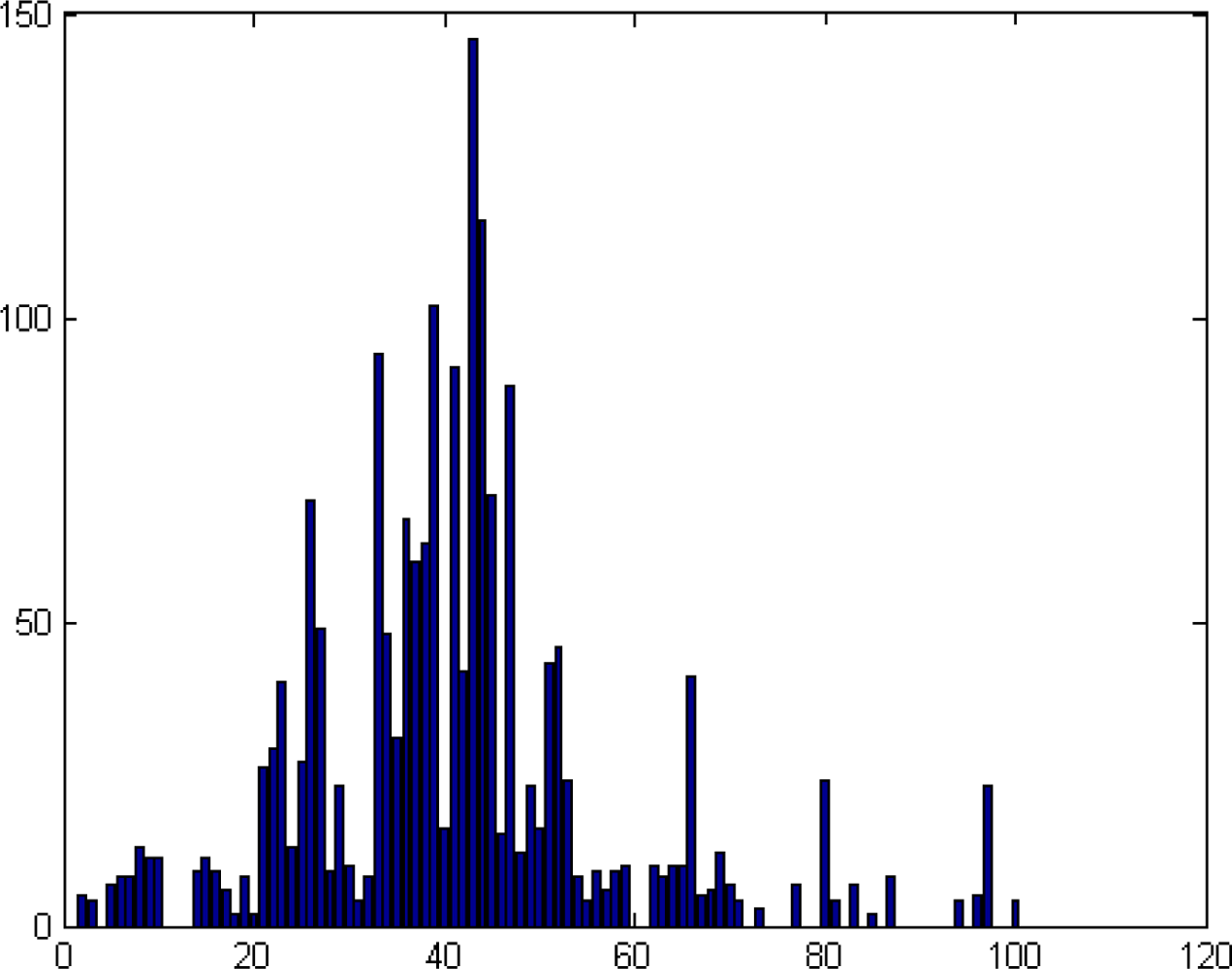
Definition 5.1 Equations (8–11) denote the vector ζ = (ζk) with the set of coordinates, k = 1, . . . , 2rn. Assume ɛ > 0 and b = {0, ɛ, 2ɛ, 3ɛ, 4ɛ, . . . , 1 = mɛ} is a partition of [0, 1]. Then, the vector H such that Hi = card{k|iɛ − ɛ/2 < ζk ≤ iɛ + ɛ/2}, i = 1, . . . , m, is an histogram of ζk related to the partition b. This histogram is called the “unmixing histogram”.

Figure 7.
The “unmixing histogram” for Figure 3. The x-axis is the b partition of [0, 1], ɛ = 0.01. The y-axis is the number of coordinates that belongs to each interval in the b partition
In Figure 7, we can see the distribution of the values of the vector ζ on the interval [0, 1], where the partition step is 0.01. This histogram shows that the mode of this distribution is 0.4 = 40 · 0.01. Thus, t is estimated by t̂ = modeɛ(ξ) = 0.4, where the vector ξ is computed by Equation (11). As long as t̂ is known, we can estimate the spectrum of the background B̂ = (P − t̂T)/(1 − t̂). The comparison between B and B̂ is shown in Figure 8.

Figure 8.
The solid line corresponds to the real spectrum of the background and the dotted line corresponds to the estimated spectrum of the background
5.2. Experimental Results
1. Experiment with random spectral signatures. Assume the vectors B and T were randomly generated. B is unknown. The vector P was computed by P = tT + (1 − t)B for t = 0.1, 0.3, 0.7, 0.9. Figure 9 displays the plots of P , T and B for t = 0.7. The vector P corresponds to the spectrum of the mixed pixel, T corresponds to the known target spectrum and B corresponds to an unknown background spectrum.
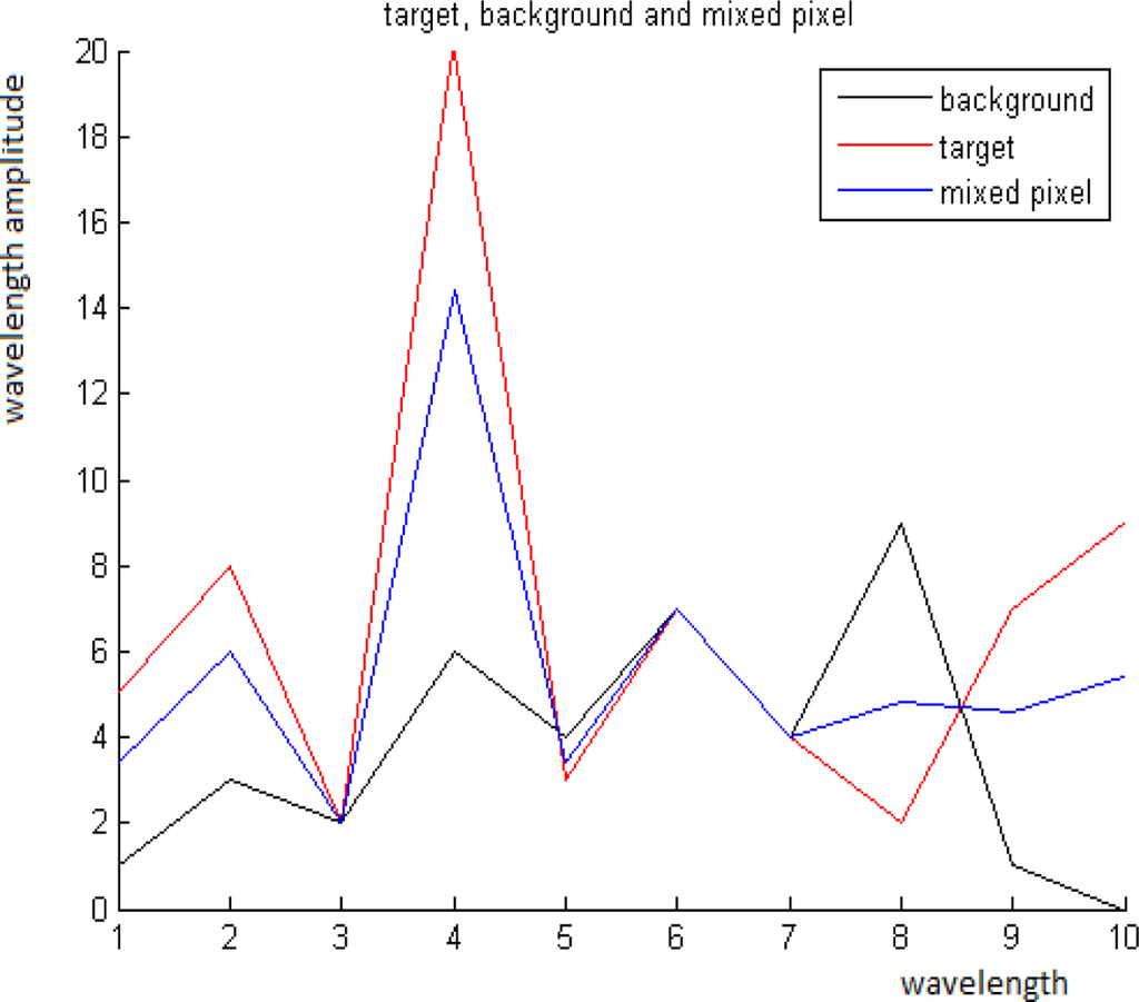
Figure 9.
Random spectral vector signatures.
The ROTU algorithm, which estimates t, is applied to the pair P and T with different t values. Then, the estimations of t̂and t are compared. Once t̂ is obtained then the unknown B is estimated by B̂ = (P − t̂T)/(1 − t̂).
The “unmixing histogram” from Definition 5.1 is displayed in Figure 10 for several t values.
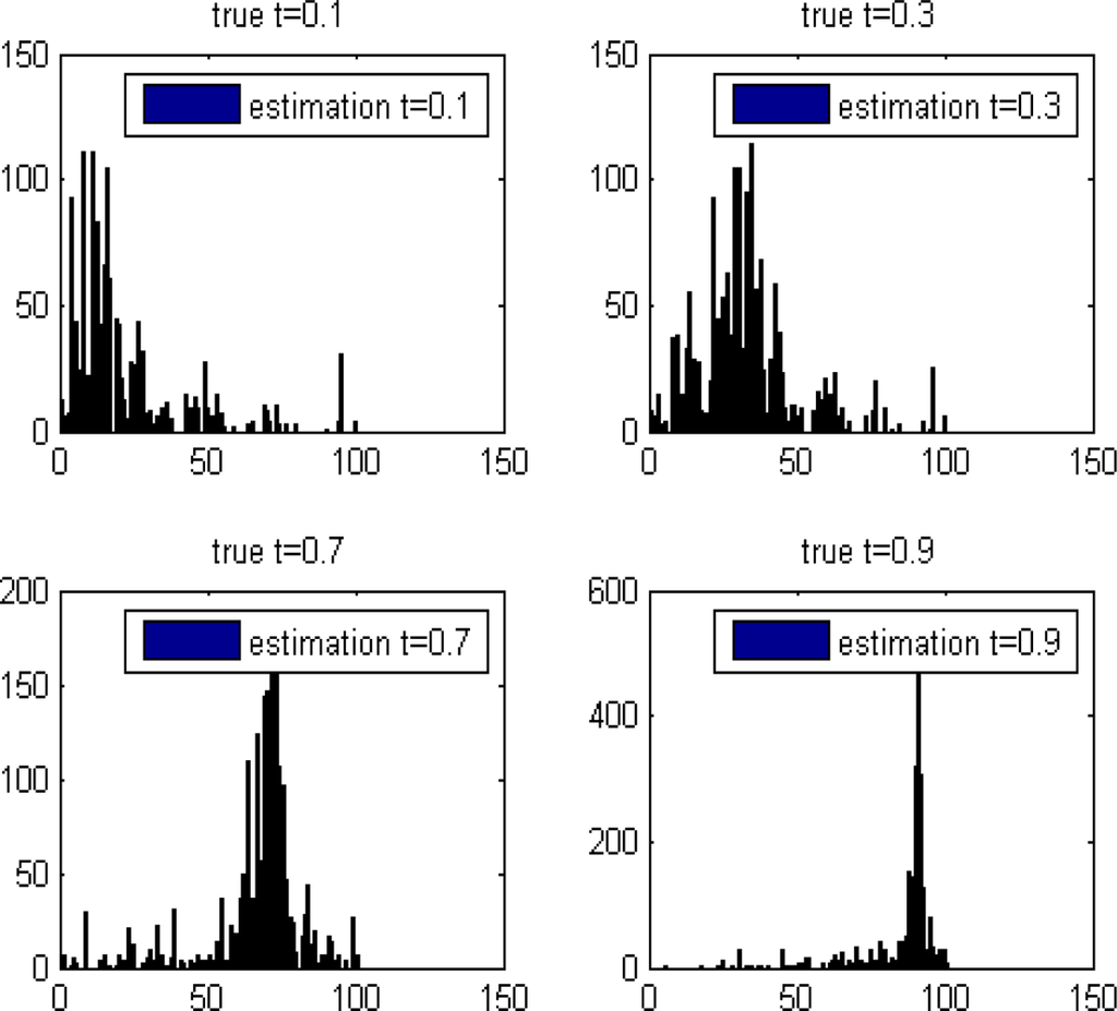
Figure 10.
The “unmixing histogram” from Definition 5.1 for different t values. The horizontal and the vertical axes are the b partition of [0, 1], ɛ = 0.01. The cardinality of the coordinate’s set belongs to each interval in the b partition. The boxes inside the graphs is the estimated results from the application of the ROTU algorithm.
t = 0.3 vs. t̂ = 0.3, t = 0.7 vs. t̂ = 0.7, t = 0.9 vs. t̂ = 0.9 and t = 0.1 vs. t̂ = 0.1. In all these cases, t̂ = t. It means that the reliability of our algorithm on these datasets is 100%.
2. Experiment with Spectra of Real Materials. The spectra B and T of two materials were taken from a database of signatures. They are presented in Figure 11. P is computed by P = tT + (1 − t)B for t = 0.3, 0.55, 0.7, 0.8.

Figure 11.
The spectra T and B of different materials from the database of signatures, where the x- and y-axes are the wavebands and their values, respectively
P and T are known while B is unknown. The ROTU algorithm is applied to the pair P and T for t = 0.3, 0.55, 0.7, 0.8. The ROTU algorithm estimates t by t̂. Once t̂ is obtained, then the unknown B can be estimated from B̂ = (P − t̂T)/(1 − t̂).
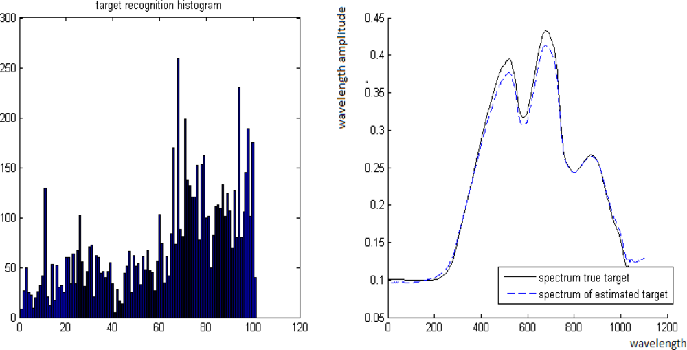
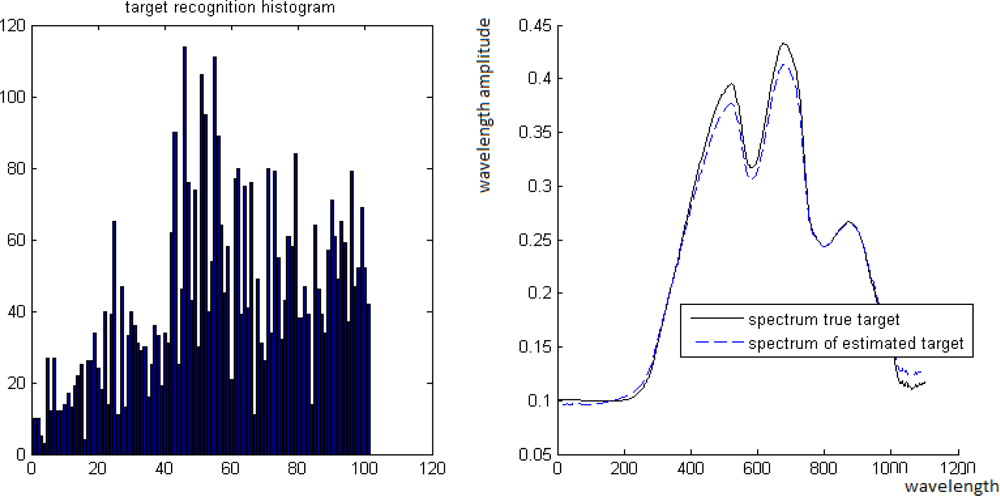
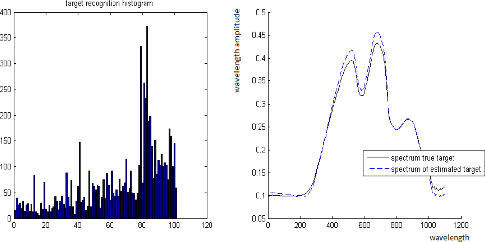
The “unmixing histograms” from Definition 5.1 and the comparison between B and its estimate B̂ are given below. In each of the Figures 12–15, the horizontal axes of the left images represent the b partition of [0, 1], ɛ = 0.01. The vertical axes of the left images represent the cardinality of the coordinate’s set that belongs to each interval in the b partition.
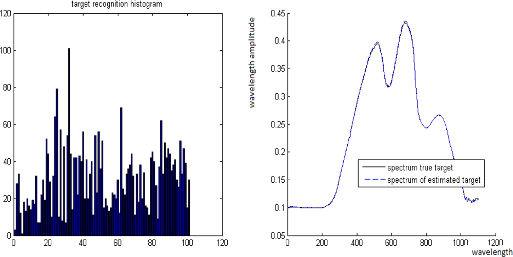
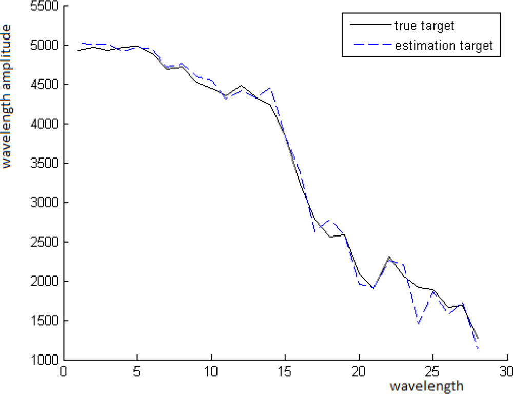
Figure 12.
Left: The “unmixing histogram” from Definition 5.1. Right: Comparison between T and its estimate T̂.

Figure 15.
Left: The “unmixing histogram” from Definition 5.1. Right: Comparison between B and its estimation B̂
Case 1. True value is t = 0.3 where its estimate is t̂= 0.28.
Case 2. True value is t = 0.7 where its estimate is t̂= 0.69.
Case 3. True value is t = 0.49 where its estimate is t̂= 0.45.
Case 4. True value is t = 0.8 where its estimate is t̂= 0.82.
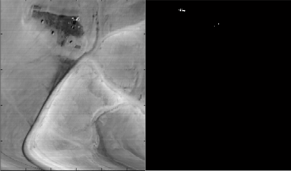
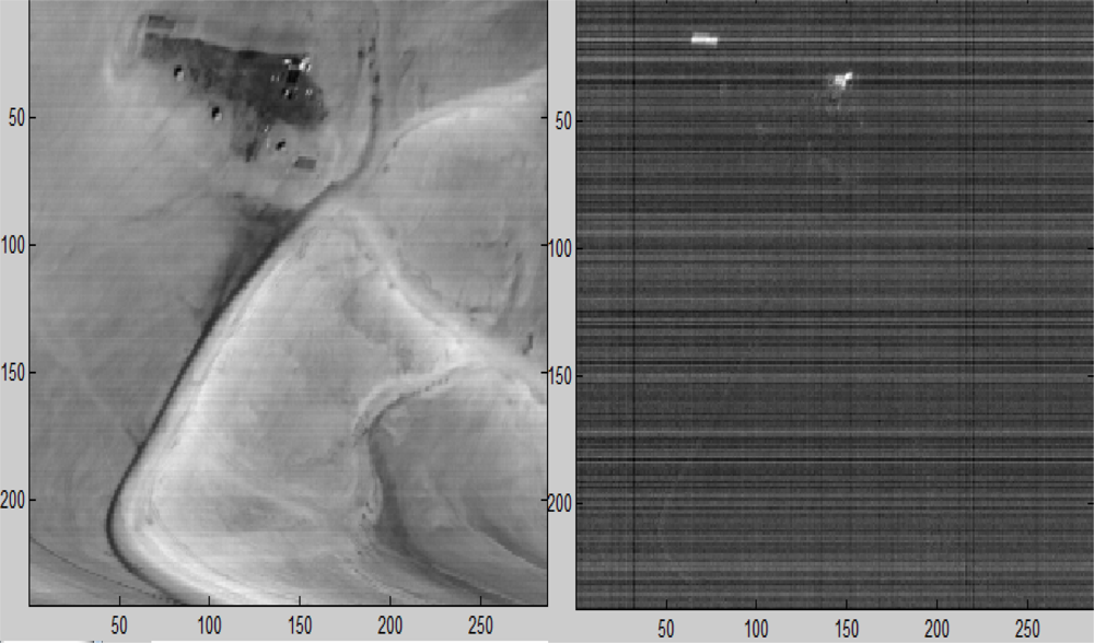
3. Experiment with sub- and above-pixel’s target recognition. We present the results from the application of the ROTU algorithm to two different types of scenes: (1). “Desert” (see Figure 4) has targets that occupy more than a pixel. It is shown in Figure 16. “Field” (see Figure 6) has a subpixel target. It is shown in Figure 17. In each figure, the parameter t, which was introduced in Equation (7), means the portion of the target’s material in the detected pixel (fractional abundance).

Figure 16.
Left: The scene from Figure 4. Right: Points that contain a target in above pixel when t = 1.
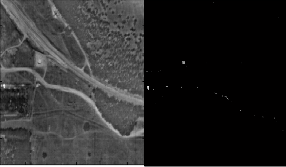
Figure 17.
Left: The scene from Figure 5. Right: Points that contain a target in a sub-pixel when t > 0.5.
6. Classification for an Unmixing (CLUN) Algorithm
In this section, we present another unmixing algorithm that is based on classification. This method works fast and does not require any conditions on the relation between the background and the target spectra. The spectra of the target and the background can be correlated and their derivatives can be correlated too. We outline the following consecutive steps in a target identification via classification by HSI learning:
- Learning phase: Finding typical background features by the application of PCA to the spectra of randomly selected multi-pixels from the scene where a multi-pixel is one pixel with all its wavelengths;
- Separation of the target’s spectra from the background via a linear operator, which is obtained from the “learning” phase;
- Construct a set of sensors which are highly sensitive to targets and insensitive to background;
- Embedding the spectra from the scene into a space generated by “good” sensors vectors and detect the points that contain the target that has a big norm value.
6.1. Sensor Building Algorithm (SBA)
Let V = {v1, ..., vs} be a set of multi-pixels spectra that were randomly chosen. We assume that the majority of the pixels from the scene are background pixels. Hence, after the application of PCA to V we get information about the background and not about the targets. Assume that Ω = {w1, ..., wp} are the principal components of the PCA of V and Φ is a set of the known targets spectra. In our approach, Φ = {T} has only one vector, which is the vector of the target’s signature. Our goal is to separate between the two sets Ω and Φ via the sensor building algorithm (SBA) that is discussed next. Algorithm 1: Outline of SBA
- Let T be the target’s spectrum: Construct the functionsuch that ξ maximizes F (ξ) and W is a weight coefficient.
- Given a set of weak classifiers Γ: Perform s iterations to collect the s functions from Γ each of which provides a local supremum for the function F. Each function ξ from Γ is named a “weak classifier”. If s is big (for example, s = 1000), then our algorithm becomes more accurate while the computational time becomes longer.
- Construct the “strong classifier”: It is a linear operator Ξ = [ξ1, ξ2, ..., ξs], where each ξi was obtained in step 2. This operator is a “projection separator” (see Proposition 4.1).
- Construct T1 = Ξ (T) (see Definition 4.6), where T is the spectrum of the target.
Detailed description of the “weak classifier” collection:
- Choose an integer r > 1000 and a value for ∊ > 0.
- First iteration: Select a subset Γ̂ of r vectors from Γ via random choices.
- Assume s−1 iterations took place. We describe now the sth step. We select a subset Γ̂ of r vectors from Γ via a random choice such that for each ξi, i = 1, .., s − 1, dist(Γ̂, ξi) > ∊ holds.
- Let ξs = argmax{F (ξ)|ξ ∈ Γ̂}.
Assume P is the current pixel’s spectrum. Proposition 4.1 contains the following two properties where Ξ is defined in Definition 4.6.
- corr(Ξ(P), T1) is close to 1.
- t = ‖Ξ(P)‖/‖T1‖ is the portion of the target in the current pixel.
6.2. Description of the CLUN Algorithm
We assume that we have the same conditions as in Section 2. We are given the target’s spectrum T and the mixed pixel spectrum P . Their relationship is described by Equation (2) using the background’s average spectrum B, which is the mix of the background’s spectra without the presence of the target, such that
and
Our goal is to estimate t, denoted by t̂, which will satisfy Equation (14) provided that B and T have some independent features. Once t̂ is found, the estimation of an unknown background average spectrum B, denoted by B̂, is computed by B̂ = (P − t̂T)/(1 − t̂).
The CLUN algorithm contains the following steps:
- Apply the sensor building algorithm (SBA - Algorithm 1).
- Construct an operator that is the projection separator Ξ(P) from Definition 4.6.
- Apply the operator Ξ(P) to each pixel’s spectrum.
Let {P1, . . . , Pω} be the spectra dataset from all the pixels in the scene. Denote Yi = ‖Ξ (Xi)‖. There are two possibilities for the dataset {Y1, . . . , Yω} ⊆ +:
- The set {Y1, . . . , Yω} is separable according to Definition 3.5;
- The set {Y1, . . . , Yω} is inseparable according to Definition 3.5.
From Definition 3.5, a dataset is separable if J(e1) < J(e2) where e1 is the partition and the number of classes is 1 and e2 is the best partition for the two classes. The function J(e) measures the separation quality between the clusters. If J(e1) ≥ J(e2), then the dataset is inseparable and Fisher’s separation is incorrect.
In the first case, (w, b) is the best separation between two clusters of the set S = {Y1, . . . , Yω} ⊆ + according to Definition 3.4 and b is the Fisher’s threshold for this separation. Then, {i|Yi > b} is the set of pixels that contains the targets. In the other case, there are no pixels that contain the targets.
Assume Pi is the spectrum of the current pixel. Assume ‖Ξ(Xi)‖ > b. Then, according to our assumption Pi contains the target’s spectrum as a linear component. It means that i is a suspicious pixel. corr(Ξ(P), T1) is close to 1, then t = ‖Ξ(P)‖/‖T1‖ is the portion that contains T in the current pixel.
6.3. Implementations of the CLUN Algorithm
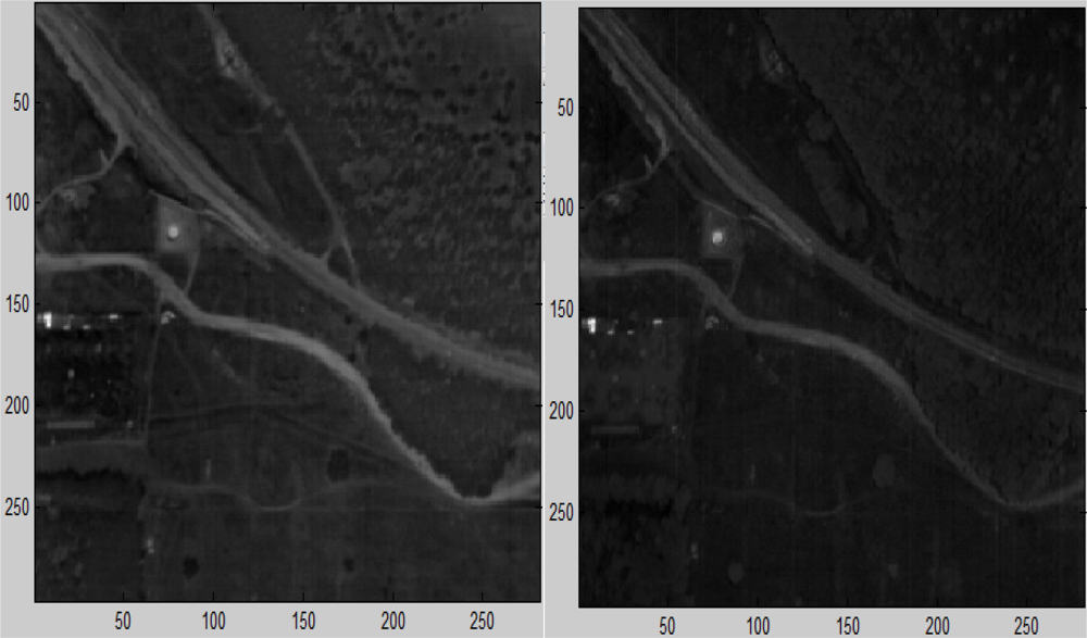
We present the results from the application of the CLUN algorithm to hyperspectral images where the target once occupies more than a pixel and once it occupies a subpixel. In Figures 18 and 19, the parameter t, which was introduced in Equation (7), is the portion of the target in the current pixel.

Figure 18.
Left: The source image. Right: The result from the application of the projection separators. The white points contain targets with t ≥ 0.7.

Figure 19.
Left: The source image. Right: The result from the application of the projection separators. The white points contain a targets with t ≥ 0.7.
To separate between Ω and Φ, we utilize the following sets types Γ:
- d − support local − characteristic is the set of weak classifiers.
- d − support global − characteristic is the set of weak classifiers.
- Assume that Γ = {ξi,j} is the set of weak classifiers where ⟨ξi,j, X⟩ = Xi − Xj. This set of weak classifiers works well if the vectors from Φ and Ω have a low entropy. It means that many coordinates have equal values and random differences between some coordinates provide sparse and independent behavior.
Figures 20 and 21 illustrate the separation between Ω and Φ. In this example, we used the d−support local − characteristic as the set of weak classifiers to achieve this separation.
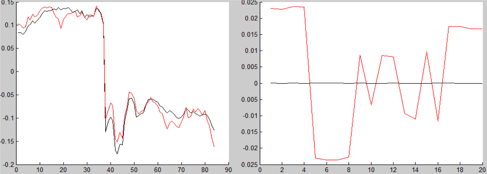
Figure 20.
Left: The red line is the target’s spectrum and the black line measures the background (it was taken from the scene in Figure 4). Right: The same two vectors after the projection of the separating mapping. The x-axis represents the wavelengths and the y-axis represents the wavelengths amplitude before (left) and after (right) the application of the projection.
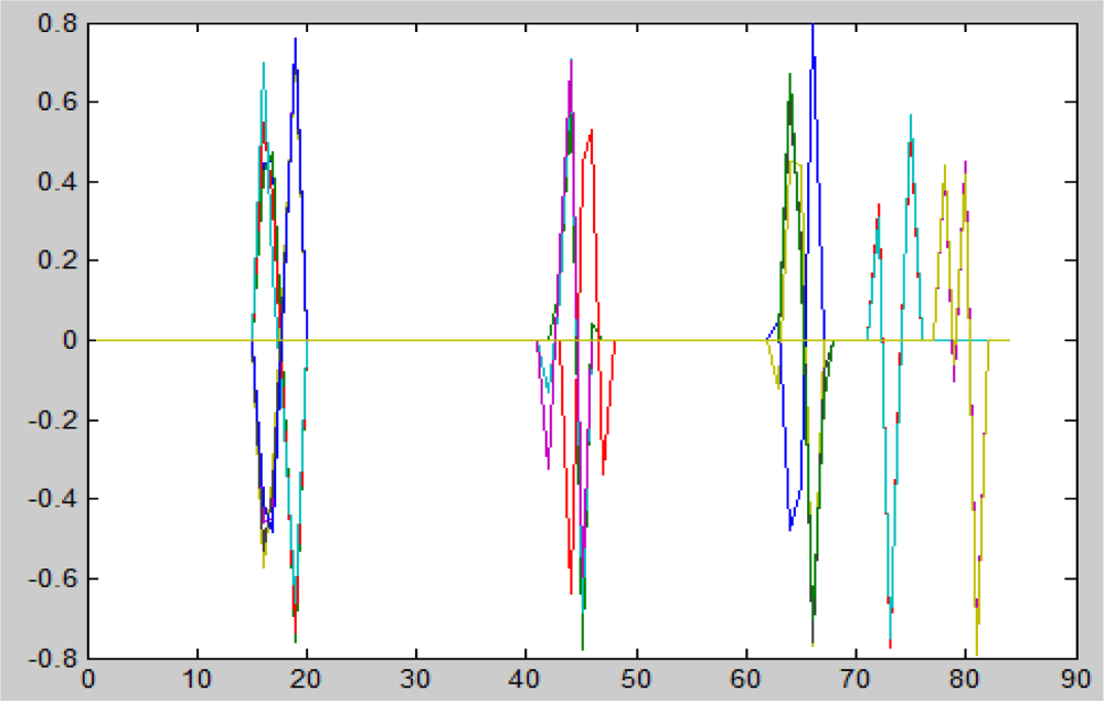
Figure 21.
Representation of 20 sensors (“weak classifiers”) with small supports. They were obtained as shown in Section 6.1. The x-axis represents the wavelengths index and the y-axis represents the values of the sensor-function.
Figure 22 illustrates the other type of situation. The spectrum was taken from the scene “City” (Figure 5). Here the features, which are located in small segments, have noise. Hence, global features sensors are required to separate between the target’s spectrum and the background’s spectrum.
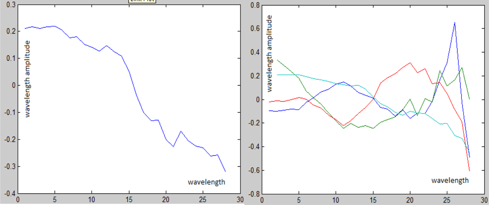
Figure 22.
Left: The target’s spectrum. Right: The principal components of the background’s spectra. The spectra was taken from the “city” image (Figure 5).
Figure 23 shows how the wavelengths after the projection by the application of PCA.
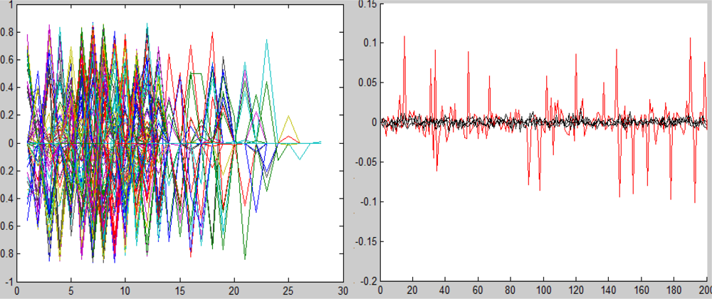
Figure 23.
Left: This plot represents 200 d-support global-characteristic sensors, d = 4. They were obtained as shown in Section 6.1. Right: The spectrum of the target (red) and the PCA of the background (black) after the application of the projection separators. The x-axis represents the wavelengths and the y-axis represents the wavelengths amplitude before (left) and after (right) the application of the projection.
6.4. Experimental Results for Sub- and Above Pixel Target Recognition
We present the results from the application of the CLUN algorithm to three different types of scenes (Figures 4–6). In the first scene (Figure 18), the target occupies more than a pixel. The other two scenes (Figures 19 and 24) contain subpixel targets. In each figure, the parameter t, which was introduced in Equation (7), is the portion of the target in each pixel.
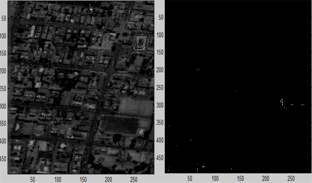
Figure 24.
Left: The source image. Right: The white points contain a target with t > 0.5 and corr > 0.8.
7. Conclusions
The paper presents two linear unmixing algorithms ROTU and CLUN to recognize targets in hyperspectral images where each given target’s spectral signature can be located in a sub- or above pixel. The CLUN algorithm is based on automatic extraction of features from the target’s spectrum. These features separate the target from the background. The ROTU algorithm is based on embedding the spectra space into a special space by random orthogonal transformation and by examining the statistical properties of the embedding’s result. In addition, we also compute the portion of the target’s material in the detected pixel (fractional abundance).The ROTU algorithm works well and fast if the spectra of the sought after target has sparse derivatives. It also works well if the fractional abundance of the target was 10, 30, 70 and 90%. It also detects sub- and above pixels with minimal false alarms. The CLUN algorithm works better but slower since it needs training phase and does background modeling.
References
- Madar, E. Literature Survey on Anomaly Detection in Hyperspectral Imaging; Research Report; Technion: Haifa, Israel, 2009. [Google Scholar]
- Averbuch, A.; Zheludev, M.; Zheludev, V. Unmix and target recognition in hyperspectral images, 2011; submitted.
- Spectral Imaging Ltd. Specim Camera; 2006. Available online: http://www.specim.fi/ (accessed on 1 February 2012).
- Bioucas-Dias, J.; Plaza, A. An Overview on Hyperspectral Unmixing: Geometrical, Statistical, and Sparse Regression Based Approaches. Proceeding of 2011 IEEE International Geoscience and Remote Sensing Symposium (IGARSS), Vancouver, BC, Canada, 24–29 July 2011; pp. 1135–1138.
- Bioucas-Dias, J.; Plaza, A. Hyperspectral unmixing: Geometrical, statistical and sparse regression-based approaches. Proc. SPIE 2010, 7830, 78300A-78300A-15. [Google Scholar]
- Manolakis, D.; Shaw, G. Detection algorithms for hyperspectral imaging applications. IEEE Signal Proc. Mag 2002, 19, 29–43. [Google Scholar]
- Manolakis, D.; Marden, D.; Shaw, G. Hyperspectral image processing for automatic target detection applications. Lincoln Lab J 2003, 14, 79–114. [Google Scholar]
- Settle, J.J. On the relationship between spectral unmixing and subspace projection. IEEE Trans. Geosci. Remote Sens 1996, 34, 1045–1046. [Google Scholar]
- Chang, C.I. Hyperspectral Imaging: Techniques for Spectral Detection and Classification; Kluwer Academic: New York, NY, USA, 2003. [Google Scholar]
- Common, P. Independent component analysis: A new concept. Signal Process 1994, 36, 287–314. [Google Scholar]
- Hyvarinen, A.; Karhunen, J.; Oja, E. Independent Component Analysis; John Wiley & Sons Inc: New York, NY, USA, 2001. [Google Scholar]
- Bayliss, J.D.; Gualtieri, J.A.; Cromp, R.F. Analysing hyperspectral data with independent component analysis. Proc. SPIE 1997, 3240, 133–143. [Google Scholar]
- Nascimento, J.M.P.; Bioucas-Dias, J.M.P. Does independent component analysis play a role in unmixing hyperspectral data? IEEE Trans. Geosci. Remote Sens 2005, 43(1), 175–187. [Google Scholar]
- Ifarraguerri, A.; Chang, C.I. Multispectral and hyper-spectral image analysis with convex cones. IEEE Trans. Geosci. Remote Sens 1999, 37, 756–770. [Google Scholar]
- Boardman, J. Automating Spectral Unmixing of AVIRIS Data Using Convex Geometry Concepts. Proceedings of the Fourth Annunl Airborne Gcoscicnce Workshop, Washington, DC, 25–29 October 1993; pp. 11–14.
- Craig, M.D. Minimum-volume transforms for remotely sensed data. IEEE Trans. Geosci. Remote Sens 1994, 32, 542–552. [Google Scholar]
- Bateson, C.; Asner, G.; Wessman, C. Endmember bundles: A new approach to incorporating endmember variability into spectral mixture analysis. IEEE Trans. Geosci. Remote Sens 2000, 38, 1083–1094. [Google Scholar]
- Winter, M.E. N-FINDR: An algorithm for fast autonomous spectral end-member determination in hyperspectral data. Proc. SPIE 1999, 3753, 266–275. [Google Scholar]
- Nascimento, M.P.; Bioucas-Dias, M. Vertex component analysis: A fast algorithm to unmix hyperspectral data. IEEE Trans. Geosci. Remote Sens 2005, 4, 898–910. [Google Scholar]
- Dobigeon, N.; Moussaoui, S.; Coulon, M.; Tourneret, J.-Y.; Hero, A.O. Joint Bayesian endmember extraction and linear unmixing for hyperspectral imagery. IEEE Trans. Signal Process 2009, 57, 4355–4368. [Google Scholar]
- Moussaoui, S.; Carteretb, C.; Briea, D.; Mohammad-Djafaric, A. Bayesian analysis of spectral mixture data using markov chain monte carlo methods. Chemometr. Intell. Lab 2006, 81, 137–148. [Google Scholar]
- Arngren, M.; Schmidt, M.N.; Larsen, J. Bayesian Nonnegative Matrix Factorization with Volume Prior for Unmixing of Hyperspectral Images. Proceedings of IEEE Workshop on Machine Learning for Signal Processing (MLSP), Grenoble, France, 2–4 September 2009; pp. 1–6.
- Cristianini, N.; Shawe-Taylor, J. Support Vector Machines and Other Kernel-Based Learning Methods; Cambridge University Press: Cambridge, UK, 2000. [Google Scholar]
- Burges, J.C. A tutorial on Support Vector Machines for pattern recognition. Data Min. Knowl. Disc 1998, 2, 121–167. [Google Scholar]
- Duda, R.O.; Hart, P.E.; Stork, D.G. Pattern Classification; John Wiley & Sons Inc: New York, NY, USA, 2001. [Google Scholar]