Recovery of Forest Canopy Parameters by Inversion of Multispectral LiDAR Data

Abstract

We describe the use of Bayesian inference techniques, notably Markov chain Monte Carlo (MCMC) and reversible jump MCMC (RJMCMC) methods, to recover forest structural and biochemical parameters from multispectral LiDAR (Light Detection and Ranging) data. We use a variable dimension, multi-layered model to represent a forest canopy or tree, and discuss the recovery of structure and depth profiles that relate to photochemical properties. We first demonstrate how simple vegetation indices such as the Normalized Differential Vegetation Index (NDVI), which relates to canopy biomass and light absorption, and Photochemical Reflectance Index (PRI) which is a measure of vegetation light use efficiency, can be measured from multispectral data. We further describe and demonstrate our layered approach on single wavelength real data, and on simulated multispectral data derived from real, rather than simulated, data sets. This evaluation shows successful recovery of a subset of parameters, as the complete recovery problem is ill-posed with the available data. We conclude that the approach has promise, and suggest future developments to address the current difficulties in parameter inversion.

1. Introduction

Laser scanning has become leading edge technology for the acquisition of topographical data and for mapping the Earth’s surface. Recent technological advances in electronic devices for fast digitising and storing of mass data have made it possible to digitally sample the entire laser pulse echo as a function of time. Typical waveform LiDARs are particularly attractive for forest applications as a laser beam can penetrate a forest’s structure, and so provides 3-dimensional information at a high point density of the intensity of the return signal, but only at one specific wavelength. For over a decade waveform LiDAR has been used to retrieve forest parameters such as tree height, crown diameter, number of stems, stem diameter and basal area [1,2]. LiDAR remote sensing has also been widely used to infer estimates of vegetation structure and biomass [3,4] at various scales ranging from single-tree level [5] to landscape level depending on the application and/or the LiDAR system used. What is missing with current LiDAR technology is the ability to measure a suite of wavelengths which are sensitive not only to structural elements but also to the spectral reflectance properties of those elements which are in turn indicative of physiological changes within the leaves [6]. Whilst current multispectral remote sensing approaches enable monitoring ecosystems productivity related functions at synoptic time and space scales through observation and understanding of ecosystem carbon-related spectral responses, passive systems suffer from viewing mostly only the top of the canopy, both obscuring and shading the understorey and ground that lie beneath the canopy. There is a real need for an active (laser) system capable of measuring both structural parameters and physiological changes through the depth of the canopy, including the understorey.

Therefore, a multispectral canopy lidar (MSCL) would provide much needed information on the vertical distribution of physiological processes which in turn would provide greater detail on actual carbon sequestration as well as existing stocks, with the spectral contrast further allowing separation of the ground from canopy returns. This will inform our understanding of the seasonal dynamics of ecosystem carbon uptake in response to environmental drivers such as water, temperature, light and nutrient availability.

In conjunction with sensor development, we are investigating improved methods to better interpret single and multispectral LiDAR data, which are the principal contributions of this article. Previously, we presented an effective approach to process full waveform LiDAR data [7] with the capability to resolve and better detect low amplitude surface returns and improve resolution. We now show how full waveform processing using Bayesian techniques can provide a variable dimension model of the tree or forest canopy structure, and then extend these ideas to process across different wavelengths so that our inference is simultaneous on depth and wavelength. We evaluate our approach on simulated and real data, on photon count and pulsed intensity laser systems. We then summarise some of the necessary steps that need to be taken to design and exploit multi- or hyper-spectral LiDAR systems.

2. Forest Monitoring Using LiDAR Data

LiDAR is used primarily for recovering depth, and by extension 3D imagery when the sensor is scanned or a 2D focal plane sensor is employed. Mallet and Bretar [8] provide a comprehensive survey of both air and space borne LiDAR systems that can be used to provide full waveform data with particular emphasis on data recovery from wooded areas, although they also include examples from mountains and urban regions. Leuwen and Nieuwenhuis [2] complement this article by reviewing the recovery by LiDAR of structural parameters from forest areas. The key parameters they describe are tree or canopy height, leaf area index, fractional cover, foliage height profile, biomass and tree volume, terrain and terrain slope, and by extension, species classification.

In evaluating structural properties from LiDAR data, a standard approach has been to assume that the instrumental response is known, usually modeled by a Gaussian, and to decompose the waveform into a series of such Gaussians that indicate the presence of “apparent” reflecting surfaces. This technique was applied to the Laser Vegetation Imaging Sensor (LVIS) data [9] to recover forest structural characteristics such as stem diameter, basal area and above ground biomass, using known regression relationships between these and measured canopy height, height of median energy and the energy ratio in the ground return [10]. The problem was to determine the number and position of the Gaussians by finding inflection points, but this is difficult in the presence of noise as it relies on derivatives, even if the data is smoothed. In later work [11], they extracted a number of parameters (centroid, signal beginning, end, etc.) from full waveform LiDAR to measure tree height, again by learnt allometric relationships. Similarly, Jaskerniak et al. [12] fitted bimodal and occasionally multimodal distribution functions to interpret the understorey and overstorey of a vegetation profile in eucalyptus forest. However, there was an a priori assumption that the number of layers of the forest canopy was known, i.e., that the number of modes was predetermined.

Mallet et al. [13] described an approach to allow variation in the number of modes using reversible jump Markov chain Monte Carlo (RJMCMC) inference; this is a dimension varying strategy we have previously employed [7] and continue here. Further, they also applied a switching strategy between three different structural models based on tree shape; this could then be convolved with a fixed instrumental response. They employed a perturbation strategy to alter the parameters of the structural alternatives, i.e. within model parameter variation. In this paper, we do not switch shape models. We use a layered model strategy that is general, in that asymmetric shapes for example, are represented by closely spaced discrete convolved responses of different amplitude. Further we also address the problems of spectral variation and mixture of materials (e.g., leaf, bark, soil).

Several researchers (e.g., [14–16]) have cited and discussed the use of spectral analysis of leaves to estimate biochemical content, and further comment that the main photosynthetic components, including chlorophyll a and b (C_ab), are effective indicators of the health of the forest canopy, and whether the canopy is under physiological stress. Variations in chlorophyll content are also dependent on species type, needle age and the illumination conditions within the canopy. However, measuring the spectral reflectance of foliage at canopy, as opposed to leaf scale, is very difficult as the spectrum is confounded by the proportion of woody elements such as trunk, branch and twig elements, and in an integrated passive sensing instrument this can also be affected by a proportion of soil reflectance from below the canopy. A key difference between the spectral characteristic of photosynthetic vegetation (PV) and non-photosynthetic vegetation (NPV) and litter within the canopy is the presence of the “red edge”, a steep rise in reflectance between 680 nm and 730 nm, which survives the superimposition of PV and NPV signatures.

The Normalized Differential Vegetation Index (NDVI) is formed from the normalized reflectance values either side of the red edge, which discriminates between live green and other canopy material. Subject to the caveat that the NDVI can be affected by both the relative proportion of PV and the health of that vegetation, it has been found to correlate reasonably well with above ground biomass, leaf area index (LAI) and the fraction of absorbed, photosynthetically active radiation (FAPAR). However, it does not capture fine temporal and spectral variation of physiological parameters [17]. The Photochemical Reflectance Index [18] (PRI) uses the reflectance at two narrow bands centred on 531 nm (or 532 nm) and 550 nm (or 570 nm) to quantify vegetation Light Use Efficiency (LUE), via the change in state of the xanthophyll cycle pigments. As noted in [16,18] the relative photosynthetic rates can only be reliably determined “if issues of canopy and stand structure can be resolved”. If simple indices such as NDVI and PRI are not sufficient to distinguish between the health of vegetation and the relative proportions of PV and NPV, then what additional information is required? The first option is to make use of a priori data that might be used to constrain the inversion problem. 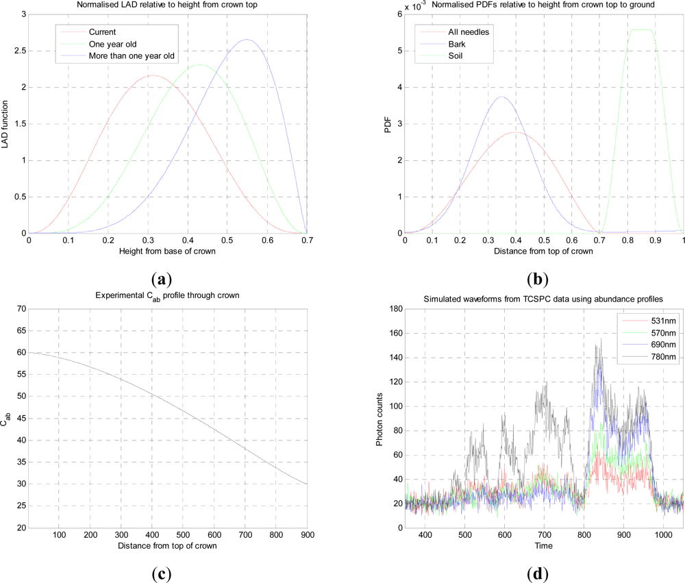For example, in interpreting data from a Sitka Spruce canopy in Scotland (which occurs in one of our proposed test areas) we can use a priori models such as the vertical and horizontal distributions of needle area density [19,20] approximated by a two dimensional Beta distribution within a homogeneous ellipsoidal crown, which can be linked quite effectively to radiative transfer models. Malenovsky et al. [21] have considered the effect of different a priori assumptions on reflectance parameters using the DART model as a tool for parameter recovery, i.e., leaf only, leaves trunks and first order branches, and the addition of woody twigs. As expected, the inclusion of woody elements does indeed perturb the recorded values of the NDVI and another index, the AVI (Angular Vegetation Index), and they conclude not surprisingly that a priori knowledge is needed to solve the inversion problem. Alternatively, one can combine LiDAR data with a passive hyperspectral imaging system (e.g., [22,23]). In a simple case, the two information sources may provide assumed, independent structural and biochemical and structural forest properties. However, this assumes both temporal and spatial registration of the source data. This has rarely been the case as the data often come from different platforms. Further, the spectral signature is integrated over all depth rather than a function of depth and so loses information. This impels the development of multispectral LiDAR systems for the monitoring of forest canopy properties [24,25].

The recently developed and active airborne photon counting LiDAR system called SIMPL (Slope Imaging Multi-polarization Photon Counting Lidar) [26] is a dual channel system that measures at two wavelengths (532 nm and 1,064 nm) in parallel and perpendicular polarization channels, and is a time-correlated single photon counting system deployed in an airborne platform. In this paper, we also use a time-correlated photon counting LiDAR system to acquire measurements from a small sample conifer to illustrate our techniques. Moving beyond a small subset of wavelengths and simple reflectance ratios, an exciting prospect is to use a super continuum laser to provide a hyperspectral LiDAR system that can capture a vertical profile of spectral data that could possibly resolve structural, material and biophysical parameters in a single instrument. Chen et al. [27] experimented with a super continuum laser to measure NDVI on Norway Spruce with only two of the possible wavelengths. Later they combined a monochromatic LiDAR with a spectrometer using the same supercontinuum source [28] to create a ‘virtual’ hyperspectral system. This was used to differentiate between materials including trunk/wood and needles, but such a system does provide a full spectrum that could be used for further analysis. Of particular interest, in the conclusions they talked of the potential to retrieve target chlorophyll content which is a subject of this paper.

In Section 3, we describe a preliminary experiment that shows the potential of multispectral LiDAR to measure simple indices that can be related to tree stress. In Section 4, we formulate a modelling and inversion framework that can be applied to ether single or multiple wavelength LiDAR data. However, the data presented in Section 3 is not suitable for full parameter inversion, so in Section 5, we apply these methods to recover a variable dimension structural model from a single wavelength signal, using time-correlated single photon counting data acquired by our own LiDAR system from a small conifer at a range of 330 m. We then extend the approach to recover structural and photochemical parameters in Section 6, using a simulated set of waveforms based on the real structure of the conifer measurement. Finally we summarise our work and suggest future developments in Section 7.

3. Measuring Multi Spectral Data

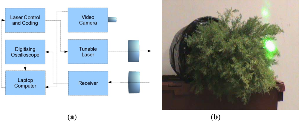
A joint research contract between the University of Edinburgh and SELEX-GALILEO was held during 2008, with the aim of conducting a preliminary trial to assess the capability of a bread board MSCL instrument to distinguish between stressed and unstressed evergreen conifer trees (Cupressus macrocarpa). Unstressed samples were watered regularly over that period, but the stressed samples had the root ball encased in plastic and were not watered. Measurements were taken of both stressed and unstressed trees with a tunable laser (500–550 nm and 690–800 nm) using a optical parametric oscillator (OPO) as a resonant laser cavity. The return energy was focused onto the detector and a fast digitizing oscilloscope sampled the signal at up to 10MSamples·s⁻¹. An instrumental response was obtained for each spectral channel by reflection from a white card immediately previous to any tree measurement to allow for calibration of variations in power as a function of time and wavelength.

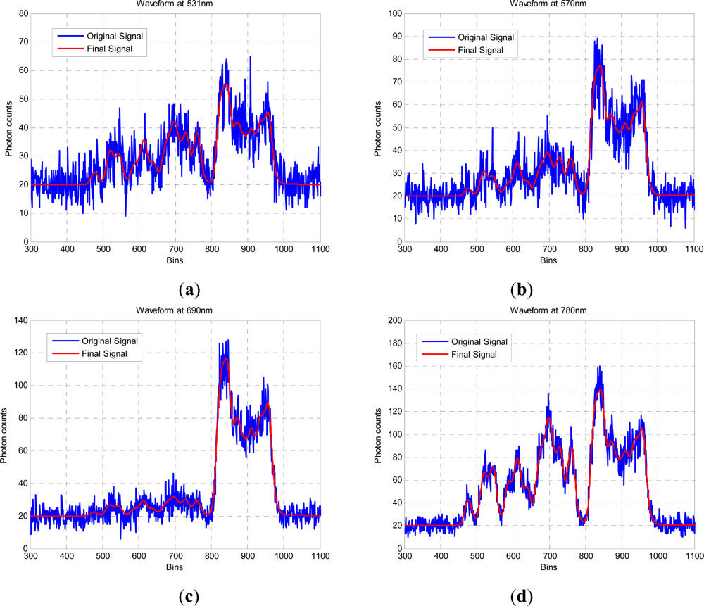
A schematic illustration of the system is given in Figure 1(a) and a picture of the laser signal on the conifer in Figure 1(b). The measurements were taken in two sets of two wavelengths (531/550 nm and 690/780 nm) to mimic the recording or PRI and NDVI data, rather than measuring all four channels simultaneously. As discussed in Section 2, the utility of PRI and NDVI wavelengths for understanding light use efficiency and light absorption in a forested environment is very well established, and we have ∼15 years experiences of passive data analysis. The two sets of signals are not registered either spatially or temporally and the recorded measurements were averaged over 16 samples.

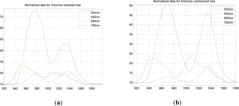
Figure 2(a,b) shows the normalized response data for both stressed and unstressed trees for all four wavelengths, in which the lower two and upper two wavelengths are registered temporally and on the same part of the tree, but this is not the case for the two sets of data. However, the two trees sampled were the same age with very similar structures. The actual mix of foliage and branch observed would have differed slightly but the same area of material was illuminated by the laser.

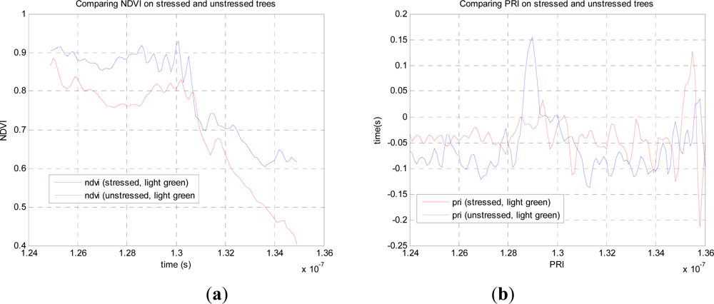
From this data we can compare the stressed and unstressed data in Figure 3. Defining the NDVI as (R₇₈₀−R₆₉₀)/(R₇₈₀+R₆₉₀), we notice a drop in the canopy from 0.89 (unstressed) to 0.76 (stressed) at the point of maximum difference, 1.28.10⁻⁷ s. Over the canopy volume, the PRI, defined as (R₅₃₂−R₅₅₀)/(R₅₃₂+R₅₅₀), is far less consistent, and it is difficult to come to a meaningful conclusion. These results can be compared with recent airborne measurements on conifer forests by Hernandez-Clemente et al. [29] Similar to the results presented here, they too observed a substantial drop in NDVI for the ‘stressed’ crown, from 0.71 to 0.55, but we cannot compare values exactly as these are different species, different degrees of stress, different mixtures of needles and other material. In short, this preliminary experiment demonstrates the potential, but is insufficient for further analysis, so we use our own data augmented by simulations in what follows.

3. Formulating the Modelling and Inversion Framework

In modelling trees or forest canopies, we have limiting choices between a full structural mesh that can represent leaf, wood or ground elements by polygons with parameters to define the reflectance (and possibly absorption and transmittance) function [30,31] and structurally homogeneous models that represent the canopy, for example, by a medium with known wavelength dependent entry and exit probabilities and turbid medium extinction coefficients. Models such as FLIGHT, a widely used model of light transport for the optical domain, based on Monte Carlo solution of radiative transfer [32], use a hybrid structure where the crowns are turbid media, but rays are traced between different structural elements, e.g., from crown to crown or crown to ground. Together with a leaf optical properties model such as PROSPECT [33] to determine the canopy spectral reflectance, and measured spectral variation of bark and reflectance properties, radiative transfer models provide powerful tools for simulation, and to some extent evaluation of inversion algorithms. A full and thorough comparison of these can be found in the series of RAMI benchmarking exercises [34].

In modelling radiative transfer, we have to balance the complexity of the model against the nature of the sensed data, and the likelihood of parameter recovery. On the one hand, it is wholly intractable and not useful to recover the parameters of each leaf, although that can be represented in a graphical model. On the other hand, representation of the canopy by a homogeneous medium has no value as we seek to recover variation of structure and photochemistry as a function of canopy penetration. Even a complex graphical model does not fully account for absorption, multiple reflection and transmission, so where should one “draw the line” in considering multiple reflection? If we consider for example the model of Smolander and Stenberg [35] for shoot scattering in Scots pine, we can see that the delay between hits is very short as the needles are densely packed, and that longer delays are more prevalent in either flat leafed species or where the incident photons hit woody material. Disney et al. [36] have also investigated the contribution to the measured signal of secondary and higher order scattering events in their own and the Smolander-Stenberg shoot designs, and show that in each case the signal contribution drops off rapidly in amplitude, with 76% from the primary reflection at the appropriate nadir angle of incidence. Hancock [37] further confirms in a series of simulations that the principal effect of multiple scattering is to increase reflectance, rather than change the shape of the waveform. Therefore, and for reasons of tractability, we further assume a Lambertian reflectance model.

A single LiDAR footprint provides no information on (x,y) spatial location, so this leads us to assume homogeneity within the (x,y) planes of the footprint, or at least an integrated measurement parameter. We consider the full waveform LiDAR signals as independent measurements, we do not consider dependencies between laser footprints that are adjacent spatially on the earth’s surface. We have considered a fixed layer canopy representation similar to Garcia-Haro et al. [38], but this has two drawbacks. First, it introduces needless complexity if we try to recover layer parameters for which no or little data exists, e.g., gaps in the canopy as a function of depth (z). Second, any fixed, layered model is not matched to the LiDAR response, that is to say the maxima in the scattering profile will not in general coincide with predefined layer positions. Therefore we will use a variable (number, positions and amplitudes) dimension model to represent the canopy derived from the structural LiDAR signal. This has the advantages of adapting to the structure of each signal and reducing the model dimension for accurate representation of the underlying canopy or tree structure. Thus the signal is sampled regularly in depth by the sensor, but our representation approximates this by a smaller, finite set of irregularly spaced layered approximations that best represent the canopy structure.

Hence, there are L full LiDAR waveforms, each of length N bins (i,1…N), one for each wavelength. It is assumed that each of the L waveforms is recorded from the same structure at the same time, the spectral channels are co-axial as in our own sensors. In each bin, y_z,l, is a sample from a Poisson distribution to represent variation in the count data. The known instrumental function is represented a piecewise exponential [7]. We represent the multispectral LiDAR response by a mixture model [39] consisting of discrete returns from several aggregated surfaces. This does not suggest that a tree canopy can truly be represented by discrete layers of no thickness, but we demonstrate that this provides an excellent approximation to the real data, certainly within the limits of typical noise levels.

Hence,

$$p(y_{z,\lambda }|k,\omega ,\varnothing )={\sum }_{m,1}^k{\sum }_{l,1}^R{\omega }_{z,l}f(y_{z,\lambda }|k,{\varnothing }_{m,l})+B_{\lambda }$$

(1)

where

• y_z,λ is the photon count within a bin, indexed by (z,λ) defining the distance and wavelength.
• k is the variable number of layers.
• R defines the number of materials (e.g., needles, bark, soil) of the mixture. We shall assume this is fixed, i.e., the number of possible materials is known.
• Φ_m,l is the parameter vector of the m^th layer response for the l^th component of the mixture. ϕ_l = [ϕ_z, ϕ_λ], where ϕ_z defines the temporal, and ϕ_λ the spectral signature. The temporal signature is defined by the instrumental response, which we assume is not wavelength dependent, or can be calibrated to adjust for wavelength dependence. The spectral signature is defined by the Prospect model.
• ω_z,l defines the fraction or abundance of l^th component at distance, z. These satisfy the conditions, ω_z,l > 0 for all z, l and ${\sum }_{l,1}^R{\omega }_{z,l}=1$.
• B_λ is a background and dark photon count level, which we assume is constant in all bins at the same wavelength, but varies across wavelengths.
• p is a conditional probability distribution function.

φ_z is defined by

β	area parameter
z0	positional parameter (depth)
Bλ	background parameter

The spectral response depends on both the relative abundance and the spectral signature of each mixture component. We use the Prospect to model the leaf spectra,

φλ	{leaf}
N	leaf structural parameter
Cab	concentration of chlorophyll a and b
Cw	equivalent water thickness
Cm	concentration of dry matter
Cbrown	concentration of brown pigments
Car	concentration of carotenoids

For measurements in the visible and near infra red regions of the spectrum, the key constituents are C_ab and C_m, as the others have lesser or no effect. We use prototypical fixed spectra for the other mixture components, φ_x, taken from [40,41], effectively look-up tables that can be chosen to suit the bark and soil properties. If not known, then this would provide yet another parameter to add to the ill-posed nature of the problem, discussed in Section 5.1.

Given a set of data, and a variable dimension mixture model, we would apply Bayesian inference to recover the number of layers and the parameter vector, φ_m,l, for each layer. For this inference, we apply a Reversible Jump Markov Chain Monte Carlo (RJMCMC) algorithm. We have already employed both MCMC and RJMCMC algorithms to successfully locate the positions and amplitudes of all returns in full waveform LiDAR data [7] and the reader is referred to that paper for a full discussion. However, this paper extends the discussion to define appropriate models for the forest canopy parameter inversion problem, and considers the use of multispectral data to recover biochemical parameters for the first time.

The value y_z,λ recorded in each bin is considered as a random sample from a Poisson distribution with intensity that depends on the model parameters.

$$P_o(y_{z,\lambda }|k,\omega ,\varphi )=e^{-p(y_{z,\lambda }|k,\omega ,\varnothing )}\frac{p{(y_{z,\lambda }|k,\omega ,\varnothing )}^{y_{ij}}}{y_{z,\lambda }!}$$

(2)

Furthermore, assuming that the observations recorded in each channel are conditionally independent given the values of the parameters, and each record is an independent measurement, the joint probability distribution of y is defined as

$$L(y|k,\omega ,\varphi )={\prod }_{z,1}^Z{\prod }_{l,1}^R{e}^{-p(y_{z,\lambda }|k,\omega ,\varnothing )}\frac{p{(y_{z,\lambda }|k,\omega ,\varnothing )}^{y_{z,\lambda }}}{y_{z,\lambda }!}$$

(3)

As it is not possible to have negative values of y_z,λ, and because the product tends to zero, we minimize −2lnL(c/ϕ) as is common practice. The last of the three terms, ln(y_z,λ!), is omitted as it is constant.

$$-2\text{ln}(L(y|k,\omega ,\varphi ))=2{\sum }_{z,1}^Z{\sum }_{l,1}^R\left[p(y_{z,\lambda }|k,\omega ,\varnothing )-y_{z,\lambda }\mathit{ln}\left(p(y_{z,\lambda }|k,\omega ,\varnothing )\right)\right]$$

(4)

To make inferences about the dimension, k, and the consequent parameter vector, φ, of our model given the data, y, the likelihood, L, is combined with prior information, P. This is summarised in a posterior, or target distribution,

$$\pi (k,\omega ,\varphi |y)=\frac{L(k,\omega ,\varphi |y)P(k,\omega ,\varphi )}{\int L(k,\omega ,\varphi |y)P(k,\omega ,\varphi )\delta (k,\omega ,\varphi )}$$

(5)

At each iteration, there are two steps, a parameter updating step, with fixed dimension, and a dimension-changing step that allows jumps between different numbers of returns. This latter increase or decrease can be achieved by a birth of a new, or splitting of an existing return, or a death of an existing, or a merging of two existing returns. Hence a single ‘sweep’ of an ideal Markov chain for all the parameters of interest is

Algorithm 1. Updating of parameters in a multispectral RJMCMC algorithm

Fixed dimension (known number of layers, k): Update φz Update area vector, β Update position vector, zo Update φλ Update abundance vector, ω Update Prospect model, Cab and Cm Update background values, Bλ

Change of dimension, k Birth or split of return/layer, increments k Death or merge of two returns/layers, decrement k

Algorithm 1. Updating of parameters in a multispectral RJMCMC algorithm

Fixed dimension (known number of layers, k): Update φz Update area vector, β Update position vector, zo Update φλ Update abundance vector, ω Update Prospect model, Cab and Cm Update background values, Bλ

Change of dimension, k Birth or split of return/layer, increments k Death or merge of two returns/layers, decrement k

A proposed move is accepted with the general probability,

$${\alpha }_m(k,\omega ,\varphi ,k^{\prime },{\omega }^{\prime },{\varphi }^{\prime })=\mathit{min}\left\{1,\frac{\pi (k^{\prime },{\omega }^{\prime },{\varphi }^{\prime }|y)}{\pi (k,\omega ,\varphi |y)}X\frac{q_m(k^{\prime },{\omega }^{\prime },{\varphi }^{\prime },k,\omega ,\varphi )}{q_m(k,\omega ,\varphi ,k^{\prime },{\omega }^{\prime },{\varphi }^{\prime })}\right\}$$

(6)

where α_m is the acceptance probability for a move from (k,ω,ϕ) to (k’,ω’,ϕ’), π is the target distribution, y the data distribution, q_m the proposal distribution, and the subscript m denotes the type of move. For parameter updating at a fixed number of returns, this reduces to the conventional Metropolis-Hastings probability,

$$\alpha (\varphi ,\omega ,{\varphi }^{\prime },{\omega }^{\prime })=\mathit{min}\left\{1,\frac{\pi ({\omega }^{\prime }{\varphi }^{\prime }|y)}{\pi (\omega ,\varphi |y)}\times \frac{{\text{q}}_{\text{m}}({\omega }^{\prime },{\varphi }^{\prime },\omega ,\varphi )}{{\text{q}}_{\text{m}}(,\omega ,\varphi ,{\omega }^{\prime },{\varphi }^{\prime })}\right\}$$

(7)

The birth/death and split/merge moves require a change of dimension and, therefore, RJMCMC is used. Considering the birth death moves, then the acceptance probability becomes

$${\alpha }_m(k,\omega ,\varphi ,k^{\prime },{\omega }^{\prime },{\varphi }^{\prime })=\mathit{min}\left\{1,\frac{\pi (k^{\prime },{\omega }^{\prime }{\varphi }^{\prime }|y)}{\pi (k,\omega ,\varphi |y)}\times \frac{{\text{r}}_{\text{m}}({\omega }^{\prime },{\varphi }^{\prime },\omega ,\varphi )}{{\text{r}}_{\text{m}}(\omega ,\varphi ,{\omega }^{\prime },{\varphi }^{\prime })}\times \left|\frac{\delta ({\omega }^{\prime },{\varphi }^{\prime })}{\delta (\omega ,\varphi ,u)}\right|\right\}$$

(8)

where r_m(x) is the probability of choosing move type m when in state (ω,ϕ), u is a vector of continuous random variables which ensures the reversibility of the deterministic function ϕ’,h(ω,ϕ, u), which allows the move to a higher-dimensional space and q(u) is the probability density function of u. The Jacobian term, arising from the change of variable from (ω,ϕ, u), to (ω’,ϕ’), ensures the dimension balancing condition that allows reversible jumps between different dimensions of k.

4. Determining Structure from Single Wavelength LiDAR Data

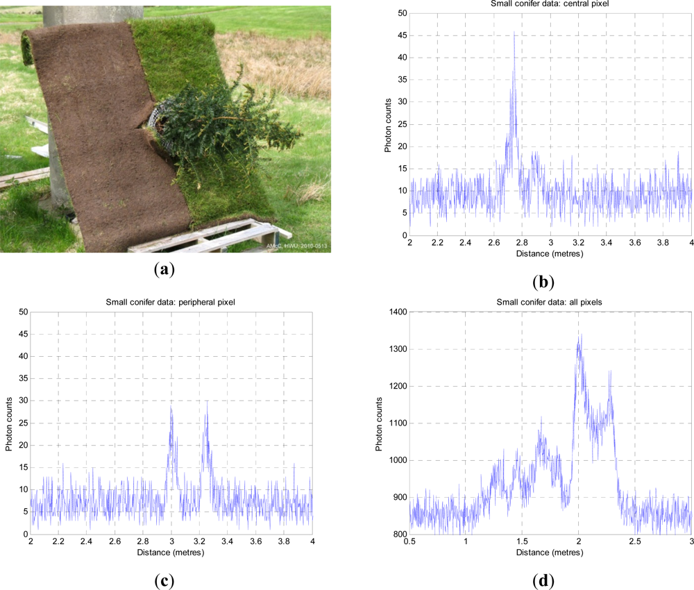
To demonstrate the recovery of structural data from full waveform LiDAR we used the system described in [42] to measure a 10 by 10 matrix of full waveforms of a small conifer on a bright day in high white cloud, as shown in Figure 4. The stand-off distance was ∼325 m from the baseboard. This resulted in a beam spot size at the target of approximately 14 mm. The baseboard was half soil, half grass, with a side dimension of 1,250 mm. The height of the conifer was 1.10 m. The laser wavelength was 842 nm, repetition rate 3 MHz and illumination power at the target about 50 μW on average. As the laser source was low, each measurement used a 10s dwell time, and was repeated at temporal resolutions of 4 ps and 16 ps.

If we look at Figure 4(b), it is clear that little light penetrates to ground level, even in such a small, sparsely foliated specimen, but we can see a number of peaks below (right) of the first return. In Figure 4(c), we observe structure from the side of the tree and the ground beneath. Figure 4(d) shows the integrated return from all 100 pixels of the tree image and is equivalent to a wider footprint image of the tree as a whole, although the background level is higher. In the integrated plot, the three tier structure of the tree is very evident as the three leftmost peaks. The higher bimodal peak on the right is the ground return, distributed in depth as the LiDAR beam is not normal to the ground plane. The dip in the middle is where the ground is obscured below the tree.

We estimate the numbers, amplitudes and positions of the several “layers” in the conifer. We do not yet attempt to retrieve any biochemical parameters as there is no information about spectral variation. The aggregated counts shown in Figure 4(d) are a result of reflections from densely distributed needle, twig, branch, trunk and ground data, compounded by background counts and multiple reflections. We cannot say whether a given amplitude of return is due to a large area of low reflectivity, or a small area of high reflectivity, where reflectivity depends on material. We use non-informative priors on the number, position and amplitude/area of the returns. In summary, we recover a variable dimension layered model, tree height and layer area distribution, and a single sweep of the algorithm is now

Algorithm 2. updating of structural parameters only from a single wavelength

Fixed dimension (known layer positions): Update φz Update amplitude vector, β Update position vector, zo Update background values, Bλ

Change of dimension, k Birth or split of return/layer, increments k Death or merge of two returns/layers, decrement k

Algorithm 2. updating of structural parameters only from a single wavelength

Fixed dimension (known layer positions): Update φz Update amplitude vector, β Update position vector, zo Update background values, Bλ

Change of dimension, k Birth or split of return/layer, increments k Death or merge of two returns/layers, decrement k

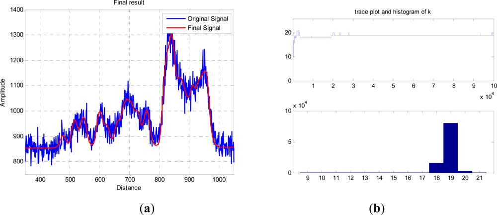
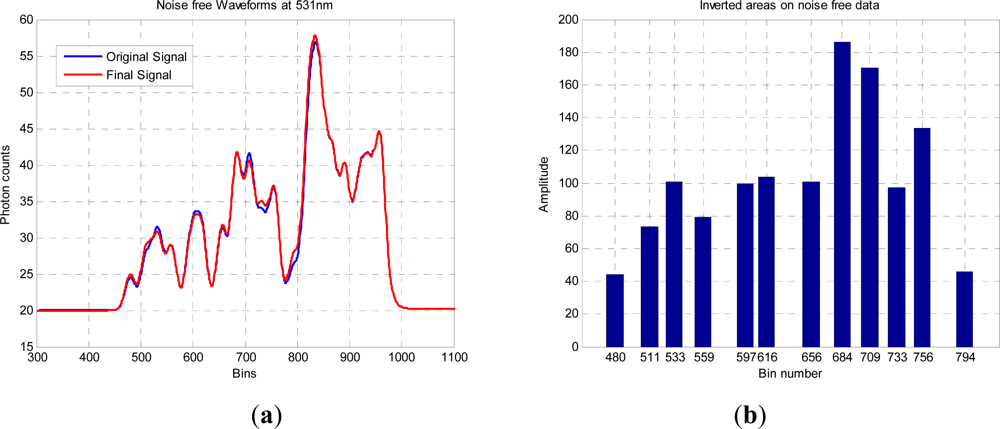
The red curve in Figure 5(a) shows an exemplary result of an RJMCMC chain having 10⁵ iterations, and allowing dimensional changes from 3 to 20 returns. The trace and final histogram of p(k|y) are shown in Figure 5(b) and the final parameter values, p(φ|k,y), for the most likely number of “layers” are tabulated in

Table 1. Positions and amplitudes of layers on the measured, 842 nm integrated LiDAR data from small conifer. The background level was estimated at 854.2 counts and the mean rms fitting error was 0.67 counts.

Position (bins)	478	517	547	601	626	662	686	706	729	759
Amplitude (counts)	48.6	108.1	116.0	141.1	75.9	97.6	157.5	145.0	124.2	141.7
Position (bins)	822	841	849	869	887	910	926	940	959
Amplitude (counts)	291.5	279.9	142.8	202.4	165.7	186.9	110.2	188.0	249.6

. Due to the random sampling and finite run length of the algorithm, different runs will produce different values for both k and the subsequent distribution of peaks and amplitudes, but in general the accumulated errors between the two curves are equivalent. For the most probable k = 19, the other parameters are tabulated below.

This is a purely structural measurement, so we do not recover physiological properties. Structural parameters such as height and biomass can be recovered from the measurements, and if appropriate by previously established regression relationships. For example, if we define the height as the separation between the minimum and maximum positions, then the separation is 440 bins of width 16 ps which corresponds to 1.06 m, allowing for the go-return path. This height is relative to the furthest ground position and equates to the known size and geometry of the tree and baseboard. The amplitudes of return are more problematic; as noted above, we would need to assume a known mixture model to measure leaf area index, and model the transmission path effectively. If we measure a continuous canopy, then we can assume a model of penetration where the incident light at each layer is reduced by the already reflected or absorbed light at higher layers. In this experiment, however, as the single tree is scanned as an image and the several counts integrated, the bulk of the returns at lower levels of the tree are from the sides rather than from penetrations into the tree at the centre. (The same would be true if we had deliberately increased beam divergence to give a wide footprint.)

5. Determining Structure and Photochemical Properties from Multi Spectral LiDAR Data

5.1. Spectral Data and the Ill-Posed Problem

With reference to Algorithm 1, we could in theory apply simultaneous inversion of all parameters of interest. This involves the computation of likelihood functions on all wavelengths for every parameter proposal, and has in general great complexity defined both by the number of iterations in the Markov chain, and the number of bins in the histograms of photon counts. Further, we observe that in principle, the positions (but not the amplitudes) of the returns should be identical if all are aligned, as all should impact the same surfaces, at least to the first reflection. However, we cannot hope to recover all parameters unambiguously from four wavelengths, which we consider here as those necessary to recover NDVI and PRI, as the likelihood function can have many maxima for different values of abundance, C_ab and C_m.

To demonstrate the complex nature of parameter inversion, consider the variation of NDVI with different values of abundance and C_ab, illustrated in Figure 6, using spectral data generated from PROSPECT and Spruce bark. We do not consider variation in bark spectra or leaf C_m. This clearly shows that NDVI can assume any value for abundance dependent on the modelled density of C_ab, or vice versa. In principle, with appropriate proposal management, we might explore loci of maximum likelihood, but that may not be tractable and is beyond the current scope. Rather, we investigate the recovery of two subsets of structural and photochemical parameters as defined in Section 5.2.

5.2. Recovering Area and Photochemical Parameters from Multispectral Data

We use the same data to demonstrate the recovery of area and photochemical parameters as Section 4. As we only have real, single waveform data, we create a synthetic set of full waveform data shown in Figure 7(d) at the four wavelengths of interest, i.e., 531 nm, 570 nm, 690 nm and 780 nm. To do this we first use RJMCMC to define a layered model as described in Section 4. We then define an abundance model using the data of Wang and Jarvis [20] to model the distribution of current, first and second year leaves, and defining C_ab concentrations from Malenovsky [21]. We further assume that the overall proportion of NPV to PV returns is about 0.06, as measured by Hancock [37] in his simulations. This gives simulated abundance and C_ab profiles as shown in Figure 6. To generate the waveforms shown in Figure 7, we finally add Poisson distributed noise. We stress that these are not true distributions, but have some prior basis, and provide ground truth to evaluate the algorithm.

We can make some general observations on these spectra. First the ground return is assumed to be soil alone, so there is an increase in reflectance with wavelength because the soil reflectance is monotonically increasing. Examining the canopy, we have assumed predominant returns from needle rather than woody material, so that the peak at 531 nm and the dip in reflectance at 690 nm are observed even though some monotonically increasing bark reflectance is present.

The inversion process recovers background, positions and amplitudes from a single spectrum (780 nm) similar to Algorithm 2 (Stage 1), then fixes the dimension (k) and positions in a multispectral inversion (Stage 2). We have conducted experiments with many combinations of parameters, but demonstrate one example where the solution space is relatively stable. In addition to the structural measurement, we also measure C_ab as a function of canopy penetration. Hence, the process is summarized as follows,

Stage 1: Using a single wavelength: unknown number of layers, positions and amplitudes

Fixed dimension (known number of layers, k):

• Update φ_z
  • Update amplitude vector, β
  • Update position vector, z_o
• Update background values, B_λ

Change of dimension, k

• Birth or split of return/layer, increments k
• Death or merge of two returns/layers, decrement k

Stage 2: Using multiple wavelengths: known number of layers and positions

Fixed dimension (known number of layers, k, abundance vector, ω, and C_m):

• Update φ_z
  • Update area vector, A
• Update φ_λ
  • Update Prospect model, C_ab, for each layer
• Update background values, B_λ

There is a distinction between the calculation of the amplitude vector in a single waveform, which is related to the area and reflectance (and hence material) of the intersecting surfaces, and the area update in a multi spectral waveform, which depends on the known or current estimates of abundance and reflectance (from PROSPECT) to compute an amplitude in each waveform.

First we consider a noise free example. As stated above, we use non-informative priors on all the parameters of interests, and effectively recover the positions, areas and C_ab concentrations as a function of depth into the tree signature. The number of iterations of each chain was 4.10⁴ and we used a burn-in period of 10⁴, although this was not critical. As we can see from both the fitted waveform at 531 nm (actually the worst fit) and the recovered area values in Figure 8, the process recovers the overall structural distribution well, as was the case with the real data in Section 4. Of more interest is the recovery of the C_ab concentration in Figure 8(c). This shows that the profile is well recovered with a root mean square error of 1.96 ug·cm⁻², but of course this is on noise free data.

We next investigate the more realistic example of synthesized TCSPC waveforms in which Poisson noise is added to each bin of the histogram in accordance with mean photon count level of the bin, i.e., data such as that shown in Figure 7(d). In running repeated tests on noisy data we observe that as both synthesis and recovery are random processes, at each run we both create a different set of spectral signatures and run a different set of chains. Hence the recovered layer positions should not and do not correspond exactly between any two runs, even though in general the waveforms are well approximated by the parameter recovery. Otherwise the initial conditions and chain lengths were equivalent to the noise free experiments.

The first key observation from Figure 9 is that the areas and positions of the recovered layers, together with the assumed abundance values and the PROSPECT generated spectra model the raw data quite well, within the error of the generated noise distribution. This is one example, but the root mean square error is less than one count in all cases. In practice, the positions and corresponding areas can vary considerably, as the waveforms with noise may be fitted by several position, area, spectrum combinations. This can be seen in Figure 9(e,f), in which the complete set of recovered area and C_ab parameters are shown on single graphs. First, the area graph can be compared with the noise free example in Figure 8(b); in Figure 9(e) we can see that it captures the three layer structure of the conifer well but at this stage we have no real ground truth for comparison. The C_ab data of Figure 9(f) has been fitted by a polynomial of the third order (although this is not significant) and this can be compared to both the noise free example and the ground truth which is shown in the same graph. The parameter inversion does recover the decreasing trend of the C_ab profile well, but is clearly some distance above the regression fit, and there is considerable scatter in the recorded points with a residual norm of approximately 100 counts. This illustrates again how difficult the problem is with only four spectral measurements. If one looks at the likelihood function as a function of C_ab variation, it is relatively flat, i.e., a slight variation in C_ab estimation does not alter the synthesized waveform in comparison with the added noise. Again this suggests that we may need additional spectral data to fully resolve the problems of spectral un-mixing combined with physiological parameter recovery. Here, we were only interested in investigating wavelengths that were directly related to gross primary productivity but are exploring other frequencies that relate to water content of vegetation and fluorescence. The exact choice of these wavelengths depends primarily on optimal recovery of the Prospect parameters, other material parameters, together with system parameters including for example the detector spectral response and atmospheric transmission spectra.

6. Conclusions

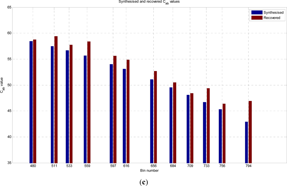
In this paper, we have developed and applied MCMC and RJMCMC simulation algorithms for Bayesian inference of the structural and biochemical parameters of a tree or forest canopy from multispectral LiDAR data. In particular, using a heterogeneous layered model, we have shown how it is possible to recover area indices as a function of variable “layer” position from a single LiDAR waveform, allowing a more detailed model of the structural profile than the commonly applied measures discussed in our review. We then extended our analysis to infer both structural and photochemical properties using a part-simulated set of four spectral LiDAR signatures.

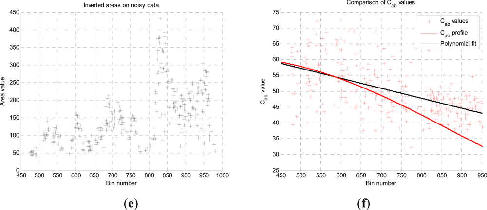
This analysis showed that is possible to combine the structural and photochemical inversion in a two-stage process, but that the problem is not fully resolved for several parameters. Constraining the analysis to a single parameter of interest, we were able to recover the chlorophyll profile as a function of tree or canopy depth, although this showed considerable variance when applied to simulated noisy data. In general, variations in the LiDAR spectra can be caused by tree species, the relative abundance of mixture components, changes in underlying terrain and structure such as slopes, and many other biochemical parameters in addition to chlorophyll content, as included in the PROSPECT model. Our analysis has made a number of a priori assumptions that would need to be justified in any deployed aerial or satellite system. Further, we have been restricted by the availability of suitable multispectral data, which has led to the inclusion of two different datasets for analysis, none of which is wholly satisfactory.

The work has posed several imperatives for future work. First, the ill-posed nature of the inversion problem suggests we need to deploy a true multispectral or hyperspectral sensor to collect full waveform LiDAR data from natural forest canopies. To fully evaluate such data, we need to perform accompanying, traditional field based methods, e.g., hypsometer height measurements, high resolution, colour digital hemispherical photographs (separating leafy and woody canopy components), and profile radiometric measurements. Second, we need to develop and validate the multi-layer model against this true data, and determine whether this approach is valid for future development. For example, we make no allowance for absorption and transmission, and for the effects of multiple reflections beyond the first return along each ray direction. Third, we need to progressively remove some of the a priori assumptions that we make when interpreting the data. Finally, although we are enthused by the prospect of hyperspectral LiDAR, we would not rule out the benefits of simultaneous recovery of passive hyperspectral imagery which may make interpretation of multispectral LiDAR data better posed.

An extension of the ground based and simulation work presented here will take steps towards resolving forest structure and processes directly related to vegetation productivity. However there is a real need for an active (laser) system capable of measuring both structural parameters and physiological changes throughout entire forested canopies, including the understorey, which is only achievable from an airborne or spaceborne platform. At the time of writing no dedicated capability exists to increase the capacity for mapping biomass carbon and measure dynamic topography and ecosystem change in great detail. The proposed BIOMASS (European Space Agency) Earth Explorer mission is an attempt to address this issue, albeit with a capacity to monitor dramatic changes and re-growth, rather than detailed forest parameters at a high resolution directly. In this regard, an airborne or spaceborne multi spectral lidar instrument would provide valuable complementary data with greater information content, but less spatial coverage. This would be further enhanced by the capacity for vertically resolved discrimination of the types of surfaces that can be separated by spectral characteristics. A LiDAR instrument that actively measures vegetation spectral response in well-chosen narrow wavelength bands would provide unprecedented information both as a detailed sampling tool and for calibration of passively acquired multi-spectral vegetation data.