Artificial Neural Network Approach for Mapping Contrasting Tillage Practices

Abstract

Tillage information is crucial for environmental modeling as it directly affects evapotranspiration, infiltration, runoff, carbon sequestration, and soil losses due to wind and water erosion from agricultural fields. However, collecting this information can be time consuming and costly. Remote sensing approaches are promising for rapid collection of tillage information on individual fields over large areas. Numerous regression-based models are available to derive tillage information from remote sensing data. However, these models require information about the complex nature of underlying watershed characteristics and processes. Unlike regression-based models, Artificial Neural Network (ANN) provides an efficient alternative to map complex nonlinear relationships between an input and output datasets without requiring a detailed knowledge of underlying physical relationships. Limited or no information currently exist quantifying ability of ANN models to identify contrasting tillage practices from remote sensing data. In this study, a set of Landsat TM-based ANN models was developed to identify contrasting tillage practices in the Texas High Plains. Observed tillage data from Moore and Ochiltree Counties were used to develop and evaluate the models, respectively. The overall classification accuracy for the 15 models developed with the Moore County dataset varied from 74% to 91%. Statistical evaluation of these models against the Ochiltree County dataset produced results with an overall classification accuracy varied from 66% to 80%. The ANN models based on TM band 5 or indices of TM Band 5 may provide consistent and accurate tillage information when applied to the Texas High Plains.

1. Introduction

Knowledge on prevailing adoption rate of conservation tillage practices in relation to topography within a watershed is important for targeting critical areas to reduce soil erosion. It is also helpful to evaluate the success of soil conservation programs that promote adoption of conservation tillage practices. Conservation tillage includes no-till, ridge-till, strip-till, mulch-till and reduced till. Collecting tillage information manually on individual fields at a regional scale can be time consuming, labor intensive, and costly. Moreover, tillage data from few fields in a watershed provide limited capabilities for environmental assessment as they provide point rather than area-based information. Remote sensing techniques promise considerable improvements in providing such spatial data over a large area in a time and cost-effective manner. Conventional methods of mapping tillage practices over a large area include field survey and manual interpretation of film products derived from sensors mounted on aerial or satellite platforms. In a 5-year study, DeGloria et al. [1] manually interpreted the Landsat Multi-Spectral Scanner (MSS) data for identifying land under conventional and conservation tillage practices in the central coastal region of California. They achieved an overall classification accuracy of 81%. Motsch et al. [2] derived a crop residue map showing four tillage categories from Landsat Thematic Mapper (TM) data for Seneca County in northern Ohio with an accuracy of 68%. However, accuracy of their maps was a function of a human interpreter’s ability to identify tillage patterns on the image.

In recent years, numerous regression-based spectral models have been developed to measure crop residue cover or identify contrasting tillage practices [3,4,5,6,7]. These models were based on the differences in the magnitude of spectral responses in visible and near infrared wavelengths for different residue covers. Daughtry et al. [8] evaluated numerous spectral models for estimating crop residue cover using Landsat TM data. They found weak relationships between Landsat TM indices and percentage crop residue cover. Similar results were reported in Minnesota [4]. However, these studies reported higher prediction accuracy when crop residue cover was broadly classified into two categories, (>30% and <30% of residue cover) indicating that Landsat TM indices are useful in identifying contrasting tillage practices.

Linear logistic regression modeling is the most common approach used for mapping tillage practices. A number of studies [9,10,11] have successfully used this technique to develop remote sensing based models for classifying contrasting tillage practices at a regional scale and reported varying degree of accuracy. However, these models should be thoroughly evaluated before using them in different geographic regions to adjust the cut-point probability values in order to attain acceptable classification accuracy or new models may need to be developed when existing models are insensitive to tillage classes [7]. Yet another concern in using logistic regression method for mapping the tillage is that the available data is forced to conform to a predefined model form. Note that the relationship between the sensor data and tillage features is highly nonlinear and unknown. Forcing data to confirm to a predefined model may result in prediction errors. Consequently, most of the regression-based models currently in use often fail to accurately capture this relationship. In this context, data-driven models may be preferable to discover relationships from input-output data even when the user does not have a complete physical understanding of the underlying processes.

The objective of this study was to develop and evaluate Artificial Neural Network (ANN) models to identify contrasting tillage practices in the Texas High Plains. Development of these models is expected to provide a rapid and cost effective approach for mapping contrasting tillage practices over a large agricultural region.

2. Artificial Neural Network (ANN)

An ANN is a nonlinear mathematical structure capable of representing arbitrarily complex nonlinear processes. It can be used to relate inputs and outputs of any system [12]. ANN models have been used successfully to model complex nonlinear input/output time-series relationships in a wide variety of fields including finance [13], medicine [14], physics [15], engineering, geology, and hydrology [16,17]. The main advantage of this approach over traditional methods is that it does not require information on complex processes under consideration to be explicitly described in a mathematical form.

ANNs can be characterized as massive parallel interconnections of simple neurons that function as a collective system. The network topology an ANN consists of a set of nodes (neurons) connected by links and usually organized in a number of layers. Each node in a layer receives and processes the weighted input from a previous layer and transmits its output to nodes in the following layer through links. Each link is assigned a weight, which is a numerical estimate of the connection strength. The weighted summation of inputs to a node is converted to an output according to a transfer function (typically a sigmoid function). Most ANNs have three or more layers: an input layer, which is used to present data to the network; an output layer, which is used to produce an appropriate response to the given input; and one or more intermediate or hidden layers, which are used to act as a collection of feature detectors. Determination of appropriate network architecture is one of the most important, but also one of the most difficult tasks in the model-building process. Unless carefully designed, an ANN model can lead to over parameterization and result in an unnecessarily complex network.

An ANN model of a physical system can be considered as a form of highly complex and nonlinear regression model of undefined structure. For instance, consider an ANN model with n input neurons (x₁, …, x_n), h hidden neurons (z₁, …, z_h), and m output neurons (y₁, …, y_m). Let i, j, and k be the indices representing input, hidden, and output layers, respectively. Let ${\tau }_j$ be the bias for neuron z_j and φ_κ be the bias for neuron y_k. Let w_ij be the weight of the connection from neuron x_i to neuron z_j and β_jκ be the weight of connection from neuron z_j to y_k. The function that an ANN calculates is:

$$y_k=g_A\left({\displaystyle \sum _{j=1}^h{z}_j{\beta }_{jk}+{\varphi }_k}\right)$$

(1)

$$z_j=f_A\left({\displaystyle \sum _{i=1}^n{x}_i{w}_{ij}+{\tau }_j}\right)$$

(2)

where g_A and f_A are activation functions, which are usually continuous, bounded, and non-decreasing. The usual choice is the logistic function for a variable s is defined as:

$$f(s)\hspace{0.17em}\hspace{0.17em}\hspace{0.17em}\text{or}\hspace{0.17em}\hspace{0.17em}\hspace{0.17em}g(s)=\frac{1}{1+e^{-s}}$$

(3)

The training of an ANN involves finding the optimal weight vector for the network. Many training techniques are available. The aim of network training is to find a global solution to the weight matrix, which is typically a nonlinear optimization problem [18]. Consequently, the theory of nonlinear optimization is applicable to the training of ANNs. The suitability of a particular method is generally a compromise between computation cost and performance, and the most popular is the back propagation algorithm [19].

3. Study Area and Data

This study was conducted with tillage data collected from 76 commercial operated farms (31 in Moore and 41 in Ochiltree Counties) in the Texas High Plains (Figure 1). Moore County is located in the north-central part of the Texas High Plains and has a total area of 236,826 ha. Two-thirds of the land is in the nearly level, smooth uplands of the High Plains [20] and most of it under row crop production. Corn, sorghum, and wheat are the major crops in the Moore County. In 2004, it ranked 5th in corn production and accounted for about 5.7% of the total corn production in Texas [21]. Ochiltree County is 234,911 ha in area with more than 70% of the land under crop production. Sorghum, wheat and corn are the major crops in the county. In 2004, Ochiltree County ranked 8^th in Texas in sorghum production and accounted for about 2.4% of the state total sorghum production [21]. Typical planting dates for major summer crops in the study area vary anywhere from the 2nd week of April to the 3rd week of May. Annual average precipitation is about 481 and 562 mm for Moore and Ochiltree Counties, respectively. Crop water needs are supplemented with groundwater from the underlying Ogallala Aquifer. Nearly level to gently sloping fields with silty clay soils of the Sherm series occupy nearly the entire crop lands in both Moore and Ochiltree Counties. Conventional tillage practices in these counties usually consist of offset disk in the fall. Common conservation tillage practices are no plowing in the fall, and sweep or disk plowing at planting that leaves at least 30% of the surface covered with crop residue after planting.

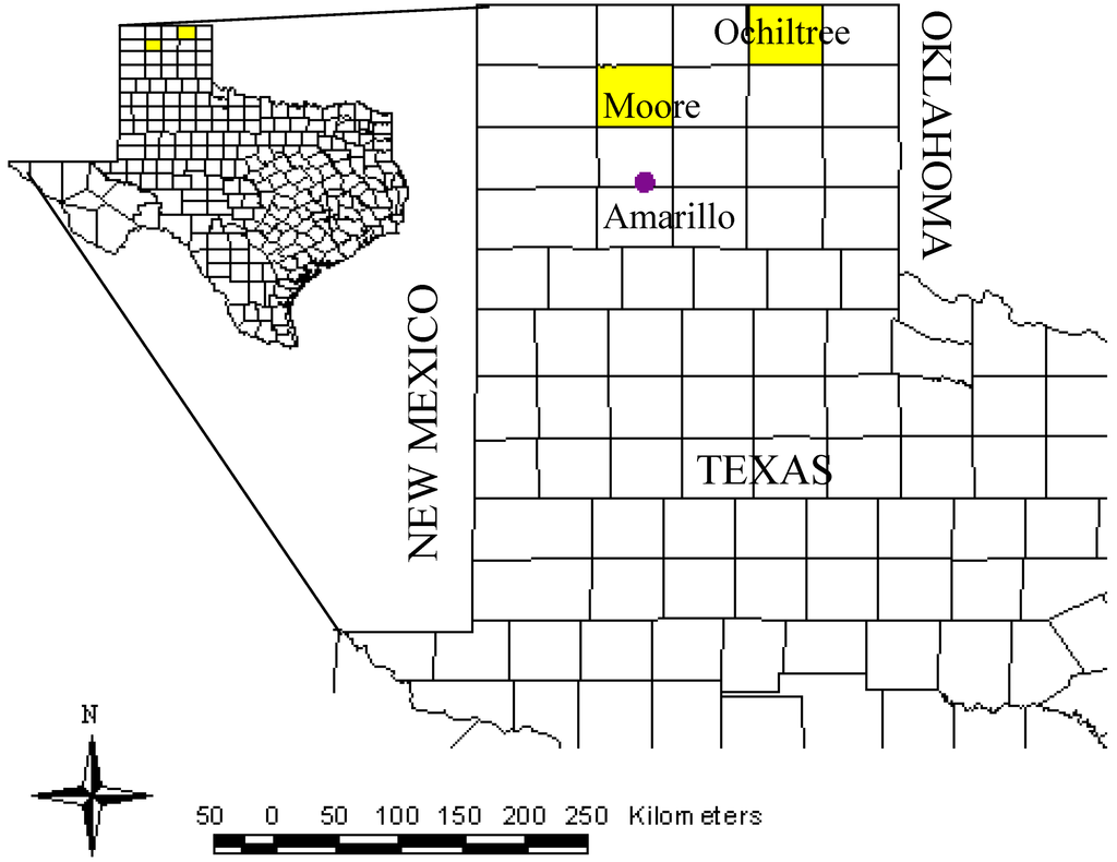
Figure 1. Location of Moore and Ochiltree Counties in the Texas High Plains, USA.

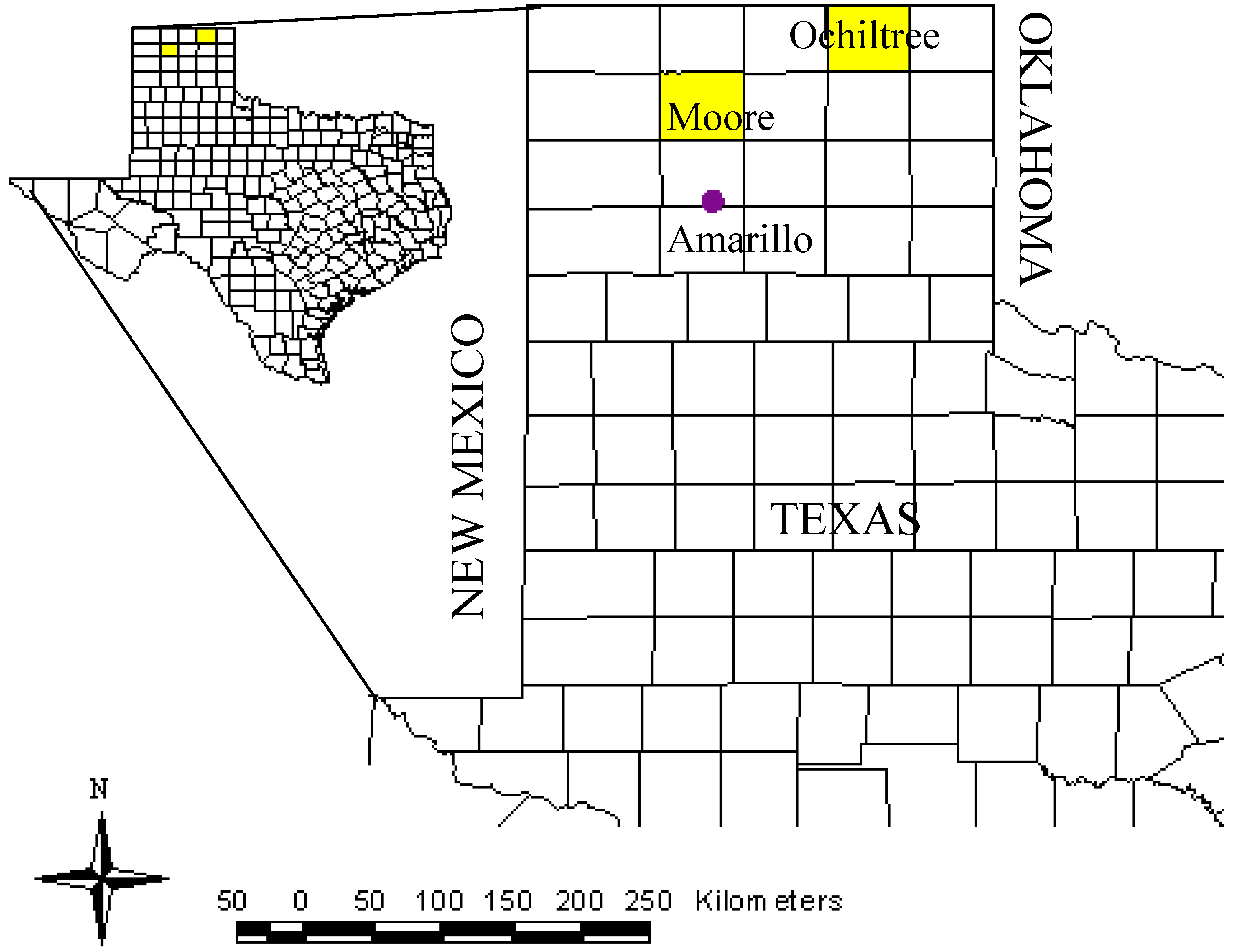
Figure 1. Location of Moore and Ochiltree Counties in the Texas High Plains, USA.

4. Materials and Methods

In this study, the development and evaluation of tillage models consisted of four steps: (1) remote sensing data acquisition, (2) ground-truth data collection, (3) development of ANN models, and (4) evaluation of models using percent correct and kappa (k) statistic. Two, Level-1 processed precision corrected Landsat TM scenes acquired during the 2005 pre-planting season were used for model development and evaluation purposes. One scene was acquired by the satellite on May 10, 2005 for Ochiltree County (Path 30 / Row 35) and the other scene was acquired on May 17, 2005 for Moore County (Path 31 / Row 35). Ground-truth survey of prevailing tillage practices in Moore and Ochiltree Counties were scheduled to coincide with satellite overpass days. Tillage data was collected from 35 and 41 randomly selected commercial fields in Moore and Ochiltree Counties, respectively. Ground-truth data included geographic coordinates obtained using a handheld Global Positioning System (GPS), infrared images of residue cover taken at 2-m height using the Agricultural Digital Camera [Dycam Inc. (Mention of trade or commercial products in this article is solely for the purpose of providing specific information and does not imply recommendation or endorsement by the US Department of Agriculture.), Chatsworth, CA, USA], and digital pictures of residue cover taken with a 5 Mega pixel digital camera.

The crop residue cover was estimated by classifying the infrared images using Multispec© image processing software developed by the Purdue Research Foundation. Tillage practices were assigned a class value of 0 for conventional tillage and 1 for conservation tillage. Tillage classification was based on the percentage of the soil surface covered with crop residue. We defined conservation tillage systems as those that retained at least 30% of the soil surface covered with crop residue after a crop was planted. The tillage and crop residue characteristics of selected commercial fields in Moore and Ochiltree Counties are presented in Table 1.

Table 1. Tillage and crop residue characteristics of randomly selected commercial fields for ground truth data from Moore and Ochiltree Counties, Texas during the 2005 pre-planting season.

Tillage	Number of Fields	Crop Residue
		Corn	Soybean	Sorghum	Wheat	Others
Moore County
Conservation Tillage	19	10	1	3	4	1
Conventional Tillage	16	8	–	3	5	–
Total	35	18	1	6	9	1
Ochiltree County
Conservation Tillage	20	2	0	8	10	–
Conventional Tillage	21	2	7	7	4	1
Total	41	4	7	15	14	1

Table 1. Tillage and crop residue characteristics of randomly selected commercial fields for ground truth data from Moore and Ochiltree Counties, Texas during the 2005 pre-planting season.

Tillage	Number of Fields	Crop Residue
		Corn	Soybean	Sorghum	Wheat	Others
Moore County
Conservation Tillage	19	10	1	3	4	1
Conventional Tillage	16	8	–	3	5	–
Total	35	18	1	6	9	1
Ochiltree County
Conservation Tillage	20	2	0	8	10	–
Conventional Tillage	21	2	7	7	4	1
Total	41	4	7	15	14	1

Table 2. Mean brightness values for each field in Moore and Ochiltree Counties.^†

Tillage Practice & Statistic	TM1	TM2	TM3	TM4	TM5	TM6	TM7
Moore County
Conservation Tillage
Mean	105.2	53.8	71.9	81.6	157.3	132.2	85.6
Standard Deviation	10.2	5.3	6.4	7.5	13.2	13.3	6.1
Conventional Tillage
Mean	97.8	48.5	63.3	73.3	132.1	131.6	75.3
Standard Deviation	8.3	3.7	5.5	6.7	15.9	11.9	8.8
Ochiltree County
Conservation Tillage
Mean	102.2	53.3	73.7	82.6	181.2	162.4	110.9
Standard Deviation	5.9	4.6	7.2	8.7	13.9	2.1	16.0
Conventional Tillage
Mean	93.7	47.7	64.4	72.2	157.2	162.0	99.7
Standard Deviation	8.9	5.8	8.9	9.7	17.8	3.4	11.6

^† TM1, TM2, etc. are TM bands 1, 2, etc.

Table 2. Mean brightness values for each field in Moore and Ochiltree Counties.^†

Tillage Practice & Statistic	TM1	TM2	TM3	TM4	TM5	TM6	TM7
Moore County
Conservation Tillage
Mean	105.2	53.8	71.9	81.6	157.3	132.2	85.6
Standard Deviation	10.2	5.3	6.4	7.5	13.2	13.3	6.1
Conventional Tillage
Mean	97.8	48.5	63.3	73.3	132.1	131.6	75.3
Standard Deviation	8.3	3.7	5.5	6.7	15.9	11.9	8.8
Ochiltree County
Conservation Tillage
Mean	102.2	53.3	73.7	82.6	181.2	162.4	110.9
Standard Deviation	5.9	4.6	7.2	8.7	13.9	2.1	16.0
Conventional Tillage
Mean	93.7	47.7	64.4	72.2	157.2	162.0	99.7
Standard Deviation	8.9	5.8	8.9	9.7	17.8	3.4	11.6

^† TM1, TM2, etc. are TM bands 1, 2, etc.

Ground truth locations on each image were identified using the GPS coordinates for extracting spectral reflectance data from each TM band image. In Landsat TM data, reflectance values are stored as brightness values (or digital numbers) in the 8-bit format. The raw brightness values for ground truth pixels were extracted and analyzed using image processing software. Table 2 presents the mean brightness values for Moore and Ochiltree Counties. For model development and evaluation, mean reflectance data from 9-pixels (ground-truth pixel and surrounding 8 pixels) was used. The Moore County dataset was used for model development and the Ochiltree County dataset was used for model testing.

For ANN model development, TM indices were developed with all possible combinations of two bands from all seven Landsat 5 TM bands. The TM indices included difference indices, sum indices, product indices, ratio indices, and normalized difference indices. ANN models were developed to derive tillage information with inputs as (1) the brightness value for each TM band and various combinations, and (2) each difference, sum, product, and normalized difference index. Sigmoid function was used in the hidden and output layers of the ANN. The number of hidden nodes in the hidden layer was identified by trial and error, as currently there is no guideline to derive number of hidden layers a priory. The back propagation method was used for optimization of the ANN models. Since the output of an ANN was a tillage probability value between 0 and 1, a cut point tillage probability that yields the highest percent correct for each model was suggested for tillage classification. Considering the performance of the models in terms of percent correct, a set of best models was selected for validation with Ochiltree County dataset.

The selected models were evaluated against the Ochiltree County dataset for their ability to accurately identify conservation and conventional tillage systems. Two methods were used to determine tillage classification accuracy. In Method I, cut-point probabilities derived from the Moore County dataset were used, whereas in Method II, cut-point probabilities were determined by comparing ground-truth data with tillage probability values to maximize the tillage classification accuracy.

For model selection and evaluation, error matrices [22] were developed for selected ANN models to determine the overall classification accuracy (percent correct) and kappa (k) values. Percent correct was calculated by dividing the sum of correctly classified fields by the total number of fields examined. The “k value is a measure of the difference between two maps and the agreement that might be contributed solely by chance matching of the two maps” [23]. The k value was calculated as:

$$k=\frac{Observed-Expected}{1-Expected}$$

(4)

where “observed” is the percent correct and “expected” is an estimate of the chance agreement to the “observed.” A k value of +1.0 indicates perfect accuracy of the classification. Models with a k value of 0.4 or more is considered good.

5. Results and Discussion

Table 1 presents ground-truth data collected in the Moore and Ochiltree Counties, respectively, during 2005 planting season. Moore County dataset consisted of 19 fields in conservation tillage and 16 fields in conventional tillage. About 53% of the conservation and 50% of conventionally tilled fields had corn residue. Sorghum residue was found in 3 fields in each tillage category and 5 out of 9 fields with wheat residue were conventionally tilled. The mean soil organic carbon and soil water content were 1.39% and 0.22 m³ m⁻³, respectively, in conventionally tilled fields. Out of 41 fields in Ochiltree County, conservation tillage was found in 20 fields and about 50% of these fields had wheat residue. Conventional tillage was found in 21 fields, and only 19% of these had wheat residue. About 40% of the conservation and 33% of conventionally tilled fields had sorghum residue. Soybean fields accounted for 33% of the conventionally tilled fields and none under conservation tillage. Fields with conservation tillage generally exhibited greater mean brightness values than did conventionally tilled fields (Table 2). This is consistent with results reported by van Deventer et al. [9] and Stoner et al. [24], but contrary to Bricklemyer et al. [11], who found that conventionally tilled fields exhibited greater brightness values than did conservation tillage in Montana.

Table 3. Landsat TM based ANN models’ performance for mapping tillage practices in Moore County, Texas.

Model Inputs†	Hidden Nodes	Cut Point (%)	Correct Predictions (%)
			All Fields	Conservation Tillage	Conventional Tillage
TM4 & TM5	5	47	91	95	90
R45 & R46	5	49	91	95	90
NDTI15 & NDTI56	6	59	89	85	95
TM5 & TM6	4	58	89	85	95
R35 & R36	5	50	89	90	90
TM5 & TM7	5	51	89	95	86
D15 & D16	5	43	89	95	86
TM2, TM4, TM5 & TM6	5	48	86	95	81
TM2 & TM5	5	50	83	90	81
TM3 & TM5	5	49	83	90	81
TM1 & TM5	5	40	83	95	76
TM4 & TM7	5	53	74	80	76
TM1 & TM4	5	48	74	80	76
TM4, TM5, & TM6	5	50	69	75	71
TM4 & TM6	5	50	66	75	67

^† TM1, TM2, etc. are TM bands 1, 2, etc.; NDTI − Normalized Difference Tillage Index; R45 = TM4/TM5; R46 = TM4/TM6; R35 = TM3/TM5; R36 = TM3/TM6; D15 = TM1 − TM5; D16 = TM1 − TM6; NDTI15 = (TM1 − TM5)/(TM1 + TM5); NDTI56 = (TM5 − TM6)/(TM5+TM6).

Table 3. Landsat TM based ANN models’ performance for mapping tillage practices in Moore County, Texas.

Model Inputs†	Hidden Nodes	Cut Point (%)	Correct Predictions (%)
			All Fields	Conservation Tillage	Conventional Tillage
TM4 & TM5	5	47	91	95	90
R45 & R46	5	49	91	95	90
NDTI15 & NDTI56	6	59	89	85	95
TM5 & TM6	4	58	89	85	95
R35 & R36	5	50	89	90	90
TM5 & TM7	5	51	89	95	86
D15 & D16	5	43	89	95	86
TM2, TM4, TM5 & TM6	5	48	86	95	81
TM2 & TM5	5	50	83	90	81
TM3 & TM5	5	49	83	90	81
TM1 & TM5	5	40	83	95	76
TM4 & TM7	5	53	74	80	76
TM1 & TM4	5	48	74	80	76
TM4, TM5, & TM6	5	50	69	75	71
TM4 & TM6	5	50	66	75	67

^† TM1, TM2, etc. are TM bands 1, 2, etc.; NDTI − Normalized Difference Tillage Index; R45 = TM4/TM5; R46 = TM4/TM6; R35 = TM3/TM5; R36 = TM3/TM6; D15 = TM1 − TM5; D16 = TM1 − TM6; NDTI15 = (TM1 − TM5)/(TM1 + TM5); NDTI56 = (TM5 − TM6)/(TM5+TM6).

The performances of the 15 best ANN models in identifying the tillage practices in Moore County are presented in Table 3. It is noted that the cut-point probabilities that yielded higher classification accuracy were varied from 0.43 to 0.59 and were close to the theoretical cut-point probability of 0.5. Models with combinations of TM band 4, 5 and/or 6 were shown to be useful for tillage identification purposes, with the best results obtained with the model that used TM bands 4 and 5. This model accurately classified 32 (91%) out of the 35 fields sampled in Moore County with a k value of 0.83. This indicates that reflectance values in the mid-infrared spectral range (1.55–1.75 µm) are highly sensitive to crop residue, and generally show higher reflectance in conservation tillage fields than in conventionally tilled fields (Table 2).

With the validation dataset from Ochiltree County, it was observed that the performance of an ANN model that used TM band 4 and 5 information predicted 71% of the fields accurately with a k value of 0.42, when Method-I was used for evaluation (Table 4). The poor performance can be attributed to differences in TM band 5 brightness values between Moore and Ochiltree Counties. The mean brightness value for conservation tillage in Moore County was about 3% greater than that for the Ochiltree County (Table 2). Similar variation was found for conventional tillage. The model that used NDTI15 (normalized difference between TM bands 1 and 5) and NDTI56 (normalized difference between TM bands 5 and 6) as inputs showed similar performance during both training (Moore County) and validation (Ochiltree County).

Table 4. Validation performance of Landsat 5 TM based ANN models used for mapping tillage practices in Ochiltree County, Texas using Method-I (Cutoff probabilities values derived from the training data i.e., Moore County data).

Model Inputs†	Cut Point (%)	Kappa	Correct Predictions (%)
			All Fields	Conservation Tillage	Conventional Tillage
TM4 & TM5	47	0.42	71	74	56
TM5 & TM7	51	0.47	73	95	38
TM2 & TM5	50	0.42	71	89	38
TM3 & TM5	49	0.42	71	84	44
TM4, TM5 & TM6	50	0.42	71	89	38
D15 & D16	43	0.47	73	95	38
NDTI15 & NDTI56	59	0.56	78	79	69
TM5 & TM6	58	0.46	73	74	63
R35 & R36	50	0.47	73	95	38
R45 & R46	49	0.47	73	89	44
TM1 & TM5	40	0.47	73	95	38
TM4 & TM7	53	0.42	71	74	56
TM2, TM4, TM5, & TM6	48	0.41	71	68	63
TM4 & TM6	50	0.32	66	89	25
TM1 & TM4	48	0.37	68	79	44

^† TM1, TM2, etc. are TM bands 1, 2, etc.; R45 = TM4/TM5; R46 = TM4/TM6; R35 = TM3/TM5; R36 = TM3/TM6; D15 = TM1 − TM5; D16 = TM1 − TM6; NDTI15 = (TM1 − TM5)/(TM1 + TM5); NDTI56 = (TM5 − TM6)/(TM5 + TM6).

Table 4. Validation performance of Landsat 5 TM based ANN models used for mapping tillage practices in Ochiltree County, Texas using Method-I (Cutoff probabilities values derived from the training data i.e., Moore County data).

Model Inputs†	Cut Point (%)	Kappa	Correct Predictions (%)
			All Fields	Conservation Tillage	Conventional Tillage
TM4 & TM5	47	0.42	71	74	56
TM5 & TM7	51	0.47	73	95	38
TM2 & TM5	50	0.42	71	89	38
TM3 & TM5	49	0.42	71	84	44
TM4, TM5 & TM6	50	0.42	71	89	38
D15 & D16	43	0.47	73	95	38
NDTI15 & NDTI56	59	0.56	78	79	69
TM5 & TM6	58	0.46	73	74	63
R35 & R36	50	0.47	73	95	38
R45 & R46	49	0.47	73	89	44
TM1 & TM5	40	0.47	73	95	38
TM4 & TM7	53	0.42	71	74	56
TM2, TM4, TM5, & TM6	48	0.41	71	68	63
TM4 & TM6	50	0.32	66	89	25
TM1 & TM4	48	0.37	68	79	44

^† TM1, TM2, etc. are TM bands 1, 2, etc.; R45 = TM4/TM5; R46 = TM4/TM6; R35 = TM3/TM5; R36 = TM3/TM6; D15 = TM1 − TM5; D16 = TM1 − TM6; NDTI15 = (TM1 − TM5)/(TM1 + TM5); NDTI56 = (TM5 − TM6)/(TM5 + TM6).

Table 5 presents a set of ANN models that performed well when Method-II was used with the Ochiltree dataset. It is noted that conservation tillage was predicted with relatively greater accuracy by most of the models. It is also noted that the model that used NDTI15 and NDTI56 as inputs had the same cut point for classification for training and validation (0.59 for both Moore County as well as Ochiltree County) indicating the robustness of the generalization properties. The validation of the model using an independent data set from a different county suggests that this model (NDTI15 and NDTI56 as inputs) may be useful to derive tillage information in the Texas High Plains region. These results confirmed that models that contained TM bands 5 and 6 or indices that contain TM bands 5 and 6 are highly sensitive to crop residue surface. This is consistent with results reported in van Deventer et al. [9] and Bricklemyer et al. [11].

Table 5. Validation performance of Landsat 5 TM based ANN models used for mapping tillage practices in Ochiltree County, Texas using Method-II (Cutoff probabilities values associated with maximum percent correct in the validation data).

Model Inputs†	Cut Point (%)	Kappa	Correct Predictions (%)
			All Fields	Conservation Tillage	Conventional Tillage
TM4 & TM5	38	0.47	73	95	38
TM5 & TM7	51	0.47	73	95	38
TM2 & TM5	50	0.42	71	89	38
TM3 & TM5	48	0.42	71	89	38
TM4, TM5 & TM6	50	0.42	71	89	38
D15 & D16	43	0.47	73	95	38
NDTI15 & NDTI56	59	0.56	78	79	69
TM5 & TM6	58	0.46	73	74	63
R35 & R36	68	0.51	76	79	63
R45 & R46	73	0.56	78	84	63
TM1 & TM5	40	0.47	73	95	38
TM4 & TM7	53	0.42	71	74	56
TM2, TM4, TM5, & TM6	48	0.41	71	68	63
TM4 & TM6	50	0.32	66	89	25
TM1 & TM4	42	0.48	71	84	44

^† TM1, TM2, etc. are TM bands 1, 2, etc; R45 = TM4/TM5; R46 = TM4/TM6; R35 = TM3/TM5; R36 = TM3/TM6; D15 = TM1 − TM5; D16 = TM1 − TM6; NDTI15 = (TM1 − TM5)/(TM1 + TM5); NDTI56 = (TM5 − TM6)/(TM5 + TM6).

Table 5. Validation performance of Landsat 5 TM based ANN models used for mapping tillage practices in Ochiltree County, Texas using Method-II (Cutoff probabilities values associated with maximum percent correct in the validation data).

Model Inputs†	Cut Point (%)	Kappa	Correct Predictions (%)
			All Fields	Conservation Tillage	Conventional Tillage
TM4 & TM5	38	0.47	73	95	38
TM5 & TM7	51	0.47	73	95	38
TM2 & TM5	50	0.42	71	89	38
TM3 & TM5	48	0.42	71	89	38
TM4, TM5 & TM6	50	0.42	71	89	38
D15 & D16	43	0.47	73	95	38
NDTI15 & NDTI56	59	0.56	78	79	69
TM5 & TM6	58	0.46	73	74	63
R35 & R36	68	0.51	76	79	63
R45 & R46	73	0.56	78	84	63
TM1 & TM5	40	0.47	73	95	38
TM4 & TM7	53	0.42	71	74	56
TM2, TM4, TM5, & TM6	48	0.41	71	68	63
TM4 & TM6	50	0.32	66	89	25
TM1 & TM4	42	0.48	71	84	44

^† TM1, TM2, etc. are TM bands 1, 2, etc; R45 = TM4/TM5; R46 = TM4/TM6; R35 = TM3/TM5; R36 = TM3/TM6; D15 = TM1 − TM5; D16 = TM1 − TM6; NDTI15 = (TM1 − TM5)/(TM1 + TM5); NDTI56 = (TM5 − TM6)/(TM5 + TM6).

6. Summary

Availability of accurate information on prevailing tillage practices will aid in the assessment and adoption of appropriate tillage practices to reduce soil erosion and nutrient losses. A set of Landsat 5 TM-based ANN models was developed and evaluated for identifying contrasting tillage practices in the Texas High Plains. Overall classification accuracy of the 15 models developed with the Moore County dataset varied from 74% to 91%. Evaluation of these models against an independent dataset from Ochiltree County produced somewhat poorer but still acceptable results with an overall classification accuracy varied from 66% to 80%. These validation results indicate that region-specific cut points may be needed to maintain or improve the accuracy of the tillage models. Further evaluation of these models in different geographic regions is needed to evaluate their regional robustness to identify contrasting tillage practices. ANN models found to be easy to develop, cost and time effective, and produced reasonably accurate tillage classification results. This approach is promising for the rapid collection of tillage information on individual fields over large areas.

References

- DeGloria, S.D.; Wall, S.L.; Benson, A.S.; Whiting, M.L. Monitoring conservation tillage practices using Landsat multispectral data. J. Soil Water Conserv. 1986, 41, 187–189. [Google Scholar]
- Motsch, B.; Schaal, G.; Lyon, J.G.; Logan, T.J. Monitoring crop residue in Senaca County, Ohio. In Proceedings of the ASPRS Meeting, Cleveland, OH, USA, 1990; pp. 66–76.
- Sullivan, D.G.; Shaw, J.N.; Mask, P.; Rickman, D.; Luvall, J.; Wersinger, J.M. Evaluation of multispectral data for rapid assessment of in situ wheat straw residue cover. Soil Sci. Soc. Amer. J. 2004, 68, 2007–2013. [Google Scholar] [CrossRef]
- Thoma, D.P.; Gupta, S.C.; Bauer, M.E. Evaluation of optical remote sensing models for crop residue cover assessment. J. Soil Water Conserv. 2004, 59, 224–233. [Google Scholar]
- Daughtry, C.S.T.; Hunt, E.R., Jr.; Doraiswamy, P.C.; McMurtrey, J.M., III. Remote sensing the spatial distribution of crop residues. Agron. J. 2005, 97, 864–878. [Google Scholar] [CrossRef]
- Sullivan, D.G.; Truman, C.C.; Schomberg, H.H.; Endale, D.M.; Strickland, T.C. Evaluating techniques for determining tillage regime in the Southeastern Coastal Plain and Piedmont. Agron. J. 2006, 98, 1236–1246. [Google Scholar] [CrossRef]
- Gowda, P.H.; Howell, T.A.; Evett, S.R.; Chavez, J.L.; New, L. Remote sensing of contrasting tillage practices in the Texas Panhandle. Int. J. Remote Sens. 2008, 29, 3477–3487. [Google Scholar] [CrossRef]
- Daughtry, C.S.T.; Doraiswamy, P.C.; Hunt, E.R., Jr.; Stern, A.J.; McMurtrey, J.E.; Prueger, J.H. Remote sensing of crop residue cover and soil tillage intensity. Soil Till. Res. 2006, 91, 101–108. [Google Scholar] [CrossRef]
- van Deventer, A.P.; Ward, A.D.; Gowda, P.H.; Lyon, J.G. Using Thematic Mapper data to identify contrasting soil plains and tillage practices. Photogramm. Eng. Remote Sening 1997, 63, 87–93. [Google Scholar]
- Vina, A.; Peters, A.J.; Ji, L. Use of multispectral Ikonos imagery for discriminating between conventional and conservation agricultural tillage practices. Photogramm. Eng. Remote Sens. 2003, 69, 537–544. [Google Scholar] [CrossRef]
- Bricklemyer, R.S.; Lawrence, R.L.; Miller, P.R.; Battogtokh, N. Predicting tillage practices and agricultural soil disturbance in north-central Montana with Landsat imagery. Agr. Ecosyst. Environ. 2006, 114, 210–216. [Google Scholar] [CrossRef]
- Hornik, K.; Stinchcombe, M.; White, H. Multilayer feed forward network are universal approximators. Neural Networks 1989, 2, 359–366. [Google Scholar] [CrossRef]
- Buscema, M.; Sacco, P.L. Feedforward networks in financial predictions: the future that modifies the present. Expert Syst. 2000, 17, 149–169. [Google Scholar]
- DeRoach, J.N. Neural networks: an artificial intelligence approach to the analysis of clinical data. Aust. Phys. Eng. Sci. Med. 1989, 12, 100–106. [Google Scholar]
- Gernoth, K.A.; Clark, J.W.; Prater, J.S.; Bohr, H. Neural network models of nuclear systematics. Phys. Lett. Bull. 1993, 300, 1–7. [Google Scholar] [CrossRef]
- ASCE Task Committee on Application of Artificial Neural Networks in Hydrology. Artificial neural networks in hydrology I: Preliminary concepts. J. Hydrol. Eng. ASCE 2000, 5, 115–123.
- ASCE Task Committee on Application of Artificial Neural Networks in Hydrology. Artificial neural networks in hydrology II: Hydrologic applications. J. Hydrol. Eng. ASCE 2000, 5, 124–137.
- White, H. Learning in artificial neural networks: a statistical perspective. Neural Comp. 1989, 1, 425–464. [Google Scholar] [CrossRef]
- Rumelhart, D.E.; Hinton, D.E.; Williams, R.J. Learning Internal Representations by Error Propagation. In Parallel Distributed Processing: Explorations in the Microstructure of Cognition; Rumelhart, D.E., Mc-Clelland, J.L., Eds.; MIT Press: Cambridge, MA, USA, 1986; pp. 318–364. [Google Scholar]
- USDA-SCS. Soil Survey of Moore County, Texas; Soil Conservation Service, US Department of Agriculture: Washington, DC, USA, 1975; p. 57.
- NASS. 2004 Texas Agricultural Statistics: Texas Agriculture by the Numbers; Bulletin 263; National Agricultural Statistics Service, US Department of Agriculture: Austin, TX, USA, 2005.
- Campbell, J.B. Introduction to Remote Sensing; Guilford Press: New York, NY, USA, 1987. [Google Scholar]
- Congalton, R.G.; Green, K. Assessing the Accuracy of Remotely Sensed Data: Principles and Practices; CRC Press LLC: Boca Raton, FL, USA, 1999; p. 132. [Google Scholar]
- Stoner, E.R.; Baumgartner, M.F.; Weismiller, R.A.; Biehl, L.L.; Robinson, B.F. Extension of laboratory measured soil spectra to field conditions. Soil Sci. Soc. Amer. J. 1980, 44, 572–574. [Google Scholar] [CrossRef]
© 2010 by the authors; licensee Molecular Diversity Preservation International, Basel, Switzerland. This article is an open-access article distributed under the terms and conditions of the Creative Commons Attribution license (http://creativecommons.org/licenses/by/3.0/).