Sea Ice and Water Segmentation in SAR Imagery Based on Polarization Channel Interaction and Edge Selective Fusion

Highlights

What are the main findings?

• A Polarization-Fused Edge-Enhanced framework (PFEE-UNet) is developed for high-resolution SAR sea ice segmentation.
• Cross-Polarization Channel Interaction and Selective Edge Fusion effectively enhance ice–water discrimination and boundary continuity in complex environments.

What are the implications of the main findings?

• The polarization channels’ interaction enhances the representation of SAR features for complex ice–water structure and the model’s response to semantically significant regions, indicating the importance of sufficient fusion of polarizations.
• The proposed method demonstrates robust performance on the AI4Arctic/ASIP dataset and real Sentinel-1 SAR scenes, supporting operational sea ice monitoring and navigation safety.

Abstract

Sea ice segmentation based on Synthetic Aperture Radar (SAR) images has become an important technical means for polar climate change monitoring and navigation safety guarantee. However, the existing methods have limitations in the utilization of SAR polarization information and the modeling of local diversity details of sea ice, which leads to insufficient segmentation, especially in complex ice-water boundary regions. To address these issues, this paper proposes a novel Polarization-Fused Edge-Enhanced UNet (PFEE-UNet) designed specifically for sea ice segmentation from high-resolution SAR images. Specifically, we design the Cross-Polarization Channel Interaction (CPCI) module, which employs a dual interaction strategy of hierarchical inter-group cascading and symmetric cross-fusion. This approach effectively leverages the complementary features of the HH and HV polarization channels, significantly enhancing the distinction between sea ice and open water. Additionally, we present the Dense–Sparse Diversity Enhancement (DSDE) module, which combines a spatial-channel joint attention mechanism to strengthen the model’s ability to capture spatial relationships within complex ice–water structures, effectively alleviating misclassifications caused by abrupt local texture changes. Finally, we design the Selective Edge Fusion (SEF) module, which dynamically selects and integrates multi-level edge features, improving the continuity of sea ice boundaries and preserving its morphological integrity. The experimental results show that the proposed PFEE-UNet model outperforms mainstream segmentation methods on the AI4Arctic/ASIP sea ice dataset, achieving an average Intersection over Union (IoU) of 84.48%, which surpasses existing methods such as HRNet (82.52%) and DeepLabv3+ (82.40%). Additionally, PFEE-UNet was applied for end-to-end ice–water segmentation on real-world Sentinel-1 SAR scenes, demonstrating its effectiveness and robustness for practical sea ice monitoring.

1. Introduction

In the polar climate system, sea ice plays a critical role in regulating heat, gas, and momentum exchanges between the ocean and the atmosphere, as well as influencing surface albedo, thus having profound impacts on both regional and global climate change [1]. At the same time, sea ice provides essential habitats for polar ecosystems and helps maintain ice shelf stability by attenuating ocean wave energy [2]. With the increasing frequency of Arctic shipping and scientific expeditions, the need to rapidly and accurately obtain sea ice distribution information has become crucial for ensuring navigational safety and supporting climate research [3,4]. To achieve continuous monitoring of sea ice distribution and evolution, remote sensing technology has become the most important monitoring tool. Thanks to its advantages of continuous and efficient observation, remote sensing data are widely applied in studies of sea ice type identification, concentration inversion, and boundary detection. Among these, Synthetic Aperture Radar (SAR), with its all-weather, all-time, and wide-area imaging capabilities [5], has become one of the core data sources for sea ice monitoring in polar regions [6].

In recent years, extensive efforts have been devoted to sea ice/ocean segmentation and the identification of leads and polynyas, with methodological paradigms evolving from threshold-based discrimination and statistical inference to machine learning and deep neural modeling [7,8]. Early approaches primarily relied on intensity thresholding and probabilistic modeling to distinguish sea ice from open water. Histogram-based thresholding after speckle filtering [9] and incidence-angle-normalized backscatter correction were commonly adopted to reduce radiometric inconsistency in SAR observations. However, open-water backscatter is strongly influenced by wind speed and wave height, resulting in uncertain instantaneous spectral responses that complicate calibration, particularly at small incidence angles where water surfaces may be misclassified as ice [10]. Statistical modeling frameworks further introduced Bayesian inference based on geometric brightness and cross-polarization ratios [11,12], enabling multi-class ice type discrimination under probabilistic assumptions. In addition, projection matrix fusion and Laplacian feature decomposition were explored to preserve spatial locality and enhance classification consistency in multi-source scenarios [13]. The methods based on classical machine learning techniques, such as Support Vector Machines (SVMs) [14] and Random Forests (RFs) [15,16], subsequently enabled data-driven decision boundaries through feature engineering and supervised classification. Despite these advances, traditional and shallow learning methods remain heavily dependent on handcrafted features and predefined statistical assumptions.

With the emergence of deep learning, convolutional neural networks (CNNs) substantially enhanced feature representation by learning hierarchical spatial abstractions in an end-to-end manner. Encoder–decoder architectures such as the U-Net series [17] became widely adopted in SAR sea ice segmentation because their skip-connected design enables the fusion of low-level structural cues and high-level semantic information across scales [18,19], which is particularly effective for recovering fine segmentation details. Subsequent extensions further improved this architecture, for example, by introducing dual-attention mechanisms to enhance spatial feature representation [20]. The DeepLab series enlarged the effective receptive field through dilated convolution and atrous spatial pyramid pooling (ASPP), improving multi-scale contextual modeling of sea ice segmentation [21]. Subsequent studies using DeepLabv3+ [22,23] introduced coordinate attention and attention-based encoders to better capture texture transitions and irregular ice-region boundaries. In parallel, the ResNet series improved information flow through residual connections, thereby significantly enhancing representation capacity and training stability [24], whereas dual-branch fusion frameworks enhanced cross-modal generalization by balancing multi-source feature contributions [25]. Additionally, while HRNet was originally designed for general vision tasks, its multi-scale parallel modeling excels at preserving high-resolution representations [26]. This characteristic is particularly advantageous for SAR sea ice analysis, as it mitigates the loss of structural details in fragmented ice and complex boundaries that typically occurs during traditional downsampling processes. Although CNNs have shown significant effectiveness in sea ice segmentation, their downsampling leads to spatial information loss, and their fixed receptive fields can cause inaccurate ice–water boundary detection and incomplete segmentation of narrow water channels.

To address these limitations, Transformer-based and hybrid CNN–Transformer architectures have been further introduced to enhance dependency modeling through global self-attention mechanisms [27,28]. For example, SI-CTFNet adopts a dual-path architecture to fuse local textures with global semantics, improving decoding accuracy at complex boundaries [29]. MeltPondNet, based on the Swin-U-Net architecture [28], introduces cross-channel cross-attention to jointly model spatial and channel dependencies for complex melt pond boundary delineation [30]. SeaIceNet further captures global structural dependencies through dual global attention heads (DGAHs), which helps bridge multi-scale variations in ice surfaces and enhances the detection of thin ice and irregular boundaries [31]. However, such models may lead to the loss of detailed features when extracting spatial and channel information in sequence, which is detrimental to the extraction of small ice lead boundary features. Furthermore, excessive global modeling could amplify noise interference, limiting the practicality and robustness of the model in complex sea ice scenarios to some extent.

Furthermore, most of the aforementioned advancements primarily concentrate on enhancing spatial representation and contextual aggregation, whereas the structural modeling of polarization characteristics remains relatively underdeveloped. Models using dual-polarization images often employ channel-independent feature learning, and segmentation is performed through feature aggregation and then feature mapping [32,33]. Importantly, there are significant differences in the physical responses of sea ice and open water to different polarization modes: HH polarization is highly sensitive to surface roughness and corner reflection effects, capturing the geometric morphology of sea ice and ice ridges through strong secondary scattering echoes, whereas HV polarization primarily relies on volume scattering mechanisms from air bubbles or crystals within the ice, with a much lower sensitivity to surface scattering caused by wind and waves [34]. This physical heterogeneity means that a single polarization feature cannot encompass all the key dimensions of sea ice monitoring, and effective ice–water discrimination heavily depends on the dynamic cooperation between different polarization channels. However, previous models often neglected the complementary nature of these polarization channels, resulting in the inability to fully exploit the correlated features within multi-polarization information, thus impacting the capture of subtle ice–water transition regions. Overall, the core challenge of sea ice segmentation lies in the diversity of local features and the precise preservation of boundaries. A pure CNN architecture, when supplemented with multi-scale polarization channel interaction and edge-guided mechanisms, can avoid redundant computations, enhance the model’s ability to capture local details and complex ice–water boundaries, and ultimately achieve more efficient and accurate segmentation.

Therefore, this paper proposes a Polarization-Fused Edge-Enhanced UNet (PFEE-UNet) for sea ice segmentation. The model integrates Cross-Polarization Channel Interaction, multi-scale spatial modeling, and boundary constraint mechanisms, effectively achieving collaborative enhancement of polarization feature fusion and ice–water boundary detection, significantly improving segmentation accuracy in complex SAR scenes. The main contributions are summarized as follows:

• Cross-Polarization Channel Interaction (CPCI): To address the issue of insufficient polarization channel fusion, the Cross-Polarization Channel Interaction (CPCI) module is introduced in the downsampling path. This module explicitly mines complementary polarization features through inter-group cascading extraction and cross-group interaction fusion and combines an improved channel attention mechanism for dynamic weight calibration, enabling effective complementing and enhancement of HH/HV polarization information.
• Dense–Sparse Diversity Enhancement (DSDE): To solve the problem of misclassification and omission caused by abrupt local texture changes, a Dense–Sparse Diversity Enhancement (DSDE) module is designed at the bottleneck layer. By using parallel dense and sparse sampling strategies (complementing standard convolutions with dilated convolutions) along with a spatial-channel joint attention mechanism, DSDE enhances the model’s ability to model complex spatial relationships and represent diverse local patterns.
• Selective Edge Fusion (SEF): To tackle the issue of blurred ice–water boundaries, a multi-scale edge detection branch is introduced at the decoder. A Selective Edge Fusion (SEF) module is proposed to dynamically select and fuse the most effective multi-scale edge features, achieving consistent boundary reinforcement across scales and significantly improving contour continuity and fine-grained localization accuracy.

These modules work synergistically within an end-to-end framework, enabling PFEE-UNet to balance global context modeling, multi-scale feature fusion, and boundary awareness. The model has demonstrated significant performance improvements on ice–water segmentation tasks using the AI4Arctic and ASIP datasets.

2. Materials and Methods

2.1. Datasets and Data Preprocessing

We adopted the public AI4Arctic/ASIP Sea Ice dataset-version 2 [5] to reconstruct our training and testing sets. The AI4Arctic dataset consists of 461 scenes around Greenland from March 2018 to December 2019, as illustrated in Figure 1, representing different seasonal conditions, sea states, and ice conditions. Each sample is stored in netCDF (Network Common Data Form) format and primarily includes C-band dual-polarization (HH and HV) data from Sentinel-1A and Sentinel-1B satellites, with an Extra-Wide Swath (EW) imaging mode. Additionally, the dataset integrates low-resolution AMSR2 microwave radiometer observation data, a corresponding sea ice concentration (SIC) chart, and auxiliary variables such as pixel-to-land distance information.

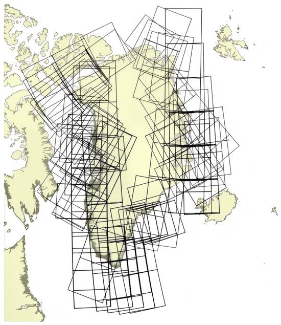
Figure 1. Spatial distribution of the scenes in the AI4Arctic/ASIP sea ice dataset.

We used only the HH and HV polarizations of SAR images for sea ice–water segmentation. We relied on the corresponding SIC charts, which are coded in SIGRID-3 (Sea Ice Geographical Reference Information and Data) format [35], to generate ground truth segmentation maps.

In a SIC chart, the polygons with a SIGRID-3 code of less than 10 (e.g., ice concentration is less than 1/10) were considered as open water, and their pixels are labeled as ‘0’, while polygons with a SIGRID-3 code between 10 and 100 are considered sea ice and their pixels are labeled as “1”.

Based on the land distance information provided in the netCDF files, all pixels located in land areas or outside the ice map boundaries are masked and excluded from model training and evaluation. Since each SAR image is large in size and cannot be directly input into the network for training, and direct downsampling would result in a significant loss of detail, we adopt a non-overlapping sliding window approach to divide the SAR images into 800 × 800 sub-regions. To improve the robustness of model training, we additionally employed standard data augmentation strategies, such as horizontal flipping, vertical flipping, and diagonal mirroring, thereby expanding the dataset to 4380 samples. These samples were then split into training, validation, and test sets following a 7:2:1 proportion. All data preprocessing procedures, including sliding window cropping and data augmentation, were implemented using Python (version 3.12.9, Python Software Foundation, Wilmington, DE, USA) and the PyTorch framework (version 2.6.0, Linux Foundation, San Francisco, CA, USA).

2.2. Proposed Method

In this section, we will provide a detailed description of the overall architecture of the proposed PFEE-UNet. We will then sequentially introduce the three core modules of the model: Cross-Polarization Channel Interaction (CPCI), Dense–Sparse Diversity Enhancement (DSDE), and Selective Edge Fusion (SEF).

Specifically, the CPCI module enhances feature separability from the data source by leveraging complementary information from different polarization channels, thereby improving the overall distinction between ice and water. The DSDE module addresses the issues of misclassification and omission caused by abrupt local texture changes by adopting parallel dense and sparse sampling strategies, with a focus on feature expression. Finally, the SEF module tackles the problem of blurred ice–water boundaries by dynamically selecting and fusing the most effective multi-scale edge features through an attention mechanism, ensuring precise control during the final stage of contour reconstruction.

2.2.1. Overall Network Architecture

To address the challenges of accurate sea ice segmentation in complex SAR scenes, we propose PFEE-UNet. As illustrated in Figure 2, the proposed architecture consists of three main components: an encoder for feature extraction, a decoder for semantic reconstruction, and an edge branch for boundary enhancement.

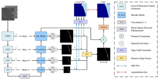
Figure 2. Overall network architecture of PFEE-UNet.

To strengthen the modeling of inter-channel semantic dependencies, a Cross-Polarization Channel Interaction module is introduced into the encoder. This module employs a grouped, staged interaction strategy: first, group-level feature enhancement is achieved through cascading convolutions, followed by inter-group cross-fusion. Finally, the interactive features are adaptively integrated to output enhanced features rich in complementary bipolar information. Furthermore, a Dense–Sparse Diversity Enhancement (DSDE) module is embedded at the bottleneck layer, where multi-scale dilated convolutions and a joint spatial-channel attention mechanism collaboratively model global context and spatial relationships, leading to further optimization of feature representation quality. The high-level features extracted by the encoder are then transmitted to the decoder via skip connections and fused with shallow-level detail features, enabling the progressive recovery of semantic information. To further improve the model’s capability in characterizing complex ice–water boundaries and contours, a multi-scale edge detection branch is introduced at the decoder stage. The output of each decoder layer $D_i$ is projected into an edge map $Ei$; then, the edge maps are input into the Selective Edge Fusion (SEF) module. The SEF module employs an adaptive attention mechanism to perform weighted fusion of multi-scale edge features. The produced edge-enhanced feature map is then concatenated with the semantic features from the final decoder output, further improving the completeness of boundary representations and sensitivity to fine-grained details. The edge map generation is supervised by an edge loss computed against the ground truth edge label, which is derived by applying morphological dilation and erosion operations to the segmentation labels.

Overall, PFEE-UNet establishes an end-to-end framework for the collaborative enhancement of polarization features and edge information. By efficiently integrating dual-polarization cues and strengthening spatial relationship modeling, the proposed network significantly improves the continuity and accuracy of sea ice boundary segmentation.

2.2.2. CPCI Module

The CPCI_Block is the core building unit of the encoder. Through a dual mechanism of grouped cascading feature enhancement and polarization cross-fusion, it not only extracts rich contextual features but also explicitly models the complementary relationship between polarizations, enhancing feature representation ability. As illustrated in Figure 3, the CPCI_Block adopts a residual structure, in which two consecutive $3\times 3$ convolutional layers enclose a dedicated Cross-Polarization Channel Interaction (CPCI) module to achieve efficient feature fusion.

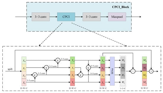
Figure 3. Architecture of the CPCI_Block module.

Existing research indicates that effective interaction between spatial and channel information is crucial for visual representation. Although current Vision Transformers enhance context modeling through spatial-channel interaction, they face two limitations in sea ice SAR image segmentation: first, they fail to fully leverage the complementary characteristics of the HH/HV dual-polarization channels, and second, the fixed-scale attention mechanism struggles to adapt to the multi-scale feature distribution of sea ice. To address these issues, and inspired by Res2Net [36] and EPSANet [37], we design the Cross-Polarization Channel Interaction (CPCI) module. This module employs a grouped cascading extraction and symmetric interaction fusion strategy: first, it uses a deep information transmission mechanism within groups to achieve feature reuse, enhancing the multi-scale representation ability within subgroups; then, it establishes symmetric inter-group feature interaction paths to explicitly mine the implicit complementary information between the HH and HV polarization channels; finally, it introduces a channel attention mechanism to dynamically recalibrate the interactive features in both spatial and channel dimensions, enabling the adaptive fusion of grouped features. This design better aligns with the polarization scattering characteristics of sea ice SAR images, significantly improving the model’s segmentation accuracy in complex scenarios by enhancing the distinction of ice–water semantic features.

For an input SAR image $X\in {\mathbb{R}}^{2\times W\times H}$, where 2 denotes the HH and HV polarization channels, and H and W represent the feature map height and width, a $3\times 3$ convolution is first applied to expand the channel dimension to C as the input to CPCI. As shown in Figure 3, $X\in {\mathbb{R}}^{C\times W\times H}$ is evenly split along the channel dimension into S sub-feature groups $\{X_1,\dots ,X_S\}$, each containing $C/S$ channels. In this work, we set $S=4$. Subsequently, each sub-feature group enters the cascading feature extraction stage. Although a uniform $3\times 3$ convolution kernel is used, we design a cross-group cascading mechanism: the output of the previous group is concatenated with the input of the next group and passed as input to the subsequent convolution layer. Compared to the original additive connection, the concatenation connection further strengthens the feature mapping capability in the spatial dimension, thereby deeply mining the implicit complementary information between the HH and HV polarization flows. This cascading design leverages feature reuse to gradually expand the effective receptive field of the network. Shallow cascading convolutions focus on preserving local edges and texture details, while with the increase in cascade depth, subsequent convolutions can capture larger structural features by utilizing accumulated contextual information. To establish deep cross-layer representation associations, we adopt a symmetric pairing logic: concatenating low-level features $Y_1$ rich in local edges and fine-grained textures with high-level features $Y_4$ that contain global contextual semantics and concatenating intermediate features $Y_2$ and $Y_3$. Each group of concatenated features undergoes deep interaction through a $5\times 5$ convolution layer. Finally, the interactive features from each group are concatenated and aggregated to build an integrated representation of multi-scale information flow, enhancing the semantic consistency and correlation between features, thus providing more discriminative feature support for subsequent sea ice target recognition.

This process can be formulated as

$$Y_1=Con{v}_{3\times 3}\left(X_1\right)$$

(1)

$$Y_i=Con{v}_{k_i\times k_i}\left(\mathrm{Cat}(X_i,Y_{i-1})\right),i=2,3,4$$

(2)

$$Y^{\prime }=\mathrm{Concat}\left(Y_4,Con{v}_{5\times 5}\left(\mathrm{Cat}(Y_4,Y_1)\right),Con{v}_{5\times 5}\left(\mathrm{Cat}(Y_3,Y_2)\right),Y_1\right)$$

(3)

Here, $Y_1$ denotes the output of the first sub-branch after the $3\times 3$ convolution. The subsequent $Y_i$ represents the output feature maps of the i-th sub-feature group, where $i=2,3,4$, corresponding to the remaining three sub-feature groups. The kernel sizes $k_i=[3,3,3]$ are assigned to $i=2,3,4$, respectively. $\mathrm{Concat}(·)$ denotes the feature concatenation operation, $Con{v}_{3\times 3}$ represents a $3\times 3$ convolution, $Con{v}_{5\times 5}$ represents a $5\times 5$ convolution, and $Y^{\prime }$ indicates the final concatenated output feature map.

Then, the channel attention mechanism (SENet) is introduced to further enhance feature discriminability. Unlike the original SENet module [38], the fully connected layers are replaced with $1\times 1$ convolutional layers, which better adapt to the structure of 2D images. Specifically, the concatenated output $Y^{\prime }$ from the sub-feature groups is globally averaged along the spatial dimensions to generate a global channel representation. This representation is then passed through two $1\times 1$ convolutional layers for dimensionality reduction and expansion in the channel dimension, combined with ReLU and Sigmoid activations, to generate the channel attention weights $W_1$, $W_5$, $W_6$, and $W_4$. Next, the generated weights are element-wise multiplied with the corresponding feature branches, resulting in recalibrated features $M_1$, $M_5$, $M_6$, and $M_4$. Through this feature recalibration operation, the model automatically enhances key features and suppresses redundant noise information. Based on this, the module further introduces learnable dynamic weight parameters, which are applied to the calibrated multi-scale features via a Softmax operation for adaptive weighting, highlighting key semantic information while effectively suppressing irrelevant background noise. Finally, the weighted fused features are added to the initial input of the CPCI module through residual connections to obtain the final output $Y_{\mathrm{out}}$. This structure not only helps preserve the original spatial details but also significantly enhances the stability of deep network training.

The process can be expressed as follows:

$$U=\mathrm{Sigmoid}\left({\mathrm{Conv}}_{1\times 1}\left(\mathrm{ReLU}\left({\mathrm{Conv}}_{1\times 1}\left(\mathrm{GAP}\left(Y^{\prime }\right)\right)\right)\right)\right)$$

(4)

$$W=\mathrm{Softmax}(\gamma \otimes U)$$

(5)

$$Y_{\mathrm{out}}=W\otimes Y^{\prime }+X$$

(6)

Here, GAP denotes the global average pooling operation, and ⊗ represents element-wise multiplication. The parameter $\gamma$ is a learnable dynamic scale weight, which is used to adaptively adjust the attention strength across different scale branches, W represents the final concatenated channel attention weights.

The combination of group-wise concatenated feature enhancement and the dynamic weighted attention mechanism not only significantly improves the model’s contextual modeling ability for complex scenes but also achieves explicit fusion of complementary HH/HV polarization channel information while maintaining computational efficiency.

The output of the CPCI module is combined with its input through a residual connection to prevent gradient vanishing. A subsequent $3\times 3$ convolution is then applied to the multi-scale, attention-enhanced features for spatial refinement while keeping the channel dimension unchanged, producing the final feature representation. After this, a $2\times 2$ max pooling operation is applied to further reduce the spatial resolution, facilitating the network’s ability to capture more abstract and high-level features while maintaining computational efficiency.

2.2.3. DSDE Module

The multi-scale features learned by the CPCI are further aggregated by the DSDE module to enhance the semantic representation of fine-grained sea ice structures. The proposed DSDE module adopts a parallel dense–sparse sampling strategy combined with joint spatial-channel attention. Compared with conventional modules, it more effectively models the spatial relationships between sea ice and seawater while enriching the diversity of local pattern representations. The architecture of the DSDE module is illustrated in Figure 4.

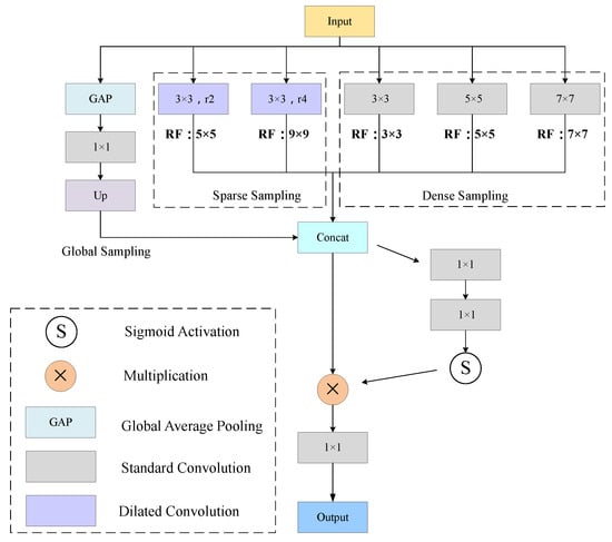
Figure 4. Architecture of the DSDE module, where the dilated convolution branches have receptive fields of 5 and 9, and the standard convolution branches have receptive fields of 3, 5, and 7.

Given an input feature map $X^{\prime }\in {\mathbb{R}}^{C\times W\times H}$, sparse sampling is realized through two dilated convolution branches. These branches employ $3\times 3$ convolution kernels with dilation rates of 2 and 4, respectively, to capture the sparse distribution characteristics of sea ice textures as well as multi-scale contextual information. Dense sampling is implemented using three convolution branches with kernel sizes of $3\times 3$, $5\times 5$, and $7\times 7$, which model local spatial correlations between sea ice and seawater and enhance the representation of complex patterns such as edges and textures.

In addition, global average pooling is applied to compress the input features to a $1\times 1$ representation, which is then broadcast to the original spatial resolution $H\times W$ to complement global dependency information.

To enable effective interaction among features from different branches, the outputs of the sparse, dense, and global sampling paths ($P_D,P_S,P_G$, respectively) are concatenated along the channel dimension, forming an aggregated feature map $F_b\in {\mathbb{R}}^{6C\times W\times H}$. This process can be expressed as follows:

$$P_D=\left[{\mathrm{Conv}}_{3\times 3}^{d=2}\left(X^{\prime }\right),{\mathrm{Conv}}_{3\times 3}^{d=4}\left(X^{\prime }\right)\right]$$

(7)

$$P_S=\left[{\mathrm{Conv}}_{3\times 3}\left(X^{\prime }\right),{\mathrm{Conv}}_{5\times 5}\left(X^{\prime }\right),{\mathrm{Conv}}_{7\times 7}\left(X^{\prime }\right)\right]$$

(8)

$$P_G=\mathrm{Up}\left({\mathrm{Conv}}_{1\times 1}\left(\mathrm{GAP}\left(X^{\prime }\right)\right)\right)$$

(9)

$$F_b=\mathrm{Concat}(P_D,P_S,P_G)$$

(10)

Here, $X^{\prime }$ denotes the input feature map. ${\mathrm{Conv}}_{k\times k}^d(·)$ represents a $k\times k$ convolution with dilation rate d, while ${\mathrm{Conv}}_{k\times k}(·)$ denotes a standard $k\times k$ convolution. $\mathrm{GAP}(·)$ indicates the operation of global average pooling. $\mathrm{Up}(·)$ denotes a spatial alignment operation used to reconcile feature map dimensions.

To further highlight key semantic information, the module incorporates a joint spatial-channel attention mechanism. Specifically, the concatenated feature $F_b$ is first passed through a $1\times 1$ convolution to reduce the channel dimension to C, followed by batch normalization and ReLU activation. It is then fed into a second $1\times 1$ convolution to expand the channels to $6C$, with a Sigmoid activation applied to generate the attention weight map A. The attention map A is multiplied element-wise with $F_b$ to adaptively enhance informative spatial-channel features while suppressing irrelevant background noise. Subsequently, the attention-enhanced features are projected to the target output channel dimension via another $1\times 1$ convolution, enabling progressive refinement of multi-scale features. The process can be expressed as follows:

$$A=\mathrm{Sigmoid}\left({\mathrm{Conv}}_{1\times 1}\left(\mathrm{ReLU}\left({\mathrm{Conv}}_{1\times 1}\left(F_b\right)\right)\right)\right)$$

(11)

$$B_{\mathrm{out}}={\mathrm{Conv}}_{1\times 1}(A\otimes F_b)$$

(12)

Here, ⊗ denotes element-wise multiplication, and $B_{\mathrm{out}}$ represents the output feature map of the DSDE module.

The combination of dense–sparse dual sampling and joint spatial-channel attention not only substantially enhances the model’s ability to capture spatial relationships in complex sea ice–water scenarios but also enables effective aggregation of multi-scale semantic information while maintaining computational efficiency. As a result, the proposed design significantly improves the representation capability for diverse fine-grained and small-scale targets.

2.2.4. SEF Module

The proposed SEF module adopts an adaptive multi-scale edge fusion strategy that integrates global feature extraction with a dynamic attention-weighting mechanism. Compared with conventional fusion approaches, SEF more effectively aggregates multi-scale edge features, enhancing the robustness and consistency of edge representations. As illustrated in Figure 5, the SEF module performs selective multi-scale edge fusion through the following steps.

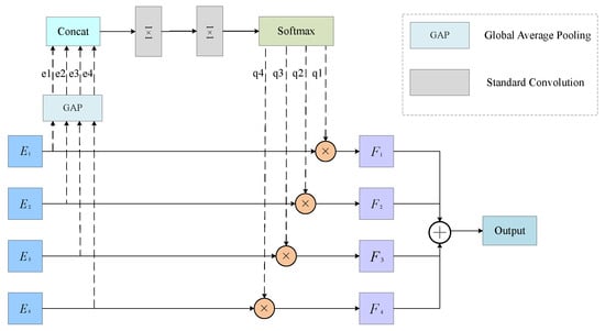
Figure 5. Architecture of the SEF module.

First, the input consists of a set of aligned edge maps from the multi-scale decoder layer, $\{E_1,E_2,E_3,E_4\}$, where each edge map is at a unified resolution $B\times 1\times H\times W$. Global average pooling is applied to each edge map to extract global features, yielding global representations with a size of $B\times 1\times 1\times 1$, which provide a scale-wise global activation summary for each edge map. Secondly, the global average responses from the four scales are concatenated along the channel dimension to form a compact multi-scale representation of size $B\times 4\times 1\times 1$. This concatenation preserves the relative activation information across scales, allowing the module to more explicitly distinguish whether a given scale provides reliable boundary cues or exhibits weaker and noisier responses. Thirdly, based on the concatenated representation, we employ a lightweight non-linear bottleneck as a learnable gating mechanism: a $1\times 1$ convolution first expands the representation to 16 channels to model cross-scale interactions in a higher-dimensional latent space; after a ReLU activation, a second $1\times 1$ convolution projects the features back to 4 channels to produce scale scores. Then, a Softmax operation is applied across the scale dimension to obtain normalized attention weights $\{q_1,q_2,q_3,q_4\}$. These weights characterize the relative importance of edge maps at different scales and are used for subsequent adaptive fusion. Finally, the SEF module performs element-wise weighted multiplication on each edge map with the attention weights and the results are accumulated to produce the fused edge map, whose size is $B\times 1\times H\times W$. The SEF module can be expressed as

$$G_i^{\prime }=GAP\left(E_i\right),i=1,2,3,4$$

(13)

$$G^{\prime }=Concat(G_1^{\prime },G_2^{\prime },G_3^{\prime },G_4^{\prime })$$

(14)

$$A^{\prime }={Conv}_{1\times 1}(\mathrm{ReLU}({\mathrm{Conv}}_{1\times 1}(G^{\prime })))$$

(15)

$$q_1,q_2,q_3,q_4=Softmax\left(A^{\prime }\right)$$

(16)

$$F_i=q_i\otimes E_i,i=1,2,3,4$$

(17)

$$F=\sum _{i=1}^4{F}_i$$

(18)

Here, $G_i^{\prime }$ denotes the global feature corresponding to the i-th edge map $E_i$. The attention weights $\{q_1,q_2,q_3,q_4\}$ are obtained by applying the Softmax function to the scale scores produced from the concatenated descriptor $G^{\prime }$, thereby adaptively quantifying the importance of each scale. The symbol ⊗ indicates element-wise multiplication, where each weight $q_i$ is broadcast across the spatial dimensions of $E_i$ to produce the weighted feature map $F_i$. Finally, the fused edge map F is obtained by accumulating these weighted feature maps across all scales.

By integrating adaptive multi-scale edge features with dynamic attention weighting, the SEF module enhances boundary representation and refinement for SAR sea ice segmentation. Moreover, the proposed gating mechanism operates on compact global descriptors and uses a lightweight weighted-fusion strategy, which efficiently exploits the complementary nature of multi-scale edge information and improves the stability and accuracy of boundary delineation.

2.2.5. Loss Function

In terms of loss design, cross-entropy (CE) loss is used as the primary segmentation loss to measure the discrepancy between the predicted results and the ground truth labels, reaching its minimum when predictions perfectly matched the ground truth. In addition, PFEE-UNet incorporates an edge enhancement mechanism. We use mean squared error (MSE) loss to constrain the accuracy of edge prediction. Specifically, the MSE loss is computed between each scale of the predicted edge map and the corresponding ground truth edge map, with equal weights. This design enhances contour awareness and boundary precision while ensuring effective optimization of the main segmentation task. The final loss function is defined as

$$\mathcal{L}={\mathcal{L}}_{\mathrm{Seg}}+\lambda {\mathcal{L}}_{\mathrm{Edge}}.$$

(19)

$${\mathcal{L}}_{\mathrm{Seg}}=\mathrm{CE}(\widehat{Y},Y)$$

(20)

$${\mathcal{L}}_{\mathrm{Edge}}=\sum _{i=1}^4{\parallel E_i,Y_{edg}\parallel }_2$$

(21)

where $\lambda =0.1$ is the combination weight, determined experimentally; $\widehat{Y}$ and Y represent the predicted segmentation result and the ground truth label, respectively; $Y_{edg}$ represents the ground truth edge map.

3. Experiment and Results

3.1. Evaluation Metrics

To evaluate the performance of the proposed model, we employ several quantitative metrics, including overall accuracy (OA), Mean Intersection over Union (mIoU), precision, recall, and F1 score (F1), to enable a comprehensive comparison with existing state-of-the-art methods. These metrics are computed based on the basic parameters of cumulative confusion matrix:

• TP: True Positive—the number of correctly classified ice pixels as ice.
• TN: True Negative—the number of correctly classified water pixels as water.
• FP: False Positive—the number of water pixels misclassified as ice.
• FN: False Negative—the number of ice pixels misclassified as water.

Based on these parameters, the evaluation metrics are defined as follows:

OA measures the proportion of correctly classified pixels (both ice and water) out of all the pixels in the image.

$$\mathrm{OA}={\displaystyle \frac{TP+TN}{TP+TN+FP+FN}}$$

(22)

mIoU computes the average ratio of intersection to union between the predicted and true segmentation masks for ice and water.

$$\mathrm{mIoU}={\displaystyle \frac{1}{2}}\left({\displaystyle \frac{TP}{TP+FP+FN}}+{\displaystyle \frac{TN}{TN+FP+FN}}\right)$$

(23)

Precision measures the proportion of correctly predicted ice pixels out of all pixels predicted as ice.

$$\mathrm{precision}={\displaystyle \frac{TP}{TP+FP}}$$

(24)

Recall measures the proportion of correctly predicted ice pixels out of all actual ice pixels.

$$\mathrm{recall}={\displaystyle \frac{TP}{TP+FN}}$$

(25)

F1 score is the harmonic mean of precision and recall, providing a balance between them.

$$\mathrm{F}1=2\times {\displaystyle \frac{\mathrm{precision}\times \mathrm{recall}}{\mathrm{precision}+\mathrm{recall}}}$$

(26)

3.2. Experimental Settings

All models were trained and validated using the PyTorch framework (version 2.6.0) with CUDA 11.8, on an NVIDIA GeForce RTX 4090 GPU with 24 GB of VRAM. Batch size was set to 4. The AdamW optimizer was employed with a weight decay of $1\times {10}^{-4}$. The learning rate was dynamically adjusted using a cosine annealing schedule, with an initial learning rate of $5\times {10}^{-5}$ and a minimum learning rate decayed to approximately $1\times {10}^{-6}$. To prevent overfitting and improve training efficiency, an early stopping strategy was applied, with a maximum of 100 training epochs and a patience of 10; training was terminated when the validation mIoU showed no improvement for 10 consecutive epochs.

3.3. Quantitative Results

To demonstrate the superiority of PFEE-UNet, we compared it with several state-of-the-art semantic segmentation methods on the AI4Arctic dataset. The results are presented in Table 1. The comparison methods includes classic CNN-based frameworks such as U-Net, DeepLabV3+, and HRNet, as well as Transformer-based variants like SwinUNet and SegFormer. In addition, hybrid CNN–Transformer architectures, including CMTFNet [39] and SRCBTFusion-Net [40], were also included to comprehensively evaluate the competitiveness of PFEE-UNet.

Table 1. Comparative experimental results of different segmentation models. All scores are expressed as percentages (%), and the evaluation metric for all categories is mIoU.

Models	Sea Ice	Water	mIoU	Mean F1	OA
CMLFormer [41]	80.71	83.54	82.12	88.76	92.90
CMTFNET [39]	80.61	82.92	81.76	88.59	92.80
DeepLabv3+ [42]	81.22	83.57	82.40	88.97	93.07
HRNet [26]	81.19	83.64	82.52	89.11	93.14
MsanlfNet [43]	81.08	82.78	81.93	88.76	92.80
SwinUnet [28]	79.95	82.84	81.40	88.30	92.67
SegFormer [27]	81.03	83.04	82.04	88.75	92.85
TransUNet [44]	73.82	76.02	74.92	81.55	92.10
UNet [45]	79.22	81.39	80.31	87.64	91.79
SRCBTFusion-Net [40]	80.39	82.86	81.62	88.39	92.65
MMSeaIceUNet [46]	77.03	80.53	78.78	86.66	91.03
PFEE-UNet (Ours)	83.61	85.36	84.48	90.55	94.02

Note: The best values in the columns are shown in bold.

As shown in Table 1, the proposed PFEE-UNet achieves the best performance in the sea ice and water segmentation task, with an mIoU of $84.48\%$, mean F1 of $90.55\%$, and OA of $94.02\%$. Compared to the second-best method, PFEE-UNet improves mIoU by $1.96\%$, mean F1 by $1.44\%$, and OA by $0.88\%$. These results clearly demonstrate the strong capability of our model in preserving sea ice contours and effectively distinguishing pixel-level differences between sea ice and open water in SAR imagery.

3.4. Visual Comparison

Although numerical metrics provide a summary of model accuracy, visual analysis offers a more intuitive means of evaluating model performance. In this study, we selected several representative test images from diverse spatio-temporal contexts to demonstrate the effectiveness of different models. Figure 6 presents the segmentation results for a sample acquired from the Southern Greenland region (Cape Farewell) on 4 April 2019. This scene represents a typical marginal ice zone (MIZ) with highly fragmented ice and narrow leads, providing a rigorous benchmark for evaluating fine structural preservation.

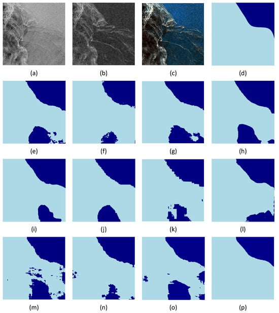
Figure 6. Visualization of different methods on the AI4Arctic dataset, sample acquired on 4 April 2019 from the Southern Greenland region (Cape Farewell). (a) Original SAR image (HH), (b) original SAR image (HV), (c) SAR pseudo-color image (R channel: HH, G channel: HV, B channel: average of HH and HV). (d) Ground truth segmentation map (dark blue for open water, light blue for sea ice), (e) CMLFormer, (f) CMTFNet, (g) DeepLabv3+, (h) HRNet, (i) MsanlfNet, (j) SwinUNet, (k) SegFormer, (l) TransUNet, (m) UNet, (n) SRCBTFusion, (o) MMSeaIceUNet, and (p) PFEE-UNet (Ours).

Based on the visual results in Figure 6, the proposed PFEE-UNet demonstrates clear advantages in sea ice segmentation on SAR images (both HH and HV polarizations). Compared to other methods such as CMLFormer, CMTFNet, and DeepLabv3+, PFEE-UNet can more accurately distinguish sea ice from open water in complex speckle backgrounds, effectively reducing the misclassification of water as ice. Notably, in areas with broken ice and narrow ice leads at the bottom of the images, other methods often misclassify sea ice as water or fail to detect it under high-noise, low-contrast conditions, resulting in obvious gaps and structural loss in the predicted masks. In contrast, PFEE-UNet is able to reconstruct the ice distribution in these regions more completely, producing predictions that closely match the ground truth in terms of boundary continuity and shape preservation. This significantly reduces both misclassification and omission, highlighting the model’s superiority in edge retention and overall ice–water segmentation accuracy.

Figure 7 shows another set of results from the SAR image at the South West Greenland region (30 March 2019), characterized by blurred boundaries and similar backscatter intensities between ice and water. This region poses a high demand on the model’s edge detection capability. It can be observed that SegFormer (Figure 7k) exhibits noticeable misclassification, with incomplete ice contours. DeepLabV3+ (Figure 7g) and HRNet (Figure 7h) show some improvement but still struggle with ice–water confusion along complex edges. Other methods, such as CMLFormer and CMTFNet, continue to misidentify local sea ice as water in low-contrast areas. In contrast, the proposed PFEE-UNet (Figure 7p) achieves better segmentation consistency and robustness, highlighting its superiority in handling low-density transition regions and maintaining edge integrity.

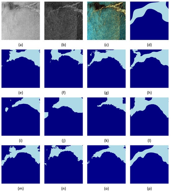
Figure 7. Visualization results of different methods on the AI4Arctic dataset, sample acquired on 30 March 2019 from the South West Greenland region. (a) Original SAR image (HH). (b) Original SAR image (HV). (c) SAR pseudo-color image (R channel: HH, G channel: HV, B channel: average of HH and HV). (d) Ground truth segmentation map (dark blue for open water, light blue for sea ice), (e) CMLFormer, (f) CMTFNet, (g) DeepLabv3+, (h) HRNet, (i) MsanlfNet, (j) SwinUNet, (k) SegFormer, (l) TransUNet, (m) UNet, (n) SRCBTFusion, (o) MMSeaIceUNet, and (p) PFEE-UNet (Ours).

Its predictions closely match the ground truth (Figure 7d), with clearer and more complete ice–water boundaries, effectively reducing misclassification and edge blurring. These results highlight the superior performance of PFEE-UNet in high-resolution sea ice segmentation tasks.

3.5. Ablation Study

To thoroughly investigate the contributions of each component in PFEE-UNet, we adopted the standard U-Net as the baseline model and incrementally incorporated the Cross-Polarization Channel Interaction (CPCI) module, the Dense–Sparse Spatial Feature Enhancement (DSDE) module, the Edge Enhancement (EE) component, and the Selective Edge Fusion (SEF) module into the base architecture. Ablation experiments were then conducted to systematically evaluate the effectiveness of each module. Specifically, to assess the impact of the SEF module, in the ablation study, edge fusion in the EE component without SEF was implemented using simple feature concatenation (Concat) as a comparison.

The ablation results are summarized in Table 2. Figure 8 provides the corresponding visual comparisons based on a representative winter ice sample (South West Greenland, 1 March 2019). Additionally, Grad-CAM visualizations were used to generate heatmaps for the CPCI, DSDE modules, and encoder features in Figure 9. This figure evaluates feature enhancement across two distinct scenarios—a stable ice cover (Central West Greenland, 2 December 2018) and a fragmented marginal ice zone (Cape Farewell, 4 April 2019)—to demonstrate the model’s adaptability.

Table 2. Ablation study results of PFEE-UNet components.

Models	Baseline	+CPCI	+DSDE	+EE (cat)	+SEF	mIoU (%)	OA (%)	F1 (%)
A	√	×	×	×	×	79.13	90.88	86.51
B	√	√	×	×	×	82.97	93.30	89.54
C	√	√	√	×	×	83.37	93.53	89.62
D	√	√	√	√	×	83.85	93.87	89.87
E	√	√	√	×	√	84.48	94.02	90.55

Note: The best values in each column are shown in bold.

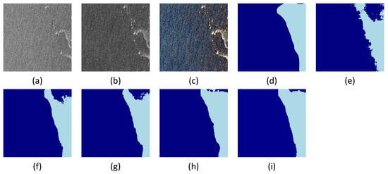
Figure 8. Visualization of the ablation study on the AI4Arctic dataset; sample acquired on 1 March 2019 from the South West Greenland region. (a) Original SAR image (HH). (b) Original SAR image (HV). (c) SAR pseudo-color image. (d) Ground truth semantic segmentation map. (e) Model A in Table 2, (f) Model B, (g) Model C, (h) Model D, and (i) Model E.

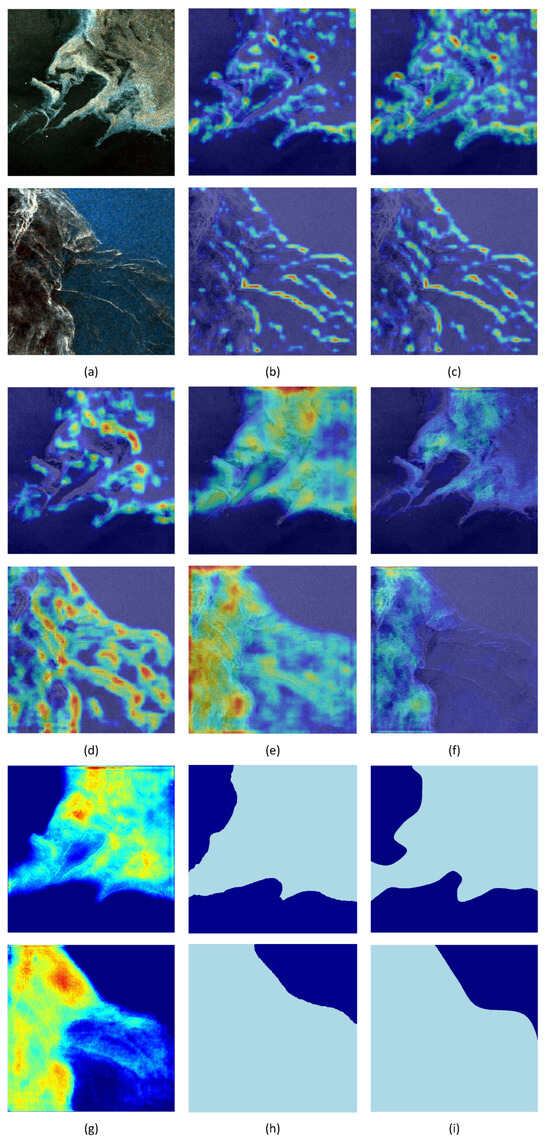
Figure 9. Visualization analysis of feature maps. (a) SAR pseudo-color images, where the first row shows a sample from the Central West Greenland region (2 December 2018) and the second row shows a sample from the Southern Greenland region (Cape Farewell, 4 April 2019). (b) Before incorporating CPCI features. (c) After incorporating CPCI features. (d) Before incorporating DSDE. (e) After incorporating DSDE. (f) Before incorporating Edge Enhancement module. (g) After incorporating Edge Enhancement module. (h) Segmentation result. (i) Ground truth semantic segmentation map.

First, incorporating the CPCI module significantly improved all evaluation metrics: mIoU increased from 79.13% to 82.97%, mean F1 rose from 86.51% to 89.54%, and OA increased from 90.88% to 93.30%. This indicates that CPCI, through its group-wise concatenation and interaction strategy, deeply mines and integrates the complementary features from the dual-polarization input. By leveraging the deep information transfer mechanism brought by inter-group concatenation and the feature interaction strategy, the module effectively enhances the model’s ability to distinguish between sea ice and open water. To further validate this conclusion, we visualized the results of the CPCI module, as shown in Figure 8f. Thanks to CPCI’s hierarchical feature perception and cross-group interaction fusion mechanism, the network’s ability to suppress complex SAR image backgrounds is significantly improved, particularly excelling in handling blurred ice–water boundaries.

Furthermore, the incorporation of the DSDE module further improved all evaluation metrics, with the mIoU increasing from 82.97 to 83.37. As shown in Figure 8g, the DSDE module optimized the segmentation results, enhancing the model’s ability to capture local texture details. This effectively alleviated the misclassification and omission issues caused by abrupt changes in local textures, thanks to its joint optimization of multi-scale dilated convolutions and spatial relationship branches.

Subsequently, the Edge Enhancement (EE) module optimizes the boundary fidelity of segmentation by strengthening the feature representation of sea ice edges. Its core principle lies in applying adaptive feature enhancement to specifically address the complex noise at ice–water interfaces in SAR images, thereby improving edge continuity and clarity. Figure 8h illustrates its effect, showing that incorporating this module significantly refines the segmentation, producing smoother and more accurate boundaries between sea ice and open water.

Furthermore, the SEF module employs a Selective Edge Fusion strategy, effectively leveraging multi-scale edge features to enhance the model’s boundary recognition capability. This approach mitigates common issues in sea ice segmentation, such as blurred or discontinuous edges, resulting in final segmentation outputs with significantly improved boundary clarity and contour integrity (see Figure 8i), thereby validating the effectiveness of the SEF module.

Finally, Grad-CAM visualization is used to systematically validate the synergistic effects of the overall PFEE-UNet and its key modules from an interpretability perspective. For all visualization experiments in this section, we calculate the gradient contributions of feature maps to the target class prediction scores to highlight the regions that most strongly influence the model’s decisions. The resulting heatmaps are overlaid on the original remote sensing images to intuitively display the spatial distribution of model attention.

(a) CPCI ablation visualization: To explore the role of the CPCI module in feature extraction, we compared the visualizations of feature maps with and without CPCI. The visualization focused on the last CPCI_Block module in the encoder, located in the deeper network layers with strong semantic aggregation and high-level feature representation, reflecting global attention distribution and response intensity. As shown in Figure 9b, without CPCI, attention is dispersed and response strength is reduced, weakening the model’s focus on the main sea ice structures, with some edge regions showing activation loss. After introducing CPCI (Figure 9c), high-response areas expand significantly, with attention concentrated on the main sea ice body and continuous edge regions. This demonstrates that CPCI plays a crucial role in cross-polarization channel feature interaction, enhancing the model’s response to semantically significant regions and improving feature discriminability and stability.

(b) DSDE ablation visualization: As shown in Figure 9d, without the DSDE module, the model’s high-response regions are limited to the edges of sea ice and cracks, focusing on local textures and neglecting the overall shape and spatial distribution. This leads to fragmented feature representation and hinders stable global semantic perception. After the introduction of the DSDE module, the decision heatmap of the full model (Figure 9e) reveals a significant expansion of the response range at the bottleneck layer. Since the bottleneck layer is located at the deepest part of the encoder and contains the highest-dimensional abstract semantic information, the high spatial consistency between the heatmap and the final semantic segmentation mask is crucial.

Experimental observations show that high-attention areas precisely cover the sea ice body, while seawater regions exhibit very low activation, and background noise is effectively suppressed. This “deep feature-output mask” synchronization indicates that the model’s decision-making process is based on a deep semantic understanding of the overall sea ice morphology, rather than relying on shallow, low-level textures or noise. Driven by this, the model shows significant advantages in spatial continuity and boundary integrity, validating the DSDE module’s key role in enhancing small-scale structure recognition and modeling complex ice–water relationships, ultimately improving feature extraction effectiveness and segmentation result reliability.

(c) Edge Enhancement Module Ablation Visualization: To better understand the role of the edge enhancement module in the feature extraction stage, we compared the heatmaps with and without the module. As shown in Figure 9f, without the edge enhancement module, the heatmap clearly displays dispersed attention areas with lower response strength, which leads to insufficient focus on the sea ice body structure. Additionally, some sea ice edges lack activation, resulting in incomplete boundary information. After introducing the edge enhancement module, as shown in Figure 9g, the high-response areas at the same layer significantly expand, with attention focused on the sea ice body and its continuous edge regions. The boundary activation becomes clearer and more continuous. This indicates that the edge enhancement module plays a crucial role in guiding the fusion of edge information, contributing significantly to the cross-scale integration of edge information within the model. As a result, it enhances the model’s ability to respond to semantically significant areas and boundary information. In this way, the edge enhancement module greatly improves the discriminative power and stability of feature representation, ultimately improving segmentation performance.

3.6. Loss Function Weight Experiment

To evaluate the impact of edge loss weight $\lambda$ on model performance, we conducted experiments with different weight settings, ranging from 0.05 to 0.5. In all experiments, the main segmentation loss was fixed as cross-entropy loss (CE), while the weight of the edge loss was gradually adjusted. The experimental results showed that when the edge loss weight was set to 0.1, the model achieved the best balance between segmentation accuracy (OA) and boundary precision (mIoU).

As shown in Table 3, setting the edge loss weight to 0.1 resulted in the highest performance, with sea ice and water segmentation performances of 83.61% and 85.36%, respectively. The model also achieved an mIoU of 84.48% and a mean F1 score of 90.55%. Based on these results, we selected 0.1 as the optimal edge loss weight for better overall segmentation accuracy and boundary precision.

Table 3. Comparative experimental results of different edge loss weights. All scores are expressed as percentages (%).

Weight ($\mathit{\lambda }$)	Sea ice	Water	mIoU	Mean F1
0.05	82.80	84.93	83.87	90.10
0.1	83.61	85.36	84.48	90.55
0.2	82.96	84.69	83.82	90.05
0.5	80.60	83.85	82.23	88.88

Note: The best values in the columns are shown in bold.

3.7. Complexity Analysis

To comprehensively evaluate the efficiency and performance of different networks, we conducted comparative experiments on the AI4Arctic dataset under identical operating conditions. All models were trained and tested with input images of size $224\times 224$, a batch size of 1, and two input channels. The experiments were carried out on a PyTorch (version 2.6.0) platform with an NVIDIA GeForce RTX 4090 D (24 GB VRAM) under CUDA 11.8. To ensure fairness and stability, all tests involved GPU memory clearing and multiple repeated measurements. The results are summarized in Table 4.

Table 4. Comparison of model complexity and segmentation performance across different networks.All scores are expressed as percentages (%).

Models	Params (M)	FLOPs (G)	mIoU	Mean F1
CMLFormer [41]	12.53	3.78	82.12	88.76
CMTFNET [39]	30.07	6.84	81.76	88.59
DeepLabv3+ [42]	39.75	33.10	82.40	88.97
HRNet [26]	65.85	17.92	82.52	89.11
MsanlfNet [43]	34.95	5.26	81.93	88.76
SwinUnet [28]	27.16	12.04	81.40	88.30
SegFormer [27]	43.29	13.75	82.04	88.75
TransUNet [44]	105.32	37.13	74.92	81.55
UNet [45]	31.04	36.90	80.31	87.64
SRCBTFusion-Net [40]	103.67	17.46	81.62	88.39
MMSeaIceUNet [46]	0.49	1.93	78.78	86.66
PFEE-UNet (Ours)	42.68	19.98	84.48	90.55

Note: The best values in the columns are shown in bold.

PFEE-UNet is an improvement on the UNet network architecture. Compared to the baseline model UNet, although the number of parameters has increased to some extent (11.64 M), the computational complexity has decreased by approximately 46%, and the segmentation performance has improved significantly (mIoU increased by 4.17%). The models with the closest segmentation performance to PFEE-UNet are HRNet and DeepLabv3+. They are respectively higher than our model in terms of the number of parameters and computational complexity. MMSeaIceUNet has the smallest number of parameters and computational complexity, which benefits from its streamlined network structure, but the gap in segmentation results is relatively large. Overall, the proposed model achieves notable performance gains at a reasonable computational cost, particularly excelling in terms of mIoU. In the future, we will improve its computational efficiency through model lightweighting.

4. Discussion

4.1. Real-World SAR Scenario Application

A high-quality automatic sea ice segmentation model not only provides near-real-time capabilities for sea ice charting but also significantly reduces the influence of human decision biases. To comprehensively evaluate the model’s generalization performance and operational robustness in real-world scenarios, it is essential to conduct tests on actual SAR imagery.

To validate the practicality of the proposed PFEE-UNet in large-scale real-world SAR images, the trained model was directly applied to segment ice–water regions in complete SAR scenes, achieving end-to-end ice–water segmentation. The specific workflow consists of three steps:

• First, the full SAR image is read, and mean–standard deviation normalization is applied to the polarization channels based on the training set statistics to mitigate distribution shifts caused by varying imaging conditions. The image is then cropped into fixed $800\times 800$ patches with a 50% overlap to enhance prediction stability along patch edges.
• Each cropped patch is fed sequentially into PFEE-UNet for inference. For overlapping regions, probability maps are aggregated with weighted accumulation and normalized to obtain consistent global predictions.
• The probability maps are then mapped back according to patch positions to reconstruct the complete scene. Gaussian smoothing and morphological opening–closing operations are applied to further enhance the continuity and clarity of ice–water boundaries.

For qualitative analysis, a full dual-polarization SAR scene acquired on 6 November 2025, over the northeastern region of Greenland—outside the training and validation sets—was selected. Figure 10a shows an overview map of Greenland and surrounding areas, with the red rotated rectangle indicating the coverage of this scene.

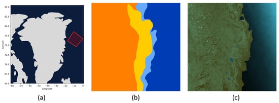
Figure 10. Application of PFEE-UNet for ice–water segmentation on SAR images. (a) SAR image near the northeastern coast of Greenland on 6 November 2025. (b) DMI sea ice analysis chart, where dark blue represents open water (ice concentration < 1/10), light blue represents 1–3/10 ice concentration, green represents 4–6/10 ice concentration, yellow represents 7–8/10 ice concentration, and orange represents 9–10/10 ice concentration. (c) Predicted segmentation results overlaid on the SAR image, with brownish-yellow on the left representing sea ice and bluish-green on the right representing open water.

As a reference, Figure 10b presents the sea ice analysis chart released by the Danish Meteorological Institute (DMI), which follows the WMO-standard ice concentration classification system. Although ice charts are subjective products derived from multi-source data and vary across operational agencies, they represent the best available standard in operational sea ice monitoring. We use this chart as a standardized operational reference to provide a qualitative benchmark for evaluating the model’s segmentation performance in large-scale, unseen scenarios. Figure 10c shows the PFEE-UNet segmentation results on the original SAR image, demonstrating that the model can stably capture large-scale boundaries between sea ice and open water. The overall segmentation contours closely align with the ice edge positions defined in the reference chart, indicating that the model maintains strong generalization capability in unseen scenarios.

The results indicate that PFEE-UNet maintains stable segmentation performance in entirely unseen scenarios, demonstrating its generalization ability and engineering value for practical applications. To quantify the model’s performance in real SAR scenes, this study performed pixel-wise evaluation of the segmentation results from PFEE-UNet using the DMI reference ice map and computed metrics such as sea ice IoU, seawater IoU, and mIoU. Overall, PFEE-UNet achieved excellent results in terms of sea ice IoU, seawater IoU, and mIoU, with values of 98.27%, 96.65%, and 97.46%, respectively, while the overall accuracy reached 98.85%. Nevertheless, since this evaluation relies on binarized operational sea ice products as reference labels, it is also necessary to discuss the inherent uncertainties associated with the ground truth used in both training and real-scene assessment.

4.2. Ground Truth Discussion

It is important to note that the use of binarized sea ice concentration (SIC) products as ground truth for model training introduces certain uncertainties. First, the threshold used to binarize SIC (set at 10% in this study) could significantly impact the delineation of the ice–water boundary. Nevertheless, this threshold is widely adopted in both operational sea ice mapping and academic research. The World Meteorological Organization’s Sea Ice Terminology (WMO No. 259) defines ice-free areas as having a concentration of less than 10%. Furthermore, Haarpaintner and Spreen [47] showed that satellite data can detect sea ice concentrations as low as 10%.

Another source of uncertainty arises from mixed pixels, particularly in the marginal ice zone, where a single pixel may simultaneously contain both ice and water. During binarization, such pixels are inevitably assigned to only one category, which introduces noise into the ground truth. However, we emphasize that the SIC used in this study originates from the manually interpreted operational ice charts produced by the Danish Meteorological Institute (DMI), rather than from an automatically retrieved SIC product. These charts represent a widely accepted operational reference for navigation and climate research. Although they are not exhaustive physical representations, they serve as a standardized benchmark in the field and provide a reliable and practical basis for training segmentation models intended to automate the ice charting process.

In addition, SIC products themselves contain inherent inversion errors, which are further propagated into the binarized labels. Despite these challenges, we consider the resulting ground truth suitable for model training for two main reasons. First, the primary objective of this study is to develop a model that learns from operational sea ice mapping practices, which inherently rely on the 10% threshold and expert interpretation. Second, the noise introduced by thresholding and mixed pixels is alleviated by the large and diverse training dataset, which consists of 461 Sentinel-1 scenes spanning wide spatial and temporal variations. Such diversity enables the model to learn robust and transferable features even under imperfect supervision.

Despite these limitations, the experimental results show that the model maintains high consistency with manually interpreted references on both the test set and unseen real SAR scenes. This indicates that the model is able to learn meaningful feature representations and accurately delineate ice–water boundaries, even when trained with imperfect or noisy labels. These findings further demonstrate the robustness of the proposed method and support its potential for practical applications.

5. Conclusions

In this study, we propose a novel edge-enhanced sea ice segmentation network, termed PFEE-UNet, specifically designed for precise sea ice delineation in high-resolution SAR images. The proposed network introduces a Cross-Polarization Channel Interaction (CPCI) module to improve the encoder’s feature representation capability. By employing inter-group cascade extraction and cross-group interactive fusion, the CPCI module explicitly explores the complementarity between HH and HV channels; while HH polarization is highly sensitive to surface roughness, HV responds effectively to volume scattering from deformed ice. This mechanism allows the network to maximize mutual information between channels, thereby significantly enhancing the distinction between sea ice and open water. Meanwhile, the Dense–Sparse Diversity Enhancement (DSDE) module leverages multi-scale dilated convolution branches and spatial relationship modeling to strengthen spatial dependency and local pattern diversity. From an information-processing perspective, this compensates for the textural heterogeneity of sea ice across different scales. Additionally, the Selective Edge Fusion (SEF) module integrates multi-scale edge information, significantly improving boundary continuity and structural integrity in the segmentation results.

Extensive experiments conducted on the AI4Arctic/ASIP sea ice dataset demonstrate that PFEE-UNet consistently outperforms existing mainstream methods. Despite these strengths, the method operates under the fundamental assumption that dual-polarization inputs are geometrically co-registered and lacks extreme meteorological interference, such as heavy rain, which can alter surface backscatter. Future work will focus on further optimizing the lightweight design of the network and improving its generalization capability, while addressing the challenges posed by complex boundary conditions. These efforts are expected to better support polar navigation safety and marine environmental monitoring. In addition, future research will extend the current framework to multi-class sea ice classification tasks and explore this direction in a more comprehensive manner.

References

- Andersson, T.R.; Hosking, J.S.; Pérez-Ortiz, M.; Paige, B.; Elliott, A.; Russell, C.; Law, S.; Jones, D.C.; Wilkinson, J.; Phillips, T.; et al. Seasonal Arctic sea ice forecasting with probabilistic deep learning. Nat. Commun. 2021, 12, 5124. [Google Scholar] [CrossRef]
- Alkaee Taleghan, S.; Barrett, A.P.; Meier, W.N.; Banaei-Kashani, F. IceBench: A Benchmark for Deep-Learning-Based Sea-Ice Type Classification. Remote Sens. 2025, 17, 1646. [Google Scholar] [CrossRef]
- Zhou, L.; Zheng, S.; Ding, S.; Xie, C.; Liu, R. Influence of propeller on brash ice loads and pressure fluctuation for a reversing polar ship. Ocean Eng. 2023, 280, 114624. [Google Scholar] [CrossRef]
- Song, W.; Li, H.; He, Q.; Gao, G.; Liotta, A. E-mpspnet: Ice–water sar scene segmentation based on multi-scale semantic features and edge supervision. Remote Sens. 2022, 14, 5753. [Google Scholar] [CrossRef]
- Malmgren-Hansen, D.; Pedersen, L.T.; Nielsen, A.A.; Kreiner, M.B.; Saldo, R.; Skriver, H.; Lavelle, J.; Buus-Hinkler, J.; Krane, K.H. A convolutional neural network architecture for Sentinel-1 and AMSR2 data fusion. IEEE Trans. Geosci. Remote Sens. 2020, 59, 1890–1902. [Google Scholar] [CrossRef]
- Ren, Y.; Li, X.; Yang, X.; Xu, H. Development of a dual-attention U-Net model for sea ice and open water classification on SAR images. IEEE Geosci. Remote Sens. Lett. 2021, 19, 4014005. [Google Scholar] [CrossRef]
- Holmes, Q.A.; Nuesch, D.R.; Shuchman, R.A. Textural analysis and real-time classification of sea-ice types using digital SAR data. IEEE Trans. Geosci. Remote Sens. 2007, 45, 113–120. [Google Scholar] [CrossRef]
- Wang, Q.; Lohse, J.P.; Doulgeris, A.P.; Eltoft, T. Data augmentation for SAR sea ice and water classification based on per-class backscatter variation with incidence angle. IEEE Trans. Geosci. Remote Sens. 2023, 61, 1–15. [Google Scholar] [CrossRef]
- Al-Bayati, M.; El-Zaart, A. Automatic thresholding techniques for SAR images. In Proceedings of the International Conference of Soft Computing, Dubai, United Arab Emirates, 2–3 December 2013; pp. 2–3. [Google Scholar]
- Guo, W.; Itkin, P.; Lohse, J.; Johansson, M.; Doulgeris, A.P. Cross-platform classification of level and deformed sea ice considering per-class incident angle dependency of backscatter intensity. Cryosphere 2022, 16, 237–257. [Google Scholar] [CrossRef]
- Cristea, A.; Van Houtte, J.; Doulgeris, A.P. Integrating incidence angle dependencies into the clustering-based segmentation of SAR images. IEEE J. Sel. Top. Appl. Earth Obs. Remote Sens. 2020, 13, 2925–2939. [Google Scholar] [CrossRef]
- Moen, M.A.N.; Doulgeris, A.P.; Anfinsen, S.N.; Renner, A.H.H.; Hughes, N.; Gerland, S.; Eltoft, T. Comparison of feature based segmentation of full polarimetric SAR satellite sea ice images with manually drawn ice charts. Cryosphere 2013, 7, 1693–1705. [Google Scholar] [CrossRef]
- Yu, Z.; Wang, T.; Zhang, X.; Zhang, J.; Ren, P. Locality preserving fusion of multi-source images for sea-ice classification. Acta Oceanol. Sin. 2019, 38, 129–136. [Google Scholar] [CrossRef]
- Leigh, S.; Wang, Z.; Clausi, D.A. Automated ice–water classification using dual polarization SAR satellite imagery. IEEE Trans. Geosci. Remote Sens. 2013, 52, 5529–5539. [Google Scholar] [CrossRef]
- Park, J.W.; Korosov, A.A.; Babiker, M.; Won, J.S.; Hansen, M.W.; Kim, H.C. Classification of sea ice types in Sentinel-1 SAR images. Cryosphere 2019, 13, 3201–3223. [Google Scholar]
- Zhang, Y.; Zhu, T.; Spreen, G.; Melsheimer, C.; Huntemann, M.; Hughes, N.; Zhang, S.; Li, F. Sea ice and water classification on dual-polarized Sentinel-1 imagery during melting season. Cryosphere 2021, 15, 4909–4934. [Google Scholar]
- Rogers, M.S.J.; Fox, M.; Fleming, A.; van Zeeland, L.; Wilkinson, J.; Hosking, J.S. Sea ice detection using concurrent multispectral and synthetic aperture radar imagery. Remote Sens. Environ. 2024, 305, 114073. [Google Scholar] [CrossRef]
- Niu, L.; Tang, X.; Yang, S.; Zhang, Y.; Zheng, L.; Wang, L. Detection of Antarctic surface meltwater using Sentinel-2 remote sensing images via U-net with attention blocks: A case study over the Amery Ice Shelf. IEEE Trans. Geosci. Remote Sens. 2023, 61, 4204613. [Google Scholar] [CrossRef]
- Chen, X.; Patel, M.; Xu, L.; Chen, Y.; Scott, K.A.; Clausi, D.A. A Weakly Supervised Learning Approach for Sea Ice Stage of Development Classification From AI4Arctic Sea Ice Challenge Dataset. IEEE Trans. Geosci. Remote Sens. 2025, 63, 4202915. [Google Scholar] [CrossRef]
- Zhang, Z.; Deng, G.; Luo, C.; Li, X.; Ye, Y.; Xian, D. A multiscale dual attention network for the automatic classification of polar sea ice and open water based on Sentinel-1 SAR images. IEEE J. Sel. Top. Appl. Earth Obs. Remote Sens. 2024, 17, 5500–5516. [Google Scholar] [CrossRef]
- Zhang, C.; Chen, X.; Ji, S. Semantic image segmentation for sea ice parameters recognition using deep convolutional neural networks. Int. J. Appl. Earth Obs. Geoinf. 2022, 112, 102885. [Google Scholar] [CrossRef]
- Sun, S.; Wang, Z.; Tian, K. Fine extraction of Arctic sea ice based on CA-DeepLabV3+ model. In Proceedings of the Second International Conference on Geographic Information and Remote Sensing Technology, Nanjing, China, 22–24 September 2023; SPIE: Bellingham, WA, USA, 2023; Volume 12797, pp. 435–440. [Google Scholar]
- Song, W.; Zhu, M.; Ge, M.; Liu, B. A Shape-Aware Network for Arctic Lead Detection from Sentinel-1 SAR Images. J. Mar. Sci. Eng. 2024, 12, 856. [Google Scholar] [CrossRef]
- Ma, T.; Chen, X.; Xu, L.; Ma, P.; Yu, P. MFGC-Net: Bridging and fusing multiscale features and global contexts for multi-task sea ice fine segmentation. IEEE J. Sel. Top. Appl. Earth Obs. Remote Sens. 2025, 18, 14015–14035. [Google Scholar] [CrossRef]
- Hu, W.; Wang, X.; Zhan, F.; Cao, L.; Liu, Y.; Yang, W.; Ji, M.; Meng, L.; Guo, P.; Yang, Z.; et al. OPT-SAR-MS2Net: A multi-source multi-scale siamese network for land object classification using remote sensing images. Remote Sens. 2024, 16, 1850. [Google Scholar] [CrossRef]
- Wang, J.; Sun, K.; Cheng, T.; Jiang, B.; Deng, C.; Zhao, Y.; Liu, D.; Mu, Y.; Tan, M.; Wang, X.; et al. Deep high-resolution representation learning for visual recognition. IEEE Trans. Pattern Anal. Mach. Intell. 2020, 43, 3349–3364. [Google Scholar] [CrossRef] [PubMed]
- Xie, E.; Wang, W.; Yu, Z.; Anandkumar, A.; Alvarez, J.M.; Luo, P. SegFormer: Simple and efficient design for semantic segmentation with transformers. Adv. Neural Inf. Process. Syst. 2021, 34, 12077–12090. [Google Scholar]
- Cao, H.; Wang, Y.; Chen, J.; Jiang, D.; Zhang, X.; Tian, Q.; Wang, M. Swin-unet: Unet-like pure transformer for medical image segmentation. In Proceedings of the European Conference on Computer Vision, Tel Aviv, Israel, 23–27 October 2022; Springer: Cham, Switzerland, 2022; pp. 205–218. [Google Scholar]
- Zhang, J.; Zhang, W.; Zhou, X.; Chu, Q.; Yin, X.; Li, G.; Dai, X.; Hu, S.; Jin, F. CNN and transformer fusion network for sea ice classification using Gaofen-3 polarimetric SAR images. IEEE J. Sel. Top. Appl. Earth Obs. Remote Sens. 2024, 17, 10536–10549. [Google Scholar] [CrossRef]
- Sudakow, I.; Asari, V.K.; Liu, R.; Demchev, D. MeltPondNet: A Swin transformer U-Net for detection of melt ponds on Arctic sea ice. IEEE J. Sel. Top. Appl. Earth Obs. Remote Sens. 2022, 15, 8776–8784. [Google Scholar] [CrossRef]
- Hong, W.; Huang, Z.; Wang, A.; Liu, Y.; Cai, J.; Su, H. SeaIceNet: Sea ice recognition via global-local transformer in optical remote sensing images. IEEE Trans. Geosci. Remote Sens. 2024, 62, 4204714. [Google Scholar] [CrossRef]
- Stokholm, A.; Kucik, A.; Longépé, N.; Hvidegaard, S.M. AI4SeaIce: Task separation and multistage inference CNNs for automatic sea ice concentration charting. EGUsphere 2023, 2023, 1–25. [Google Scholar]
- Zhu, T.; Cui, X.; Zhang, Y. A High-Resolution Sea Ice Concentration Retrieval from Ice-WaterNet Using Sentinel-1 SAR Imagery in Fram Strait, Arctic. Remote Sens. 2025, 17, 3475. [Google Scholar] [CrossRef]
- Mäkynen, M.; Hallikainen, M. Investigation of C-and X-band backscattering signatures of Baltic Sea ice. Int. J. Remote Sens. 2004, 25, 2061–2086. [Google Scholar] [CrossRef]
- International Oceanographic Data and Information Exchange. SIGRID-3: A Vector Archive Format for Sea Ice Georeferenced Information and Data; UNESCO: Paris, France, 2004. [Google Scholar]
- Gao, S.H.; Cheng, M.M.; Zhao, K.; Zhang, X.Y.; Yang, M.H.; Torr, P. Res2Net: A new multi-scale backbone architecture. IEEE Trans. Pattern Anal. Mach. Intell. 2019, 43, 652–662. [Google Scholar] [CrossRef]
- Zhang, H.; Zu, K.; Lu, J.; Zou, Y.; Meng, D. EPSANet: An efficient pyramid squeeze attention block on convolutional neural network. In Proceedings of the Asian Conference on Computer Vision, Virtual Event, 4–8 December 2022; pp. 1161–1177. [Google Scholar]
- Hu, J.; Shen, L.; Sun, G. Squeeze-and-excitation networks. In Proceedings of the IEEE Conference on Computer Vision and Pattern Recognition, Salt Lake City, UT, USA, 18–23 June 2018; pp. 7132–7141. [Google Scholar]
- Wu, H.; Huang, P.; Zhang, M.; Tang, W.L.; Yu, X. CMTFNet: CNN and multiscale transformer fusion network for remote-sensing image semantic segmentation. IEEE Trans. Geosci. Remote Sens. 2023, 61, 4204213. [Google Scholar] [CrossRef]
- Chen, J.; Yi, J.; Chen, A.; Lin, H. SRCBTFusion-Net: An efficient fusion architecture via stacked residual convolution blocks and transformer for remote sensing image semantic segmentation. IEEE Trans. Geosci. Remote Sens. 2023, 61, 4204614. [Google Scholar] [CrossRef]
- Wu, H.; Zhang, M.; Huang, P.; Tang, W.L. CMLFormer: CNN and multiscale local-context transformer network for remote sensing images semantic segmentation. IEEE J. Sel. Top. Appl. Earth Obs. Remote Sens. 2024, 17, 7233–7241. [Google Scholar] [CrossRef]
- Chen, L.C.; Zhu, Y.; Papandreou, G.; Schroff, F.; Adam, H. Encoder-decoder with atrous separable convolution for semantic image segmentation. In Proceedings of the European Conference on Computer Vision, Munich, Germany, 8–14 September 2018; pp. 801–818. [Google Scholar]
- Bai, L.; Lin, X.; Ye, Z.; Xue, D.; Yao, C.; Hui, M. MsanlfNet: Semantic segmentation network with multiscale attention and nonlocal filters for high-resolution remote sensing images. IEEE Geosci. Remote Sens. Lett. 2022, 19, 8012505. [Google Scholar] [CrossRef]
- Chen, J.; Lu, Y.; Yu, Q.; Luo, X.; Adeli, E.; Wang, Y.; Lu, L.; Yuille, A.L.; Zhou, Y. TransUNet: Transformers make strong encoders for medical image segmentation. arXiv 2021, arXiv:2102.04306. [Google Scholar] [CrossRef]
- Ronneberger, O.; Fischer, P.; Brox, T. U-net: Convolutional networks for biomedical image segmentation. In Proceedings of the International Conference on Medical Image Computing and Computer-Assisted Intervention, Munich, Germany, 5–9 October 2015; Springer: Cham, Switzerland, 2015; pp. 234–241. [Google Scholar]
- Chen, X.; Patel, M.; Pena Cantu, F.J.; Park, J.; Turnes, J.N.; Xu, L.; Scott, K.A.; Clausi, D.A. MMSeaIce: A collection of techniques for improving sea ice mapping with a multi-task model. Cryosphere 2024, 18, 1621–1632. [Google Scholar] [CrossRef]
- Haarpaintner, J.; Spreen, G. Use of enhanced-resolution QuikSCAT/SeaWinds data for operational ice services and climate research: Sea ice edge, type, concentration, and drift. IEEE Trans. Geosci. Remote Sens. 2007, 45, 3131–3137. [Google Scholar] [CrossRef]
Disclaimer/Publisher’s Note: The statements, opinions and data contained in all publications are solely those of the individual author(s) and contributor(s) and not of MDPI and/or the editor(s). MDPI and/or the editor(s) disclaim responsibility for any injury to people or property resulting from any ideas, methods, instructions or products referred to in the content. |
© 2026 by the authors. Licensee MDPI, Basel, Switzerland. This article is an open access article distributed under the terms and conditions of the Creative Commons Attribution (CC BY) license.