Highlights
What are the main findings?
- Dual-stream 2D and 3D-SE-ResNet architectures achieve superior crop classification accuracy (OA > 97%) using only three EnMAP acquisitions, outperforming pixel-based baselines.
- Feature importance analysis confirms the critical role of the SWIR domain (1000–2450 nm) in resolving phenological ambiguities during early soil-dominated and late senescence stages.
What are the implications of the main findings?
- This study confirms that advanced deep learning architectures can compensate for limited temporal sampling in tasking-based hyperspectral missions such as EnMAP.
- The proposed dual-stream framework supports the operational use of spaceborne imaging spectroscopy for large-scale agricultural monitoring and provides guidance for future hyperspectral mission design and analysis.
Abstract
Deep learning-based crop mapping from hyperspectral satellite data offers immense potential for capturing subtle phenological differences, yet leveraging sparse time series remains a major methodological challenge. This study evaluates the ability of the EnMAP sensor to identify nine major crop types in the intensive agricultural landscape of Southeastern Hungary. We utilized a limited time series (November, March, August) to benchmark two modeling strategies: a single-date dual-stream spatial–spectral 2D-CNN (DSS-2D) and a multi-temporal 3D-SE-ResNet. Model performance was assessed using parcel-level spatial cross-validation to ensure realistic accuracy estimates and reduce spatial autocorrelation bias. The results demonstrate that the DSS-2D model achieved superior single-date accuracy (OA > 97%), significantly outperforming pixel-based baselines. Furthermore, the multi-temporal 3D-SE-ResNet achieved a robust seasonal accuracy of 92.9%, effectively compensating for temporal sparsity by exploiting the deep spectral information of the SWIR domain. This study confirms that treating hyperspectral data as a 3D volume enables the extraction of phenological traits even from limited observations. These findings provide a strong proof-of-concept for the operational feasibility of future missions such as Copernicus CHIME for continental-scale food security monitoring.
1. Introduction
Accurate and timely crop type mapping is a cornerstone of modern agricultural monitoring, supporting food security assessments, yield forecasting, and the implementation of sustainable land management practices. While multispectral satellite missions such as Sentinel-2 have become operational standards due to their high revisit frequency and global coverage [1,2], their limited spectral resolution often constrains the ability to distinguish between phenologically similar crop types or to capture subtle biochemical variations [3,4]. Imaging spectroscopy (hyperspectral remote sensing) addresses these limitations by providing contiguous narrow spectral bands, enabling a detailed characterization of vegetation traits related to chlorophyll content, canopy structure, and water status [5,6].
The Environmental Mapping and Analysis Program (EnMAP) mission represents a major milestone in spaceborne hyperspectral Earth observation, delivering 224 contiguous spectral bands across the VNIR and SWIR regions at a 30 m spatial resolution [7]. Since its launch, the versatility of EnMAP data has been validated across diverse scientific domains. We have recently demonstrated its potential for winter wheat yield prediction using advanced spectral indices [8], while other studies have utilized its high spectral fidelity for the first-of-its-kind spaceborne detection of rare earth elements [9], lithological mapping [10], and high-resolution methane plume quantification [11].
The rapid adoption of EnMAP data is largely attributed to the mission’s commitment to providing standardized, research-ready products. The availability of high-quality Level 2A surface reflectance data, accompanied by comprehensive metadata, has established EnMAP as a primary source for benchmarking global hyperspectral applications [12,13]. Furthermore, the development of specialized open-source ecosystems, such as the EnMAP-Box, has streamlined the integration of these massive datasets into operational agricultural workflows, ensuring the spectral consistency required for robust multi-temporal analysis [14].
Unlike continuous global monitoring systems, EnMAP operates as a tasking-based satellite, resulting in hyperspectral time series that are typically sparse and irregular [15]. In parallel, deep learning has become the dominant paradigm for such tasks. Early hyperspectral classifiers relied on spectral-only 1D-CNNs, which often neglect spatial context [16]. While 1D-CNNs are effective for capturing global spectral sequences, they lack the ability to model local structural variations. To address this, Central Difference Convolutional Networks (CDCNs) have been introduced to enhance feature fusion by capturing fine-grained local gradient information, offering superior texture discrimination over traditional 1D-CNNs [17]. To further address this, architectures such as 3D-CNNs and spectral–spatial residual networks (SSRNs) were proposed to treat hyperspectral data as volumetric cubes. These models have demonstrated state-of-the-art performance on global benchmarks, with 3D-CNN architectures achieving overall accuracies (OAs) up to 99.07% [18] and SSRN models reaching 99.41% OA [19]. Advanced hybrid structures such as HybridSN have pushed these boundaries to 99.71% OA [20], while the integration of Squeeze-and-Excitation (SE) blocks has introduced adaptive spectral recalibration, significantly reducing error rates by focusing on the most informative bands [21].
The current frontier of hyperspectral analysis is moving beyond fixed architectures toward large-scale representation learning and interactive feature fusion. Hyperspectral foundation models, such as HyperSIGMA [22] and SpectralEarth [23], have recently emerged, leveraging massive-scale pre-training to establish robust, transferable spectral–spatial representations that generalize across diverse sensors and environments. Complementing these models, interactive learning frameworks, such as the “center-to-surrounding” approach, have been developed to explicitly model the dependencies between a central pixel and its local neighborhood, enhancing classification accuracy in fragmented landscapes [24].
To ensure robustness across varying acquisition conditions, bi-directional domain adaptation (BIDA) [25] and parameter-efficient techniques such as SpectralX [26] have been introduced to maintain performance under domain shifts. Furthermore, for the challenges of irregular temporal sampling, unified generative models such as UniTS [27] offer promising pathways for time-series reconstruction and synthesis. Despite these advances, the efficacy of these architectures on sparse, multi-temporal spaceborne observations remains largely unexplored, particularly when subjected to the rigors of parcel-level spatial cross-validation [28,29].
The present study investigates the potential of sparse EnMAP hyperspectral time-series data for parcel-level crop mapping in an intensively managed agricultural environment in Southeastern Hungary. We systematically evaluate architectures of increasing complexity, specifically introducing two specialized frameworks: the Dual-Stream 2D (DSS-2D) and the 3D-Squeeze-and-Excitation ResNet (3D-SE-ResNet). The specific objectives are to (i) quantify the discriminative power of single-date EnMAP imagery, (ii) evaluate 2D and 3D architectures under a strict parcel-level spatial cross-validation scheme, and (iii) assess whether the extreme spectral depth of EnMAP can effectively substitute for high temporal revisit frequencies.
The primary contribution of this study lies in the development and validation of an optimized 3D-SE-ResNet architecture for large-scale crop mapping in Mezőhegyes, which represents the largest contiguous agricultural area within the Pannonian Basin. Utilizing the latest EnMAP hyperspectral imagery, we provide a comprehensive analysis of the region’s most dominant crop types, demonstrating that high-accuracy, seasonal crop maps can be successfully generated even with a limited multi-temporal dataset of only three dates. This finding is particularly significant for operational monitoring in areas where cloud cover restricts data availability. Furthermore, our study provides empirical evidence of the critical diagnostic role of the SWIR spectral range in crop classification. We demonstrate that the integration of Squeeze-and-Excitation (SE) blocks allows the model to effectively recalibrate and prioritize these essential bands, ensuring robust performance despite spectral redundancy.
2. Materials and Methods
2.1. Study Area
The study area was situated in Southeastern Hungary, within the administrative boundaries of Mezőhegyes (46°19′N, 20°49′E), adjacent to the Romanian border (Figure 1). The region holds a historical significance in agricultural production. Today, the area is managed by the Nemzeti Ménesbirtok és Tangazdaság Zrt., which operates Hungary’s largest contiguous agricultural estate. A distinctive feature of this landscape is the prevalence of oversized agricultural parcels (>100 ha), locally referred to as “giant fields.” These vast, homogeneous plots are significantly larger than the national average (28 ha in 2023). Combined with fertile chernozem soils, they create an optimal environment for intensive cereal and oilseed cultivation. The large-scale spatial continuity of these fields makes the area particularly suitable for deep learning-based remote sensing analysis.
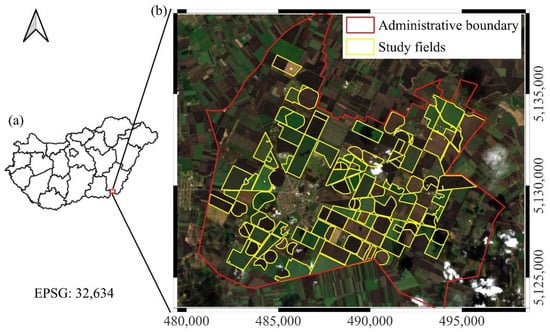
Figure 1.
An overview of the study site. (a) The location of the study area within Hungary; (b) the administrative boundary of Mezőhegyes and the investigated study fields, displayed on an EnMAP hyperspectral true color composite (acquired on 13 March 2025). Grid spacing represents 5 km intervals.
The dataset for this study was derived from 106 agricultural plots, representing a combined area of 5739 hectares. The crop composition within these selected fields reflects the estate’s diverse portfolio. While the area is particularly renowned for hybrid maize seed production, the studied parcels also encompass significant stands of winter wheat, winter barley, sunflower, alfalfa, and rapeseed, alongside maize cultivated for both silage and grain (fodder) purposes.
2.2. Hyperspectral Dataset
This study utilizes hyperspectral imageries acquired by the EnMAP satellite. Designed for high-fidelity Earth observation, the sensor covers the spectral range from 420 to 2450 nm across 224 contiguous bands, providing detailed spectral information in both the visible–near-infrared (VNIR) and shortwave infrared (SWIR) domains. The data feature a 30 m spatial resolution and a 30 km swath width, enabling the precise discrimination of surface materials and vegetation types.
For the 2025 growing season, three acquisitions (Table 1) were available for the study area—21 November 2024, 13 March 2025, and 10 August 2025 (Figure 2)—according to the authors’ proposal (Proposal No. A00001-P00875) to EnMAP. As EnMAP operates as a scientific mission with on-demand tasking capabilities rather than continuous global monitoring, the availability of cloud-free imagery for specific time windows is limited. Consequently, these three dates represent the only high-quality observations obtainable during the phenological cycle.

Table 1.
Detailed EnMAP acquisition parameters and atmospheric conditions for the study area.
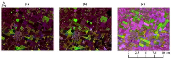
Figure 2.
False color composite ENMAP images (R: 1600 nm, G: 850 nm, B: 660 nm) acquired on (a) 21 November 2024, (b) 13 March 2025, and (c) 10 August 2025. Vegetation appears in green, while bare soil is shown in purple. The variation in purple tones reflects soil moisture: moist soil appears dark purple (November, March), whereas dry soil and stubble appear light purple (August).
EnMAP Level 2A products were processed through the official DLR Ground Segment using the PACO algorithm to physically compensate for atmospheric and geometric variations. This standardized procedure ensures that the acquisitions remain spectrally consistent and directly comparable despite varying off-nadir angles and solar positions. Such methodology guarantees the accuracy of the multi-temporal analysis and the scientific reproducibility of the study [30].
Regarding the preprocessing of the 13 March acquisition, we utilized the official EnMAP Quality Layer (QL) masks to identify clouds, shadows, and cirrus. To maintain data integrity, no training or validation samples were selected from these unsuitable areas. Furthermore, a spatial buffer zone was applied around all masked pixels to avoid fringe effects and ensure spectral purity. These steps ensured that the remaining clear pixels provided reliable and undisturbed coverage for the classification of winter crops.
2.3. Reference Data and Classification Strategy
2.3.1. Reference Data
The ground truth dataset was constructed using high-precision vector polygons representing the 106 investigated agricultural parcels (Figure 3). These geospatial data were obtained directly from the digital farm management system of the Nemzeti Ménesbirtok és Tangazdaság Zrt. A distinct advantage of this dataset is its reliability, as the parcel boundaries reflect official cadastral limits and the attribute data are derived from the estate’s actual sowing plans and harvest records. This authoritative source eliminates the uncertainty often associated with visual interpretation, ensuring spatially accurate and thematically correct reference labels for both training and validation.
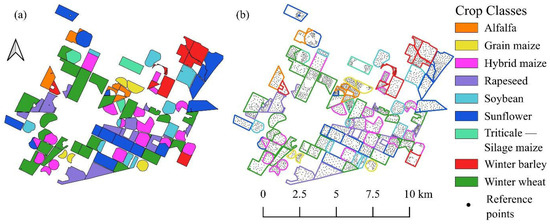
Figure 3.
Reference data used in study. (a) Seasonal crop map derived from official records (“Triticale–Silage Maize” indicates double cropping). (b) Visualization of sampling strategy showing ground truth points positioned within parcel interiors to avoid edge effects.
A manual sampling strategy was employed to generate the reference dataset (Figure 3). The sampling points were carefully positioned within the parcel interiors to strictly avoid edge effects and mixing with adjacent land cover types. To ensure the model’s robustness, the selection process aimed to capture the natural intra-field spectral variability of the crops; therefore, the dataset includes both spectrally homogeneous pixels and those exhibiting typical heterogeneity. However, pixels dominated by soil background noise or ambiguous spectral signatures (outliers) were explicitly excluded to maintain data quality. Crucially, labeling was performed in a multi-temporal manner: for each spatial sample point, the actual land cover class was recorded independently for all three acquisition dates, thereby capturing the complete phenological status and land use changes throughout the observed timeline. Finally, the reliability of the ground truth points was verified using high-resolution PlanetScope imagery and synchronized field surveys (Figure 4).
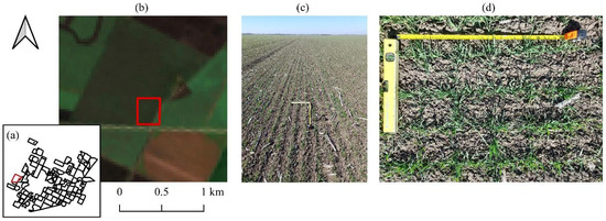
Figure 4.
Multiscale validation of winter wheat field (March 2025). (a) Location, (b) EnMAP satellite view, (c) landscape photo, and (d) nadir view with measuring tape. The red frame indicates the specific sampling location.
2.3.2. Classification Schemes
To assess the capabilities of the EnMAP hyperspectral imagery, two distinct classification strategies were employed based on the temporal characteristics of the vegetation. The first, a date-specific approach, was designed to reflect the instantaneous phenological status of the fields at each acquisition date. Since the spectral appearance of the landscape changes dynamically, class definitions were adjusted accordingly. For the November 2024 and March 2025 datasets, the analysis focused on active winter crops (winter wheat, winter barley, triticale, rapeseed) and perennials (alfalfa), while areas reserved for spring-sown crops were spectrally characterized as bare soil (Table 2). Conversely, in August 2025, the target shifted to summer crops (hybrid maize, grain maize, silage maize, sunflower, soybean, alfalfa); by this time, winter crops had been harvested, resulting in the reclassification of their locations as bare soil to represent stubble or tilled land.
Table 2.
The classification scheme and reference dataset statistics. The table indicates the presence of each crop type on the specific acquisition dates (Nov, Mar, Aug), the number of reference parcels, the total area in hectares, and the number of reference samples (pixels) selected for the modeling process.
Complementing the single-temporal analysis, a seasonal crop (multi-temporal) classification scheme was defined to map the dominant economic crop of the 2025 growing season. This approach integrates temporal information to eliminate the transient “bare soil” class inherent to the single-date assessments. In this scheme, every pixel is assigned to its primary crop type, regardless of whether it was harvested in early summer or autumn. The resulting thematic map encompasses the complete portfolio of cultivated species, including winter wheat, winter barley, triticale, rapeseed, hybrid maize, grain maize, silage maize, sunflower, soybean, and alfalfa.
2.3.3. Phenological Basis of Classification
The classification logic is grounded in the available hyperspectral time series, correlating the spectral reflectance properties with the specific development stages of the crops. The phenological status at the time of the three acquisitions was determined using the BBCH scale [31], as illustrated in Figure 5, and substantiated by the mean spectral profiles presented in Figure 6.
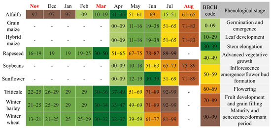
Figure 5.
The phenological calendar of the studied crops based on the BBCH scale. Colors indicate major growth stages, while the months highlighted in red correspond to the satellite image acquisition dates.
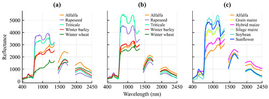
Figure 6.
Mean spectral reflectance profiles of classified crops for (a) 21 November 2024; (b) 13 March 2025; and (c) 10 August 2025.
The acquisition on 21 November 2024 coincides with the early vegetative phase of winter crops. At this stage, winter wheat, barley, rapeseed, and triticale (BBCH 19–25) exhibit active photosynthetic activity, resulting in a distinct vegetation signal (Figure 6a).
This allows for their spectral discrimination from parcels reserved for spring sowing, which are characterized by the reflectance features of bare soil or crop residues.
By the 13 March 2025 acquisition, winter crops had reached the stem elongation phase (BBCH 30–35). This stage is characterized by rapid biomass accumulation and canopy closure, providing strong green vegetation reflectance (Figure 6b). In contrast, the fields designated for summer crops (maize, sunflower, soybean) were in the seedbed preparation phase, where the spectral response is dominated by the soil background. This phenological divergence creates the maximum contrast between winter and summer cropping systems.
The 10 August 2025 image documents the phenological inversion of the landscape. Summer crops were in their reproductive or ripening stages (BBCH 65–80), showing high biomass and vigorous spectral reflectance. Conversely, winter crops had been harvested, presenting the spectral signature of dry stubble or plowed soil. Crucially, the timing of this acquisition enables the detection of double cropping: while standard cereal stubble is spectrally inactive, fields re-sown with silage maize show a renewed vegetative signal (BBCH 13–15), allowing for their identification based on active chlorophyll reflectance (Figure 6c).
2.4. Machine Learning and Deep Learning Implementation
The classification workflow was implemented in a high-performance Python 3.x environment using the TensorFlow 2.x deep learning framework (Keras API). Initial spatial processing and reference data preparation were conducted using QGIS 3.4 extended with the EnMapBox 3.16 plugin. Data standardization, performance metrics, and the baseline Random Forest classifiers were implemented using the Scikit-learn library. All experiments were executed in a GPU-accelerated environment to handle the computational load of the hyperspectral data cubes. To ensure the reproducibility of the results, a global deterministic seed (seed = 42) was applied to all random number generators prior to the training and validation procedures.
2.5. Single-Date Classification Models
To evaluate the spectral discriminative power of the EnMAP imagery at specific phenological stages, three distinct modeling approaches were applied independently to each acquisition date (November, March, and August).
2.5.1. Random Forest (RF)—Baseline
As a robust benchmark for shallow learning, a Random Forest classifier was implemented. The model processes the input as 1D spectral vectors (1 × 219) without considering spatial neighborhood information. The ensemble was configured with 500 decision trees to ensure higher stability compared to standard implementations. Trees were grown to their full depth using the Gini impurity criterion, and bootstrap sampling was enabled to improve generalization [32].
2.5.2. One-Dimensional Convolutional Neural Network (1D-CNN)
To assess the benefits of deep spectral feature extraction, a 1D-CNN was developed [33]. Unlike the RF, this model utilizes convolutional filters to learn hierarchical features directly from the continuous spectral curve. The architecture consists of a sequence of Conv1D layers (32 and 64 filters) with kernel sizes ranging from three to five, designed to capture local spectral absorption features. Each convolutional block is followed by Batch Normalization and ReLU activation, concluding with a dense layer for classification.
2.5.3. Dual-Stream Spatial–Spectral 2D CNN (DSS-2D)
The proposed DSS-2D architecture facilitates feature decoupling to address the high spectral redundancy of the 219 EnMAP bands. By separating the spatial and spectral streams, the model prevents the dominant spectral signal from overwhelming the extraction of subtle spatial textures. This ensures that morphological features and chemical signatures contribute non-redundantly to the final fusion layer. The network accepts 3D input patches of size 5 × 5 × 219 ( × × ) and processes them through two parallel, independent streams:
1. Spatial branch: This stream utilizes a standard 2D convolutional layer with 3 × 3 kernels (64 filters, padding = ‘same’). By operating on the local neighborhood, this branch is responsible for capturing texture features, edges, and inter-pixel spatial dependencies within the 5 × 5 window.
2. Spectral branch: This stream employs 1 × 1 point-wise convolutions (64 filters). This operation acts as a pixel-wise spectral feature extractor. It projects the high-dimensional spectral vector (219 bands) into a lower-dimensional feature space without mixing information from neighboring pixels, thereby preserving the purity of the spectral signature:
where
- : the output value of the feature map at spatial position (i, j) (scalar).
- : the non-linear activation function (ReLU).
- : the bias term (scalar).
- : the index of the input channel (ranging from 1 to ).
- : the spatial indices of the kernel relative to the center position (ranging from −[/2] to [/2]).
- : the number of input channels.
- : the learnable weights of the kernel .
- : the input feature map value at a given position .
- : the kernel spatial dimension, where = 3 for the spatial branch (capturing local texture and neighborhood context) and = 1 for the spectral branch (performing pixel-wise spectral feature extraction).
Both branches utilize BN and the ReLU activation function. The feature maps from the spatial and spectral streams are then concatenated along the channel dimension. To prevent overfitting and reduce the total number of parameters, the fused features are spatially compressed using Global Average Pooling (GAP), which transforms the 5 × 5 feature maps into a 1D vector. This vector is fed into a fully connected dense layer with 256 neurons (followed by a dropout of 0.5) to learn high-level non-linear combinations. Finally, a Softmax output layer produces the class probabilities (Table 3).
2.6. Multi-Temporal Seasonal Classification Models
To evaluate the added value of temporal information, a second set of models was developed to perform classification using the full seasonal time series (November, March, August) simultaneously.
2.6.1. Multi-Temporal Random Forest (Seasonal RF)
A baseline multi-temporal classifier was implemented by extending the Random Forest approach. The spectral bands from all three acquisition dates were stacked into a single feature vector (3 × 219 = 657 features per pixel). The model hyperparameters (500 trees) were kept identical to the single-date RF to ensure a direct comparison of the temporal integration effect.
2.6.2. 3D-ResNet with Squeeze-And-Excitation (3D-SE-ResNet)
To fully leverage the complex spatio-temporal structure of the EnMAP data, a 3D Convolutional Neural Network was designed. Unlike the 2D approach, this architecture treats the time series as the third dimension of the input volume, processing 4D patches of size 3 × 5 × 5 × 219 (time × height × width × bands) (Table 3). The backbone is based on the ResNet architecture adapted for 3D data, where the fundamental operation is 3D convolution [34]. This allows the model to simultaneously capture local spatial interactions and temporal evolution:
Table 3.
A summary of the baseline and deep learning models, including input shapes and architectural specifications, used in this study.
Table 3.
A summary of the baseline and deep learning models, including input shapes and architectural specifications, used in this study.
| Model Name | Type | Input Shape (H × W × C) | Architecture Details |
|---|---|---|---|
| RF | Baseline (Shallow) | 1 × 219 | Ensemble of 500 trees; Gini impurity; bootstrap sampling enabled. No spatial context. |
| Seasonal RF | Baseline (Multi-Temporal) | 1 × 657 | Stacked input of 3 dates (3 × 219 bands). Same configuration as single-date RF (500 trees). |
| 1D-CNN | Deep Learning (Spectral) | 1 × 219 × 1 | 3 distinct Conv1D layers (filters: 32, 64); kernel sizes: 3–5; batch normalization + ReLU; MaxPooling1D. |
| DSS-2D | Deep Learning (Spatial–Spectral) | 5 × 5 × 219 | Dual-Stream Architecture: |
| |||
| |||
| |||
| 3D-SE-ResNet | Deep Learning (Spatio-Temporal) | 3 × 5 × 5 × 219 | 3D-CNN Backbone: |
| |||
| |||
|
To prevent gradient vanishing and enable deeper feature extraction, identity shortcuts (residual connections) are employed. The output of residual block is defined as the summation of the input and the learned residual mapping:
To address the high inter-band correlation and spectral redundancy inherent in EnMAP data, Squeeze-and-Excitation (SE) blocks were integrated within the residual units. Unlike standard CNNs that treat all channels with equal importance, this mechanism allows for the explicit modeling of the complex interdependencies between over 200 spectral bands and multi-temporal phases. The SE block adaptively recalibrates channel-wise feature responses by “weighting” the most discriminative spectral regions while suppressing less informative or noisy channels. This process is executed in two primary steps: Squeeze (global spatial information compression) and Excitation (adaptive channel-wise weighting):
where
- : the output value at spatial position (i, j) and temporal index t (scalar).
- : the temporal kernel depth .
- : the residual mapping function.
- : the input and output tensors of the residual block, with shape .
- : the global average statistic for the c-th channel.
- : the feature map before recalibration, with shape .
- : the final recalibrated feature map (scalar).
- : the learnable weights of the SE block.
- : the number of input channels (219 bands).
2.7. Training Protocol
All deep learning models (1D-CNN, DSS-2D, and 3D-SE-ResNet) were trained using a unified protocol (Table 4). The Adam optimizer was employed with an adaptive learning rate initialized at 1 × 10⁻⁴. The Sparse Categorical Cross-entropy served as the loss function. Models were trained for 40 to 60 epochs with a batch size of 16 or 32, depending on the memory requirements of the architecture. An Early Stopping mechanism was implemented (patience = 8–12 epochs), which terminated training if the validation loss ceased to improve, automatically restoring the best model weights.
Table 4.
Hyperparameter settings and training configuration employed for deep learning models.
2.8. Validation
To address the high spatial autocorrelation of agricultural imagery and prevent data leakage, a strict spatial field-based splitting strategy was implemented. Unlike standard random sampling, this approach assigns all pixels within a specific agricultural parcel exclusively to the same partition, ensuring the complete spatial independence of the testing set within the proposed framework.
The evaluation followed a repeated stratified k-fold scenario, consisting of 5 spatial splits, each repeated 5 times with different initialization seeds (totaling 25 independent runs) (Figure 7). To ensure rigorous comparability, all single-date models were evaluated on identical cross-validation splits. Similarly, the multi-temporal models shared a consistent set of partitions, which were distinct from the single-date splits. In every iteration, after assigning fields to the test partition, exactly 50 samples per class were randomly selected from these current test fields to form the final balanced evaluation set.
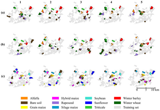
Figure 7.
The spatial distribution of training (gray) and testing (colored) samples across the five random scenarios (columns 1–5) and three datasets: (a) November, (b) March, and (c) August. Due to the limited availability of parcels in certain minority crop classes, some specific fields appear in the test set across multiple splits to ensure adequate representation.
For each run, feature standardization was fit solely on the training data to prevent leakage, and geometrical augmentation (random rotations) was applied to the training patches. During the optimization phase, the training data were further divided into an 80:20 ratio, where 20% of the samples served as an internal validation set to monitor performance and trigger Early Stopping.
Accuracy Assessment Metrics
To quantitatively assess classification performance, standard accuracy metrics were derived from the population error matrix of size × , where represents the number of crop classes. The diagonal elements indicate the number of correctly classified samples for class , while off-diagonal elements represent misclassifications. The overall accuracy (OA) was calculated to represent the proportion of correctly classified samples relative to the total number of evaluated samples:
where is the total number of test samples. While OA provides a global performance measure, it may not fully reflect the model’s ability to distinguish individual crop types, particularly in imbalanced scenarios. Therefore, the Producer’s Accuracy (PA) (Recall) and User’s Accuracy (UA) (Precision) were computed for each class to quantify omission and commission errors, respectively:
where denotes the total number of ground truth samples for class (column total), and represents the total number of samples predicted as class (row total). In the Results Section, the False Discovery Rate (FDR) is also reported to explicitly highlight commission errors ).
The F1-Score, defined as the harmonic mean of PA and UA, was employed to evaluate the classification performance for each individual crop class:
For the multi-temporal model comparison, the Macro-averaged F1-Score was used to ensure that all classes contribute equally to the final score, regardless of sample size variations in the training set.
3. Results
3.1. Performance of Single-Date Classification Models
3.1.1. Efficiency Assessment of Single-Date Classification
This study addresses the critical operational challenge of single-date mapping, determining the immediate land cover status at specific phenological moments without reliance on full temporal sequences. The primary objective of this experimental phase was to evaluate how effectively the proposed DSS-2D architecture can extract identifying features from a single observation. This capability offers a “real-time” alternative to retrospective seasonal monitoring.
The comparative analysis demonstrates that the DSS-2D model provides a highly reliable solution for snapshot classification, as it consistently outperforms both the RF baseline and the spectral-only 1D-CNN across all acquisition dates. Pixel-based methods proved highly sensitive to the lack of temporal context and struggled to resolve spectral ambiguities in both early and late phenological stages. In contrast, the DSS-2D model successfully compensated for this limitation by integrating spatial texture features.
Regarding the algorithmic stability, the proposed method exhibited remarkable robustness across the 25 independent experimental runs. The standard deviation of the OA remained below 2.0% for the acquisitions with developed canopy cover, specifically ±1.4% in March and ±1.9% in August. In the early vegetative phase for autumn-seeded crops (November), the deviation was slightly higher (±2.9%). This increased variability reflects the inherent difficulty of detecting sparse vegetation signals against a dominant soil background, yet it remains significantly lower than the volatility observed in the 1D-CNN baseline (e.g., ±6.2% in August).
3.1.2. November Acquisition (Early Vegetative Phase)
The November acquisition (BBCH 13–21) served to test the ability of the models to identify crops during the early emergence phase. At this stage, the spectral signal is overwhelmingly dominated by the soil background. Winter crops have a low LAI and are spectrally similar to bare soil or stubble fields. This ambiguity caused the pixel-based 1D-CNN to struggle significantly, and it achieved a Recall of only 74.8% for the winter wheat class. Although the RF baseline proved more resilient to this spectral mixing, with a Recall of 84.8%, it still failed to match the detection capability of the proposed method. This comparison highlights the limitations of pure spectral monitoring in the early season, which often leads to a systematic underestimation of the cultivated area.
The DSS-2D model successfully mitigated this issue by leveraging the spatial branch of its architecture. Even in the absence of a closed canopy, the convolutional layers effectively detected the faint, periodic row structures and tillage patterns characteristic of emerging vegetation. Consequently, the model improved the winter wheat Recall to 86.1% and achieved a global OA of 97.2% (Table 5). Furthermore, for silage maize, which is present as stubble or bare soil at this time, the model maintained an FDR of just 0.5%. These results confirm that for operational tasks requiring early-season mapping, spatial features provide discriminative information that spectral data alone cannot supply.
Table 5.
Performance assessment of single-date models across distinct phenological phases. The table summarizes the overall accuracy (OA) and the specific detection capability (Recall, FDR) for the critical classes.
3.1.3. March Acquisition (Stem Elongation and Canopy Closure)
The March acquisition (BBCH 30–39) represented the active vegetative phase where winter crops reached stem elongation and maximum canopy closure. The challenge here shifted from background noise to the spectral similarity between biologically related species. The RF baseline struggled to differentiate winter barley from winter wheat and achieved a Recall of 83.6% for the barley class. The spectral signatures of these two cereals are nearly identical in the visible and near-infrared domains during this intensive vegetative phase, leading to “salt-and-pepper” noise in the pixel-based classification maps.
The DSS-2D model resolved this ambiguity entirely and achieved a near-perfect OA of 99.2%. Error decomposition analysis revealed an allocation disagreement of 0.0%, implying that the model made virtually no spatial errors in boundary detection. Specifically, it achieved an FDR of 0.0% and 96.3% Recall for winter barley. This demonstrates that at this phenological stage, the distinct canopy textures of barley and wheat allow for their precise separation. These textural differences are likely related to variations in sowing density and leaf orientation, making the March acquisition an optimal window for differentiating winter cereals using spatial–spectral methods.
3.1.4. August Acquisition (Reproductive Phase and Maturity)
The August acquisition (BBCH 70–89) tested the models on the most taxonomically complex task. This involved separating fully developed maize varieties, including silage maize, grain maize, and hybrid maize, during the peak growing season (Figure 8). These crops share almost identical spectral traits but differ in agronomic management and canopy architecture, such as planting density and tassel distribution. Standard spectral classifiers failed to reliably distinguish these crops. The RF model yielded an FDR of 12.3% for silage maize, meaning that more than one in ten pixels classified as silage maize was incorrect.
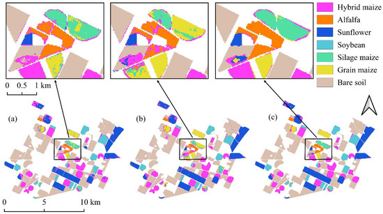
Figure 8.
Classification maps derived from the August imagery: (a) Random Forest; (b) 1D-CNN; (c) DSS-2D.
In strong contrast, the DSS-2D model demonstrated the decisive advantage of spatial–spectral learning. It achieved a global OA of 98.9% and reduced the FDR for silage maize to a negligible 1.9%. This performance leap, which reduced the error rate by a factor of six compared to the baseline, confirms that the convolutional features successfully encoded the textural differences associated with crop height and structure. The results prove that accurate discrimination of agronomically distinct but spectrally similar varieties is achievable with single-date imagery, provided that spatial context is adequately modeled.
3.1.5. Ablation and Comparative Analysis of Single-Date Models
Using the August acquisition as a representative case for high taxonomic complexity, the ablation analysis reveals a distinct performance hierarchy between the evaluated models (Figure 9). Traditional classifiers (RF, 1D-CNN) and the generic 2D-CNN baseline (92.2% OA) were significantly outperformed by the specialized branches, confirming that isolating spectral and spatial features is more effective for high-dimensional hyperspectral data than the integrated “all-in-one” approach of standard 2D-CNNs. Regarding training data sensitivity, DSS-2D demonstrated exceptional stability; while the performance of the RF and 1D-CNN models declined sharply at lower sampling densities, the proposed architecture maintained an OA above 95% even at a 0.25 training ratio. The peak performance of 99.3% OA achieved by the full DSS-2D model confirms the synergy of the dual-stream approach, where diagnostic spectral identification is reinforced by spatial structural extraction, ensuring high precision even under minimal sampling conditions.
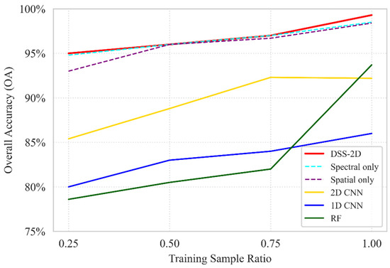
Figure 9.
An ablation study of the baseline RF, 1D CNN, standard 2D CNN, and DSS-2D models and the separated spectral and spatial branches (dashed) under different training data ratios based on OA.
3.2. Multi-Temporal Classification Results
3.2.1. Global Accuracy Assessment
Classification performance of the multi-temporal models was evaluated using the complete three-date EnMAP dataset to determine the efficacy of deep learning in handling high-dimensional spectral time series. The proposed 3D-SE-ResNet model achieved an overall accuracy (OA) of 92.9%, demonstrating a substantial improvement over the Seasonal RF baseline, which achieved 84.5% (Table 6). This performance gap highlights the limitations of traditional machine learning when applied to hyperspectral data cubes. The Seasonal RF, processing a stacked feature vector of 657 variables, exhibited signs of the “curse of dimensionality”, where the high correlation between contiguous spectral bands introduced significant spectral redundancy, hampering the classifier’s generalization capability. Disagreement metrics further validate 3D-SE-ResNet’s superiority: it reduced allocation disagreement from 4.8% (RF) to 0.74%, ensuring high spatial consistency and parcel boundary precision while eliminating pixel-level noise. Quantity disagreement also dropped from 10.67% to 6.37%, improving total area estimation reliability. In contrast, 3D-SE-ResNet effectively utilized the spatio-temporal volume, with the Squeeze-and-Excitation mechanisms successfully prioritizing relevant spectral channels while suppressing noise.
Table 6.
Multi-temporal classification performance. Comparison of global overall accuracy and class-specific metrics (Recall, FDR) for the Seasonal RF baseline and the 3D-SE-ResNet model.
3.2.2. Class-Specific Evaluation
The superiority of the deep learning architecture is most pronounced in crops with distinct but complex phenological trajectories. For silage maize, the 3D-SE-ResNet achieved a near-perfect Recall of 99.6%, whereas the Seasonal RF reached only 90.7%. The contrast was even sharper for soybean, where the baseline struggled with severe confusion, resulting in a critically high FDR of 17.9%. This means that nearly one in five pixels classified as soybean by the Seasonal RF was incorrect. The deep model reduced this error rate to a negligible 2.8%, accurately capturing the rapid vegetative development characteristic of broad-leaved summer crops.
Confusion matrix analysis indicates that spectral overlap between hybrid maize and rapeseed during senescence presented the greatest challenge for both models. However, 3D-SE-ResNet achieved 928 correct hits for hybrid maize, significantly outperforming the Seasonal RF, which managed only 166. The 3D network, aided by the Squeeze-and-Excitation mechanism, successfully distinguished subtle spectral trajectories between dry stubble and drying crop stands.
Furthermore, the analysis of winter barley provides insight into the models’ handling of “presence–absence” temporal patterns, as the crop is already harvested by the August acquisition. The Seasonal RF failed to robustly model this transition, resulting in a low Recall of 78.6%. The 3D-SE-ResNet model, however, effectively encoded the senescence and harvest signal, achieving a Recall of 98.4%. This confirms that the spatio-temporal filters can adaptively learn diverse phenological profiles, distinguishing between active vegetation and stubble within the same growing season better than the stacked-vector approach.
3.2.3. Ablation and Comparative Analysis of Multi-Temporal Models
The robustness of the proposed 3D-SE-RESNET model was further evaluated by comparing it against the baseline Seasonal RF and the 3D-RESNET ablation variant (defined as the model architecture without the Squeeze-and-Excitation module). As illustrated in Figure 10, the results underscore the superior data efficiency of the 3D-SE-RESNET architecture, which achieves an OA of 84.6% at the lowest sampling density, a performance level nearly identical to that of the Seasonal RF at its full training capacity 84.5%. This confirms that the proposed deep learning framework effectively extracts diagnostic spatio-temporal features even when ground truth data are minimal. The ablation study highlights the critical contribution of the SE mechanism to the model’s stability. At a 0.25 ratio, the inclusion of SE blocks provides a 3.3% absolute gain in accuracy compared with the standard 3D-RESNET model without the attention module, demonstrating its ability to dynamically recalibrate spectral–temporal feature maps under high-uncertainty conditions. While the performance gap between the 3D-based models narrows at intermediate sampling stages, the 3D-SE-RESNET maintains its dominance at full capacity, reaching a peak OA of 93.0%. This represents a 2.0% improvement over the non-SE 3D-RESNET variant and an 8.5% lead over the RF baseline, validating that the synergistic combination of 3D convolutions and attention mechanisms is essential for capturing the complex phenological signatures in multi-temporal hyperspectral datasets.
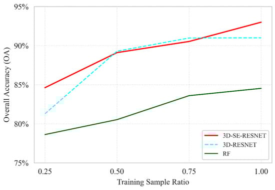
Figure 10.
Ablation study comparing the proposed 3D-SE-RESNET with the baseline Seasonal RF and the 3D-RESNET variant (without SE blocks, indicated by dashed lines) evaluated under different training data ratios based on OA.
3.3. Relationship Between Spectral Importance and Biophysical Development
The dynamic shift in feature importance across the growing season confirms that the decision boundaries are governed by the transition from soil-dominated to vegetation-dominated signals. The model tracks key biophysical parameters that characterize each phenological stage by leveraging specific EnMAP bands.
In the November acquisition, the combined importance of SWIR II (30.1%) and SWIR III (10.9%) accounts for 41% of the decision weight (Figure 11). This high significance is a direct consequence of the sparse canopy cover typical of winter cereals during early establishment. At this stage, the classification is primarily driven by soil moisture and organic matter content, which are sensed through the specific absorption properties of the long-wave infrared spectrum. This reliance on soil–background contrast allows the model to differentiate fields even when the winter wheat and barley are only in the initial leaf development phase.
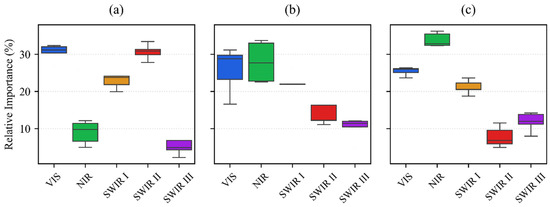
Figure 11.
The relative importance of spectral regions for crop classification at three distinct phenological stages using the DSS-2D model and EnMAP hyperspectral data: (a) November; (b) March; (c) August. The spectral bands are VIS (400–700 nm), NIR (700–1000 nm), SWIR I (900–1390 nm), SWIR II (1480–1760 nm), and SWIR III (1950–2450 nm). The boxplots illustrate the distribution of feature importance across 25 model iterations, where the horizontal black line denotes the median and the box represents the interquartile range.
In the March image, the model reallocates its attention toward the VIS (34.6%) and NIR (26.1%) regions, which together account for 60.7% of the total importance. This shift corresponds to the rapid increase in chlorophyll concentration and above-ground biomass during the stem elongation phase. The peak significance of the VIS spectrum indicates that the model distinguishes winter wheat from winter barley based on subtle variations in pigment composition and nitrogen uptake. Simultaneously, the increased NIR contribution reflects the development of the leaf cellular structure, which serves as a proxy for canopy density and vigor as the crops move toward their peak vegetative state.
In the August dataset, the hyperspectral SWIR I (18.8%) range becomes particularly critical. As summer crops reach maturity and senescence begins, the model monitors the water-to-dry-matter ratio within the plant tissues. The NIR importance of 27.5% is coupled with SWIR I signals to track changes in leaf dry matter, cellulose, and lignin content. For maize varieties, this transition zone is essential for detecting the onset of grain hardening and dry down. The fact that SWIR III importance reaches its minimum of 7.7% during this period confirms that the model effectively ignores soil background noise when the water-rich, dense vegetation is at its physiological peak.
The temporal progression from soil mineralogy in November to pigment and biomass in March and finally to dry matter and structure in August validates that the classification is driven by actual physiological changes. The results prove that the model successfully internalizes the seasonal physics of the agricultural landscape to ensure robust performance across diverse crop types.
For the three-date 3D-SE-ResNet model, the importance of the spectral ranges was as follows: the NIR range was the most influential with 24.1%, followed by the VIS (21.9%) and SWIR III (20.7 percent) regions. The SWIR II (17%) and SWIR I (16%) ranges also contributed significantly to the model’s performance, confirming the effective utilization of the diagnostic bands available in hyperspectral data.
3.4. Computational Efficiency and Training Convergence
The assessment of computational efficiency reveals the strategic value of the proposed architectures in handling the high-dimensional complexity of multi-temporal EnMAP data (Figure 12). To provide a standardized comparison, training times were measured for the full construction of the Seasonal RF model and for 10 training epochs for the deep learning architectures.
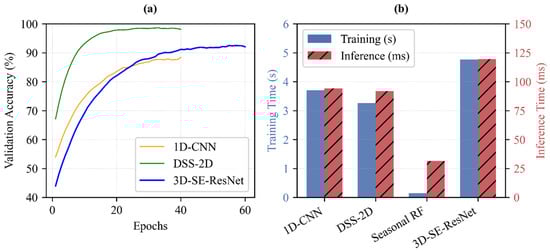
Figure 12.
Assessment of model efficiency. (a) Mean validation accuracy curves showing training convergence. (b) Comparison of average training times totaling 10 epochs (blue bars, left axis) and inference times per sample (red bars, right axis). Results are based on 25 independent runs (5-fold spatial cross-validation with 5 repetitions). All benchmarks were conducted on workstation equipped with Intel Core i7-14700F CPU, 32 GB RAM, and NVIDIA GeForce RTX 4060 Ti (8 GB) GPU.
In single-date scenarios, the proposed DSS-2D model (training: 3.26 s; inference: 0.09 s) proves superior to the 1D CNN baseline (training: 3.71 s; inference: 0.09 s) by delivering improved time efficiency in both training and prediction cycles (Figure 12b). For multi-temporal analysis, which integrates 219 spectral bands across three phenological stages, the trade-off between computational cost and classification quality becomes critical.
While the seasonal RF is exceptionally fast to train (total training: 0.14 s; inference: 0.03 s), it cannot model the intricate temporal dynamics with the same precision as 3D-SE-ResNet. The results confirm that the additional training time required for 3D-SE-ResNet (training: 4.76 s per 10 epochs; inference: 0.12 s) is a necessary investment for the resulting accuracy gains. As shown in the convergence curves (Figure 12a), the structural complexity of the 3D architecture, including its Squeeze-and-Excitation (SE) blocks, allows for more robust feature extraction from the EnMAP cubes.
4. Discussion
The primary objective of this study was to evaluate the suitability of EnMAP hyperspectral imagery for agricultural mapping in an intensive production environment. The results confirm our working hypotheses regarding the superiority of spatial–spectral deep learning and the critical role of the SWIR domain. This section interprets the findings in the context of algorithmic performance, spectral discriminability, and operational feasibility under data-constrained conditions.
4.1. Superiority of Spatial–Spectral Deep Learning over Pixel-Based Methods
Our first hypothesis posited that CNNs would outperform traditional baseline models. The results strongly corroborate the consistently higher accuracy of the DSS-2D model (OA > 97%) compared with the RF and 1D-CNN baselines across all acquisition dates.
The failure of the 1D-CNN to surpass even the RF baseline in certain scenarios offers a critical insight into the relationship between model architecture and sample size. Deep learning models typically require vast amounts of labeled data to generalize effectively. In our study, the training dataset was inherently limited. The 1D-CNN, relying solely on spectral vectors, lacked the capacity to generate sufficient feature variance from the limited samples, leading to overfitting and sensitivity to spectral noise.
In contrast, the success of the DSS-2D architecture can be attributed to its ability to exploit spatial context and data augmentation. Crucially, the explicit separation of the spatial and spectral branches prevents the high-dimensional spectral data (219 bands) from overwhelming the spatial feature extraction process. In a standard joint CNN, the dominant spectral correlations often suppress the learning of subtle spatial patterns, such as crop row textures. By disentangling these streams, our dual-stream approach ensures robust learning of both domains. By processing 5 × 5 patches, the model learned textural features, such as row spacing and canopy roughness, which are more robust against intra-class spectral variability than raw reflectance values. Furthermore, our ablation experiments explicitly verified the independent contributions of both the spatial and spectral branches. The results demonstrated that while the spectral branch is essential for capturing baseline biochemical traits, the spatial branch is indispensable for resolving intra-class variances and boundary pixels. Furthermore, the 2D nature of the input allowed for geometrical augmentation, effectively multiplying the training variance without requiring additional ground truth collection. To further validate the robustness of this architecture under data-constrained conditions, our sensitivity analysis across different training sample ratios (from 25% to 100%) confirmed that the proposed models maintain exceptionally high performance even with significantly reduced training datasets. This confirms that for operational mapping with limited reference data, integrating spatial dimensions is not merely an accuracy booster but a prerequisite for the stable convergence of deep learning models.
4.2. The Critical Role of the SWIR Domain (1000–2450 nm)
The feature importance analysis validates the hypothesis that the extended spectral range of EnMAP provides identifying information that standard multispectral sensors cannot fully capture. While visible and NIR bands drove the classification during the peak vegetative stage, the SWIR ranges proved indispensable during the early and late phenological phases.
Specifically, the high contribution of SWIRs II and III in November highlights the importance of characterizing soil background properties, including moisture and organic matter, to differentiate sparse winter crops from bare soil. Similarly, the dominance of SWIR I in August confirms that monitoring ligno-cellulose content and crop water stress is essential for separating spectrally similar maize varieties during senescence. These findings underscore that for accurate crop monitoring outside the peak greenness window, the 1000–2450 nm spectral domain is a decisive factor, justifying the use of hyperspectral sensors over cheaper multispectral alternatives.
4.3. Seasonal Mapping with Sparse Temporal Sampling
A key operational question was whether a seasonal land cover map could be derived from a limited number of hyperspectral acquisitions, as opposed to the dense time series required by multispectral approaches. Our results demonstrate that 3D-SE-ResNet achieved a high overall accuracy (92.9%) using only three images.
This challenges the prevailing paradigm that high temporal resolution is strictly necessary for crop classification. The Seasonal RF baseline struggled with the “curse of dimensionality” when stacking highly correlated bands, which diluted the temporal signal. However, the 3D deep learning model successfully compensated for the temporal sparsity by leveraging the extreme spectral depth of the EnMAP data. The necessity of this complex architecture was validated through our ablation studies, which confirmed that both the 3D convolutions and the SE module are critical for performance. The Squeeze-and-Excitation mechanism played a pivotal role here, allowing the model to adaptively focus on the most relevant spectral features for each timestamp. This suggests that spectral resolution can effectively substitute for temporal frequency, enabling accurate seasonal mapping even in cloud-prone regions where continuous monitoring is not feasible.
These findings are consistent with our previous research in the same study area (Mezőhegyes, Hungary). We have empirically demonstrated that limited temporal sampling can be effectively compensated for by high spectral and spatial depth; for instance, using only two DESIS acquisitions (VNIR range) paired with a Wavelet-attention CNN, an OA of 97.89% was achieved [35]. Furthermore, by fusing sparse hyperspectral data (three acquisitions) with LiDAR-derived morphological features, a top OA of 98.86% was recorded [36]. While those earlier studies reported higher overall accuracies, it is important to note that they categorized a more limited number of crop types. The present study proves that the inclusion of the SWIR domain (1000–2500 nm) provides an even more robust discriminative signal. This confirms that for operational monitoring, spectral resolution can effectively substitute for temporal frequency, enabling accurate seasonal mapping even in cloud-prone regions where continuous monitoring is not feasible.
4.4. Computational Efficiency
While the 3D-SE-ResNet model requires higher computational resources during the training phase compared to traditional baselines such as the RF, our evaluation on modern hardware confirms this is a justified one-time investment. The operational inference time remains highly efficient (approx. 0.12 s), making it completely suitable for large-scale processing without creating a bottleneck. The increased computational overhead is vastly outweighed by the value of the improved classification accuracy. In precision agriculture, accurate crop identification is the fundamental baseline for high-stakes, cost-intensive interventions such as fertilization, irrigation, and plant protection. A highly precise crop map minimizes the misallocation of these expensive agricultural inputs, ensuring that the initial computational cost translates directly into significant economic savings.
4.5. Limitations and Future Directions
This study serves as a crucial proof-of-concept for the DSS-2D and 3D-SE-ResNet architectures, utilizing 106 high-quality ground-verified plots to establish a scalable methodological baseline. While spatial smoothing through 2D and 3D convolutions is highly advantageous for the large, homogeneous parcels investigated here, future research must evaluate model transferability to fragmented smallholder landscapes. In such heterogeneous environments, EnMAP’s 30 m spatial resolution often leads to significant mixed-pixel effects at field boundaries. To address these artifacts and improve classification granularity, future architectural optimization should prioritize the integration of sub-pixel unmixing, deep learning-based super-resolution methods, or higher-resolution auxiliary data.
The reliance on a single growing season and a specific geographic footprint limits the current assessment of inter-annual and regional generalization. Agricultural cycles are subject to significant year-to-year variability driven by climatic fluctuations and shifting management practices. Future research will prioritize incorporating domain adaptation and transfer learning techniques to mitigate the spectral shifts caused by varying phenological timings, thereby reducing the intensive requirement for annual ground truth collection. During our experiments, we also evaluated the highly prominent Vision Transformer (ViT) architecture. However, due to the inherent data-hungry nature of transformers, the model suffered from overfitting and underperformed compared to the proposed CNN-based architectures when restricted to our specific multi-temporal sample size. Notably, as larger-scale geographical coverage and multi-year datasets become available, the implementation of these more complex ViT architectures will become viable. These models could eventually leverage their superior global attention mechanisms to capture even more intricate spatial–spectral dependencies across diverse landscapes. To support these advanced algorithmic developments, future efforts will also aim to establish the comprehensive ground truth and hyperspectral archive of the Mezőhegyes study area as an open-access benchmark dataset for the remote sensing community.
A significant limitation of the current study stems from the experimental, tasking-based nature of the EnMAP mission, where critical phenological transitions and the peak vegetative stages (May–July) were not captured due to limited on-demand observation capacity. The absence of data during this optimal window is disadvantageous, as it restricts the model’s ability to observe maximum canopy development and specific flowering traits that are highly diagnostic for crop differentiation. However, the high accuracy achieved despite this temporal sparsity is highly encouraging for the development of real-time operational monitoring systems. The ultimate value of the proposed architectures lies in their potential deployment within cloud-based infrastructures, such as the Copernicus Data Space Ecosystem. This transition toward automated processing pipelines is expected to be catalyzed by the upcoming Copernicus CHIME mission [37], which will provide systematic, high-frequency hyperspectral revisit capabilities. Integrating these deep learning architectures into next-generation frameworks will transform hyperspectral data from specialized research outputs into actionable decision support tools for precision agriculture and large-scale food security monitoring.
5. Conclusions
This study provided a comprehensive evaluation of EnMAP hyperspectral imagery for agricultural land cover mapping, demonstrating that deep spectral–spatial feature extraction can effectively overcome the limitations of data sparsity. Our findings lead to three primary conclusions regarding the operational implementation of spaceborne imaging spectroscopy.
First, the integration of spatial context is a prerequisite for robust hyperspectral classification when training data are limited. The comparative analysis revealed that pixel-based methods, including 1D-CNN and RF, are susceptible to overfitting and spectral noise. In contrast, the proposed DSS-2D and 3D-SE-ResNet architectures successfully exploited texture and pattern recognition. Supported by comprehensive ablation and sensitivity analyses, these models demonstrated high stability (OA > 97%) even with significantly restricted ground truth datasets. This confirms that treating hyperspectral data as a spatial–spectral volume rather than a 1D vector is critical for algorithmic convergence.
Second, this study validates the distinct biophysical value of the full 420–2450 nm spectral range. While standard multispectral sensors are sufficient for monitoring peak greenness, the SWIR domain proved indispensable for differentiating crops during critical phenological transitions. Specifically, the SWIR bands were essential for characterizing soil background properties in the early season and identifying senescence markers in the late season. This suggests that future agricultural monitoring systems must prioritize the inclusion of the 1000–2450 nm range to resolve spectral ambiguities between biologically similar crop types, which is a fundamental requirement for optimizing cost-intensive precision agriculture practices, such as variable-rate fertilization and targeted irrigation.
Finally, we demonstrated that high spectral resolution can effectively compensate for low temporal frequency. Even with the sparse availability of EnMAP acquisitions and the complete absence of data during the peak vegetative stages, the 3D deep learning model successfully reconstructed the seasonal crop map with an accuracy of 92.9%. This finding has significant implications for the upcoming Copernicus CHIME mission. It serves as a proof-of-concept that once the systematic revisit capability of CHIME is combined with the deep learning architectures proposed herein, it will be feasible to deliver continuous, high-precision agricultural services on a continental scale, transcending the current limitations of experimental tasking missions.
Author Contributions
Conceptualization, L.M., Z.T. and J.S.; methodology, L.M. and M.S.; software, M.S.; validation, M.S. and J.S.; formal analysis, L.M. and M.S.; investigation, M.S., J.M. and E.S.J.; resources, L.M. and J.M.; data curation, M.S., D.V.-S. and D.L.-K.; writing—original draft preparation, M.S.; writing—review and editing, L.M.; visualization, M.S. and Z.T.; supervision, L.M.; project administration, L.M.; funding acquisition, L.M. All authors have read and agreed to the published version of the manuscript.
Funding
This research was funded by the NKFIH-National Research and Innovation Office (NKFIH ADVANCED), grant no. 149686. Project title: Definition and Geospatial Big Data Analysis of Spectral Fingerprints of Healthy and Unhealthy Crops Using Fused Hyperspectral Multi-temporal Satellite and Field Remotely Sensed Data and Deep Learning Methods.
Data Availability Statement
The ENMAP images were acquired according to the accepted scientific proposal of Laszlo Mucsi (Proposal No. A00001-P00875). All used ENMAP images available for download at the EOC Geoservice are accessible using a unified Geoservice Account. The agricultural reference data are owned by Mezőhegyesi Ménesbirtok Zrt.
Acknowledgments
The authors would like to thank Mezőhegyesi Ménesbirtok Zrt. for providing the agricultural reference data used in this study.
Conflicts of Interest
Author Dorottya Litkey-Kovács was employed by the company Lajtamag Ltd. The remaining authors declare that the research was conducted in the absence of any commercial or financial relationships that could be construed as a potential conflict of interest.
Abbreviations
| 1D-CNN | 1D Convolutional Neural Network |
| BN | Batch Normalization |
| DSS-2D | Dual-Stream Spatial-Spectral 2D CNN |
| EnMAP | Environmental Mapping and Analysis Program |
| FDR | False Discovery Rate |
| GAP | Global Average Pooling |
| LAI | Leaf Area Index |
| NIR | Near-Infrared |
| OA | Overall Accuracy |
| PA | Producer’s Accuracy |
| ReLU | Rectified Linear Unit |
| RF | Random Forest |
| SE | Squeeze-and-Excitation |
| SWIR | Shortwave Infrared |
| UA | User’s Accuracy |
References
- Buchhorn, M.; Lesiv, M.; Tsendbazar, N.-E.; Herold, M.; Bertels, L.; Smets, B. Copernicus global land cover layers-collection 2. Remote Sens. 2020, 12, 1044. [Google Scholar] [CrossRef]
- Bolton, D.K.; Gray, J.M.; Melaas, E.K.; Moon, M.; Eklundh, L.; Friedl, M.A. Continental-scale land surface phenology from harmonized Landsat 8 and Sentinel-2 imagery. Remote Sens. Environ. 2020, 240, 111685. [Google Scholar] [CrossRef]
- Clevers, J.G.P.W.; Gitelson, A.A. Remote estimation of crop and grass chlorophyll and nitrogen content using red-edge bands on Sentinel-2 and -3. Int. J. Appl. Earth Obs. Geoinf. 2013, 23, 344–351. [Google Scholar] [CrossRef]
- Homolová, L.; Malenovský, Z.; Clevers, J.G.P.W.; García-Santos, G.; Schaepman, M.E. Review of optical-based remote sensing for plant trait mapping. Ecol. Complex. 2013, 15, 1–16. [Google Scholar] [CrossRef]
- Haboudane, D.; Miller, J.; Tremblay, N.; Zarco-Tejada, P.; Dextraze, L. Integrated narrow-band vegetation indices for prediction of crop chlorophyll content for application to precision agriculture. Remote Sens. Environ. 2002, 81, 416–426. [Google Scholar] [CrossRef]
- Guo, Y.; Xiao, Y.; Hao, F.; Zhang, X.; Chen, J.; de Beurs, K.; He, Y.; Fu, Y. Comparison of different machine learning algorithms for predicting maize grain yield using UAV-based hyperspectral images. Int. J. Appl. Earth Obs. Geoinf. 2023, 124, 103528. [Google Scholar] [CrossRef]
- Guanter, L.; Kaufmann, H.; Segl, K. The EnMAP spaceborne imaging spectroscopy mission for Earth observation. Remote Sens. 2015, 7, 8830–8857. [Google Scholar] [CrossRef]
- Mucsi, L.; Litkey-Kovács, D.; Bonus, K.; Farmonov, N.; Elgendy, A.; Aji, L.; Sóti, M. Assessment of the Effectiveness of Spectral Indices Derived from EnMAP Hyperspectral Imageries Using Machine Learning and Deep Learning Models for Winter Wheat Yield Prediction. Remote Sens. 2025, 17, 3426. [Google Scholar] [CrossRef]
- Asadzadeh, S.; Koellner, N.; Chabrillat, S. Detecting rare earth elements using EnMAP hyperspectral satellite data: A case study from Mountain Pass, California. Sci. Rep. 2024, 14, 20766. [Google Scholar] [CrossRef]
- Shebl, A.; Abdellatif, M.; Abriha, D.; Dawoud, M.; Hussein Ali, M.A.; Mahmoud, A.S.; Kristály, F.; Csámer, Á. EnMap hyperspectral data in geological investigations: Evaluation for lithological and hydrothermal alteration mapping in Neoproterozoic rocks. Gondwana Res. 2025, 143, 91–124. [Google Scholar] [CrossRef]
- Roger, J.; Irakulis-Loitxate, I.; Valverde, A.; Gorroño, J.; Chabrillat, S.; Brell, M.; Guanter, L. High-Resolution Methane Mapping With the EnMAP Satellite Imaging Spectroscopy Mission. IEEE Trans. Geosci. Remote Sens. 2024, 62, 4102012. [Google Scholar] [CrossRef]
- Fuchs, M.H.P.; Demir, B. HySpecNet-11k: A Large-Scale Hyperspectral Dataset for Benchmarking Learning-Based Hyperspectral Image Compression Methods. In Proceedings of the IGARSS 2023—2023 IEEE International Geoscience and Remote Sensing Symposium; IEEE: Pasadena, CA, USA, 2023; pp. 1779–1782. [Google Scholar]
- Chabrillat, S.; Foerster, S.; Segl, K.; Beamish, A.; Brell, M.; Asadzadeh, S.; Milewski, R.; Ward, K.J.; Brosinsky, A.; Koch, K.; et al. The EnMAP spaceborne imaging spectroscopy mission: Initial scientific results two years after launch. Remote Sens. Environ. 2024, 315, 114379. [Google Scholar] [CrossRef]
- Van Der Linden, S.; Rabe, A.; Held, M.; Jakimow, B.; Leitão, P.; Okujeni, A.; Schwieder, M.; Suess, S.; Hostert, P. The EnMAP-Box—A Toolbox and Application Programming Interface for EnMAP Data Processing. Remote Sens. 2015, 7, 11249–11266. [Google Scholar] [CrossRef]
- Heiden, U.; Gredel, J.; Pinnel, N.; Mühle, H.; Pengler, I.; Reissig, K.; Dietrich, D.; Storch, T.; Eberle, S.; Kaufmann, H. The user interface of the EnMAP satellite mission. In Proceedings of the 2010 IEEE International Geoscience and Remote Sensing Symposium, Honolulu, HI, USA, 25–30 July 2010. [Google Scholar]
- Immitzer, M.; Atzberger, C.; Koukal, T. Tree Species Classification with Random Forest Using Very High Spatial Resolution 8-Band WorldView-2 Satellite Data. Remote Sens. 2012, 4, 2661–2693. [Google Scholar] [CrossRef]
- Yang, J.; Wu, C.; Du, B.; Zhang, L. Enhanced Multiscale Feature Fusion Network for HSI Classification. IEEE Trans. Geosci. Remote Sens. 2021, 59, 10328–10347. [Google Scholar] [CrossRef]
- Li, Y.; Zhang, H.; Shen, Q. Spectral–Spatial Classification of Hyperspectral Imagery with 3D Convolutional Neural Network. Remote Sens. 2017, 9, 67. [Google Scholar] [CrossRef]
- Zhong, Z.; Li, J.; Luo, Z.; Chapman, M. Spectral–Spatial Residual Network for Hyperspectral Image Classification: A 3-D Deep Learning Framework. IEEE Trans. Geosci. Remote Sens. 2018, 56, 847–858. [Google Scholar] [CrossRef]
- Roy, S.K.; Krishna, G.; Dubey, S.R.; Chaudhuri, B.B. HybridSN: Exploring 3-D–2-D CNN Feature Hierarchy for Hyperspectral Image Classification. IEEE Geosci. Remote Sens. Lett. 2020, 17, 277–281. [Google Scholar] [CrossRef]
- Hu, J.; Shen, L.; Sun, G. Squeeze-and-Excitation Networks. In Proceedings of the 2018 IEEE/CVF Conference on Computer Vision and Pattern Recognition; IEEE: Salt Lake City, UT, USA, 2018; pp. 7132–7141. [Google Scholar]
- Wang, D.; Hu, M.; Jin, Y.; Miao, Y.; Yang, J.; Xu, Y.; Qin, X.; Ma, J.; Sun, L.; Li, C.; et al. HyperSIGMA: Hyperspectral Intelligence Comprehension Foundation Model. IEEE Trans. Pattern Anal. Mach. Intell. 2025, 47, 6427–6444. [Google Scholar] [CrossRef]
- Braham, N.A.A.; Albrecht, C.M.; Mairal, J.; Chanussot, J.; Wang, Y.; Zhu, X.X. SpectralEarth: Training Hyperspectral Foundation Models at Scale. IEEE J. Sel. Top. Appl. Earth Obs. Remote Sens. 2025, 18, 16780–16797. [Google Scholar] [CrossRef]
- Yang, J.; Du, B.; Zhang, L. From center to surrounding: An interactive learning framework for hyperspectral image classification. ISPRS J. Photogramm. Remote Sens. 2023, 197, 145–166. [Google Scholar] [CrossRef]
- Zhang, Y.; Li, W.; Jia, W.; Zhang, M.; Tao, R.; Liang, S. Cross-Domain Hyperspectral Image Classification Based on Bi-Directional Domain Adaptation. IEEE Trans. Circuits Syst. Video Technol. 2025, 35, 12038–12051. [Google Scholar] [CrossRef]
- Zhang, Y.; Li, W.; Zhang, M.; Han, J.; Tao, R.; Liang, S. SpectralX: Parameter-efficient Domain Generalization for Spectral Remote Sensing Foundation Models. arXiv 2025, arXiv:2508.01731. [Google Scholar] [CrossRef]
- Zhang, Y.; Liang, S.; Li, W.; Ma, H.; Xu, J.; Ma, Y.; Xie, J.; Li, W.; Zhang, M.; Tao, R.; et al. UniTS: Unified Time Series Generative Model for Remote Sensing. arXiv 2025, arXiv:2512.04461. [Google Scholar] [CrossRef]
- Roberts, D.R.; Bahn, V. Cross-validation strategies for data with temporal, spatial, hierarchical, or phylogenetic structure. Ecography 2017, 40, 913–929. [Google Scholar] [CrossRef]
- Ploton, P.; Mortier, F.; Réjou-Méchain, M.; Barbier, N.; Picard, N.; Rossi, V.; Dormann, C.; Cornu, G.; Viennois, G.; Bayol, N.; et al. Spatial validation reveals poor predictive performance of large-scale ecological mapping models. Nat. Commun. 2020, 11, 4540. [Google Scholar] [CrossRef]
- De Los Reyes, R.; Langheinrich, M.; Schwind, P.; Richter, R.; Pflug, B.; Bachmann, M.; Müller, R.; Carmona, E.; Zekoll, V.; Reinartz, P. PACO: Python-Based Atmospheric Correction. Sensors 2020, 20, 1428. [Google Scholar] [CrossRef]
- Meier, U. Growth Stages of Mono- and Dicotyledonous Plants: BBCH Monograph; Federal Biological Research Centre for Agriculture and Forestry: Berlin, Germany, 2018. [Google Scholar] [CrossRef]
- Breiman, L. Random Forests. Mach. Learn. 2001, 45, 5–32. [Google Scholar] [CrossRef]
- Hu, W.; Huang, Y.; Wei, L.; Zhang, F.; Li, H. Deep Convolutional Neural Networks for Hyperspectral Image Classification. J. Sens. 2015, 2015, 258619. [Google Scholar] [CrossRef]
- Firat, H.; Asker, M.E.; Bayindir, M.; Hanbay, D. 3D residual spatial–spectral convolution network for hyperspectral remote sensing image classification. Neural Comput. Appl. 2022, 35, 4479–4497. [Google Scholar] [CrossRef]
- Farmonov, N.; Amankulova, K.; Szatmári, J.; Sharifi, A.; Abbasi-Moghadam, D.; Mirhoseini Nejad, S.M.; Mucsi, L. Crop Type Classification by DESIS Hyperspectral Imagery and Machine Learning Algorithms. IEEE J. Sel. Top. Appl. Earth Obs. Remote Sens. 2023, 16, 1576–1588. [Google Scholar] [CrossRef]
- Farmonov, N.; Esmaeili, M.; Abbasi-Moghadam, D.; Sharifi, A.; Amankulova, K.; Mucsi, L. HypsLiDNet: 3-D–2-D CNN Model and Spatial–Spectral Morphological Attention for Crop Classification With DESIS and LiDAR Data. IEEE J. Sel. Top. Appl. Earth Obs. Remote Sens. 2024, 17, 11969–11996. [Google Scholar] [CrossRef]
- Nieke, J.; Despoisse, L.; Gabriele, A.; Weber, H.; Strese, H.; Ghasemi, N.; Gascon, F.; Alonso, K.; Boccia, V.; Tsonevska, B.; et al. The Copernicus Hyperspectral Imaging Mission for the Environment (CHIME): An Overview of Its Mission, System and Planning Status. In Proceedings Volume 12729, Sensors, Systems, and Next-Generation Satellites XXVII; 1272909, 2023, SPIE Remote Sensing, Amsterdam, Netherlands; SPIE: Berlin, Germany, 2023. [Google Scholar] [CrossRef]


Disclaimer/Publisher’s Note: The statements, opinions and data contained in all publications are solely those of the individual author(s) and contributor(s) and not of MDPI and/or the editor(s). MDPI and/or the editor(s) disclaim responsibility for any injury to people or property resulting from any ideas, methods, instructions or products referred to in the content. |
© 2026 by the authors. Licensee MDPI, Basel, Switzerland. This article is an open access article distributed under the terms and conditions of the Creative Commons Attribution (CC BY) license.