Expanding Temporal Glacier Observations Through Machine Learning and Multispectral Imagery Datasets in the Canadian Arctic Archipelago: A Decadal Snowline Analysis (2013–2024)

Highlights

What are the main findings?

• The elevation-binning method (SCR ≥ 0.8) significantly outperforms histogram-based analysis (SEHA) for snowline altitude (SLA) retrieval, achieving higher correlation and lower error (RMSE = 177 m) against field observations.
• Glacier hypsometry is a critical control on mass-balance resilience; glaciers with limited high-elevation terrain frequently lose their entire accumulation zone during warm summers, while higher-relief glaciers retain snow cover despite similar thermal forcing.

What are the implications of the main findings?

• The developed multi-platform optical workflow provides a validated, scalable proxy for monitoring glacier mass balance across the data-sparse Canadian Arctic Archipelago.
• Relaxing image-coverage criteria to improve temporal resolution can introduce non-linear errors in snowline estimation, necessitating rigorous quality assurance for automated monitoring in cloudy Arctic environments.

Abstract

Glaciers in the Canadian Arctic Archipelago (CAA) contribute significantly to sea-level rise, yet sparse in situ data limit regional climate assessments. This study presents the first decadal (2013–2024) satellite-derived time series of late-summer snowline altitude (SLA) for six CAA glaciers, utilising 9920 Landsat 8/9 and Sentinel-2 scenes. Glacier surface cover types (snow and bare ice) were mapped via machine learning, and SLA was extracted using elevation-binning and Snow-Elevation Histogram Analysis (SEHA). Elevation data were obtained from ArcticDEM v3; positive degree days (PDD) from Eureka, Pond Inlet, and Pangnirtung were used to characterize melt-season forcing. Satellite-derived SLA was validated against equilibrium-line altitude (ELA) observations from White Glacier. All glaciers exhibit a characteristic seasonal SCA cycle: maximum extent in June, minimum in August, and partial recovery in September, with extreme anomalies in 2020. Annual peak SLA correlates positively with summer warmth; sensitivities to PDD were 2.56, 0.67, and 0.83 m (°C d)⁻¹ for White, Highway, and Turner glaciers, respectively. Hypsometry strongly modulates climatic sensitivity: glaciers with limited high-elevation area (e.g., BylotD20s, Turner) frequently lose their accumulation zones in warm years. At White Glacier, SLA replicates interannual ELA variability with high correlation and lower error using the elevation-bin method (mean bias +53 m; RMSE 177 m) compared with SEHA (+165 m; 339 m). Meteorological records indicate significant summer and winter warming at Eureka, with increasing PDD; precipitation trends are spatially variable. A regionally calibrated, quality-assured elevation-bin method produces objective and transferable SLA time series, suitable for ELA estimation in data-sparse Arctic settings. The SLA–PDD relationship and hypsometry-dependent responses highlight increasing stress on accumulation zones under continued warming. Reporting SLA uncertainty and image quality, alongside expanded field observations, will enhance Arctic-wide glacier monitoring.

1. Introduction

Glaciers and ice caps in the Canadian Arctic Archipelago (CAA) significantly contribute to global sea-level rise and are highly sensitive indicators of Arctic climate [1,2,3]. The region encompasses approximately 146,000 km² of glaciers and ice caps [4], accounting for 20% of Earth’s glacierized area outside ice sheets. Arctic amplification has led to warming rates in the CAA surpassing global averages [5,6,7], driving substantial and accelerating mass loss. Between 2002 and 2019, glaciers in the CAA were responsible for approximately 25% of global glacier mass loss [3]. Notably, the CAA emerged as the leading contributor to glacier-derived sea-level rise outside of Greenland and Antarctica [1]. Despite their global significance, the scarcity of long-term observational records in this vast, remote region hampers efforts to understand glacier–climate interactions and predict future ice loss [8,9].

Globally, only 60 glaciers have continuous mass-balance records spanning >30 years [10], with a pronounced Northern Hemisphere bias [8]. In the CAA, multi-decadal in situ measurements are limited to three ice caps (Meighen, Melville, and Devon Ice Cap) and one alpine-type glacier—White Glacier on Axel Heiberg Island (AHI) [11,12]. No long-term records exist for the southern CAA, including glacierized regions within Auyuittuq (ANP) and Sirmilik (SNP) National Parks—areas of ecological significance due to their migratory bird sanctuaries, marine protection zones, and proximity to Inuit communities reliant on meltwater-dependent ecosystems. In these regions, the lack of data specifically prevents the resolution of intra-annual mass-balance variability and obscures its linkages to shifts in atmospheric circulation [13], ultimately hindering the validation of regional models.

Satellite remote sensing provides a transformative means of monitoring glacier mass balance across broad spatial and temporal scales. Optical multispectral imagery from Landsat (1972–present) and Sentinel-2 (2015–present) enables systematic monitoring of the seasonal snowline, which serves as a proxy for equilibrium-line altitudes (ELAs), which is a key indicator of annual mass balance. The snowline altitude (SLA), defined as the late-summer boundary between snow-covered and snow-free ice, correlates strongly with ELA across diverse regions [14,15]. For instance, ref. [16] reported a correlation exceeding 0.8 (p < 0.01) in the Eastern Tien Shan Mountains, while ref. [15] achieved agreement within ±19 m of 30+ years of field measurements in the Ötztal Alps. Similarly, Li et al. [17] found R² > 0.5 across High Mountain Asia and Western Canada, and Rabatel et al. [14] confirmed SLA’s reliability in the Outer Tropics and Western Alps, with significant correlations over decades. In Arctic regions, SLA has been shown to track decadal trends in ELA with the latter noting a 152 m rise over four decades (R² = 0.92, p < 0.001) [10]. Nevertheless, mean offsets on the order of 106 m (SLA underestimating measured ELA) highlight the importance of regional calibration and the integration of field-based validation to improve interpretation accuracy [10].

Recent advances in machine learning (ML) have further streamlined automated snow and ice classification in satellite imagery, reducing the labor-intensive nature of snowline delineation [18,19,20]. Earlier approaches primarily relied on visual interpretation or simple spectral thresholding algorithms, such as Otsu-based segmentation, to distinguish between snow-covered and bare glacier ice [10,15,17]. In contrast, modern ML workflows employ supervised classification algorithms trained on user-labeled datasets to estimate SLA with minimal manual input [19,20]. Nonetheless, the manual generation of training data remains a persistent bottleneck, particularly in regions with limited field validation. To address this, hybrid methods incorporating unsupervised techniques—such as K-means clustering—have been developed to generate preliminary labels, which are subsequently refined using morphological filtering, snow distribution heuristics, or glacier hypsometry [18]. The integration of these approaches within cloud-based platforms such as Google Earth Engine (GEE), combined with the high spatial resolution of Sentinel-2 (10 m), has enabled scalable and repeatable mapping of SLA across extensive glacier inventories over multi-year periods [19]. These advances are particularly transformative in the Arctic, where satellite-derived SLAs serve as indispensable proxies for field-based monitoring.

Methodological refinements continue to improve the accuracy and consistency of SLA extraction from optical satellite imagery. A foundational approach was developed by Rastner et al. [15], who introduced the Automated Snow Mapping on Glaciers (ASMAG) algorithm, which applies Otsu thresholding within elevation bins to identify the SLA as the altitude where the snow-cover ratio (SCR) falls below 0.5. This elevation-binning framework has since been adapted to modern ML workflows to improve classification accuracy and scalability across large glacier datasets [19]. Reanalysis for White Glacier in the CAA showed that an SCR threshold of 0.8 yielded closer agreement with field-derived ELAs, highlighting the importance of region-specific calibration [18]. Alternative techniques have also emerged to refine SLA estimates. For example, Aberle et al. [20] employed histogram-based elevation analysis combined with morphological hole-filling of snow maps to compute accumulation-area ratios (AARs), whereas Cheung and Thomson [18] adopted a direct SCR-based binning approach without void-filling to preserve the spatial integrity of classified snow cover. Collectively, these methodological variations aim to reduce uncertainties and better align satellite-derived SLAs with glaciological field observations.

This study builds on these advances by integrating ML-based classification with multi-platform optical imagery to generate the first decadal (2013–2024) record of late-summer SLAs for glaciers in ANP and SNP. The primary objectives are to:

• Extend the spatial and temporal coverage of SLA observations using advanced classification and elevation-binning methods;
• Characterize SLA trends over an 11-year period across southern CAA glaciers, with particular attention to interannual variability and regional contrasts; and
• Evaluate the suitability of ML-derived SLAs as a proxy for ELA in data-sparse Arctic environments.

By validating SLA estimates against available in situ ELA records from White Glacier, this study assesses the methodological reliability of different SCR thresholds and delineation strategies in the Arctic context. The resulting SLA time series contributes to closing critical observational gaps in Arctic glacier monitoring and establishes a transferable framework for pan-Arctic applications. These findings have broader implications for understanding glacier response to Arctic amplification, supporting freshwater resource planning, biodiversity conservation, and sea-level rise projections in a warming climate.

2. Study Site

This research focuses on six glaciers, five alpine glaciers and one tidewater glacier, located within ANP, SNP, and AHI in the CAA. Detailed characteristics of these glaciers are summarized in Table 1, and their geographic distributions are shown in Figure 1.

Table 1. Characteristics of the study glaciers in Auyuittuq National Park (ANP), Sirmilik National Park (SNP), and Axel Heiberg Island (AHI).

Name	RGI ID	Area (km2)	Zmin (m)	Zmax (m)	Slope (°)	Aspect (°)
ANP
Highway	G-04-06329	93.97	363	2082	12.7	153.7
Turner	G-04-06507	28.77	394	1685	14.9	77.8
Coronation *	G-04-06492	655.01	8	2017	6.3	69.8
SNP
Fountain	G-04-00485	33.96	245	1753	12.6	214.8
BylotD20s	G-04-00531	69.42	129	1433	9.5	10.0
AHI
White	G-03-02830	40.00	86	1722	13.5	143.0

* Tidewater glacier.

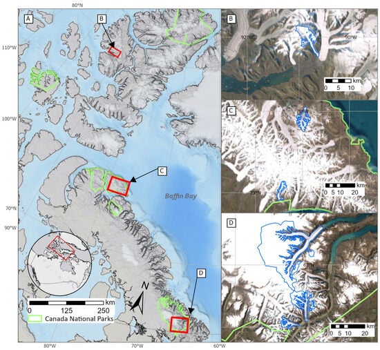
Figure 1. Study area overview showing three key glacier regions in the Canadian Arctic Archipelago (CAA). (A) Regional map highlighting the locations of the detailed study areas (red boxes) on Axel Heiberg Island, Bylot Island, and Baffin Island, with the boundaries of Canadian National Parks outlined in green. Panels (B–D) show high-resolution satellite imagery of glacierized regions: (B) White Glacier on Axel Heiberg Island; (C) glaciers on Bylot Island within Sirmilik National Park; and (D) glaciers in Auyuittuq National Park on southern Baffin Island. Glacier outlines (blue) are from the Global Land Ice Measurements from Space (GLIMS) database (version dated 7 June 2023). Background imagery is from World Imagery (Esri, Maxar, Earthstar Geographics, and the GIS User Community; ArcGIS pro 3.2.2 Living Atlas of the World, Esri, accessed April 2025).

2.1. Auyuittuq National Park (ANP)

ANP (Figure 1D), meaning “the land that never melts” in Inuktitut, encompasses the Penny Ice Cap (PIC), the largest ice mass in the Southern CAA. The park features deep fjords and glaciated valleys. This study examines Highway Glacier (93.97 km²) and Turner Glacier (28.77 km²), both of which are typical alpine valley glaciers flowing from the PIC. These glaciers are typical alpine valley glaciers bordered by peaks and nunataks. Akshayuk Pass, a well-known hiking corridor, attracts approximately 250 visitors annually and serves as an essential travel route between Pangnirtung and Qikiqtarjuaq for local residents.

In 2022, in collaboration with Parks Canada and the Ice Climate Environmental Laboratory (ICElab) at Queen’s University, glacier monitoring on Turner Glacier began, involving the installation of 10 stakes at elevations from 500 m to 1700 m. This network sought to measure mass balance and could serve as validation for remote sensing estimates of glacier changes in the region (see [21]).

Glaciological Fieldwork Report on Turner Glacier (2022–2023)). The area experiences a polar marine climate with long, cold winters and short, cool summers. Based on Sentinel-2 satellite data from 2013–2024, summer melt typically starts in late May and ends by early September. An automatic weather station (AWS) at Owl River (Lat: 66.880, Lon: −64.696) recorded an mean annual air temperature of −9.82 °C from 2012 to 2023, with extremes ranging from 16.66 °C to −41.59 °C, and frequent humidity levels above 70% owing to the proximity of Baffin Bay.

Coronation Glacier, the largest outlet glacier of the PIC, extends approximately 35 km to its terminus in Coronation Fjord, covering about 655.01 km² with elevations ranging from 8 to 2017 m a.s.l. Historical data indicate a retreat rate of 12 m per year from 1890 to 1988 [22]. Recent observations, however, show an accelerated retreat, with approximately 800 m lost between 1989 and 2016, averaging 30 m per year [23]. This rapid retreat has led to the formation of a new island at the glacier’s terminus, an unexpected detail reflecting significant glacial dynamics in response to climatic changes.

2.2. Sirmilik National Park (SNP)

SNP (Figure 1C), translating to “place of glaciers” in Inuktitut, is situated on Bylot Island adjacent to Lancaster Sound. The island is heavily glaciated, with a 4500 km² icefield dominating its landscape [24]. Valley glaciers like Fountain (33.96 km², 245–1753 m a.s.l.) and BylotD20s (69.42 km², 129–1433 m a.s.l.) flow outward from their accumulation zones onto the lowlands. Fountain Glacier is polythermal, with a warm core insulated by cold marginal ice, facilitating pressurized subglacial water storage and periodic proglacial icing regeneration [25]. BylotD20s, identified as a surge-type glacier by Dowdeswell et al. [24], undergoes periodic rapid advances followed by quiescence, a characteristic behavior of such glaciers in the Canadian Arctic.

The climate in SNP is governed by high-latitude seasonality and marine influences from Lancaster Sound. Winters are long and cold, with wind chill frequently intensifying exposure, whereas summers are brief and cool, restricting the duration of glacier melt. Snowfall is moderate, but persistent winds redistribute snow, modulating accumulation patterns [24]. The park’s proximity to Bylot Island and Lancaster Sound, and their effects on sea ice and ocean currents, shapes the local microclimate and influences the timing and extent of melt–refreeze cycles [24]. In 2023, in partnership with Parks Canada and ICElab at Queen’s University, glacier monitoring on Fountain Glacier was initiated, establishing a network of seven stakes spanning 500–1400 m a.s.l. was installed, together with an AWS at 1400 m (Lat: 73.055, Lon: −78.412).

2.3. Axel Heiberg Island (AHI)

White Glacier (Figure 1B), located on the southern margin of AHI (79.750°N, 91.117°W), serves as the long-term benchmark for this study. It has a continuous record of glaciological observations reported to the World Glacier Monitoring Service [26]. The mean annual temperature is approximately −20 °C. Precipitation ranges from 58 mm a⁻¹ at sea level to 370 mm a⁻¹ at higher elevations, as recorded at the Eureka weather station (~100 km northeast) [12]. Field-measured ELA from White Glacier provide the primary validation for the machine-learning-derived SLAs in this study.

3. Data

3.1. Optical Satellite Imagery

Approximately 9920 multispectral satellite images from three freely accessible datasets, Landsat 8/9 Surface Reflectance (SR), Sentinel-2 SR (Level-2A), and Sentinel-2 Top-of-Atmosphere (TOA, Level-1C), were utilized in this study (Table 2). Image acquisition spanned the decade from 2013 to 2024, focusing on the summer melt season (1 June to 30 September), and enabled detailed temporal analyses of snowline dynamics across the study area (Table 3). All imagery was accessed and processed in GEE, which supported scalable classification and snowline delineation workflows.

Table 2. Summary of optical satellite imagery (Landsat 8/9 SR, Sentinel-2 TOA, and Sentinel-2 SR) processed for the six study glaciers (2013–2024).

Glacier	Landsat 8/9 SR	Sentinel-2 TOA	Sentinel-2 SR	Total Scenes
ANP
Highway	260	553	435	1248
Turner	229	501	372	1102
Coronation	364	631	447	1442
SNP
Fountain	268	904	694	1866
BylotD20s	357	910	696	1963
AHI
White	748	882	669	2299
Total	2226	4381	3313	9920

Table 3. Characteristics of the satellite datasets used in this study. SR = Surface Reflectance; TOA = Top-of-Atmosphere; OLI = Operational Land Imager; MSI = MultiSpectral Instrument.

Satellite Dataset	Product Type	Revisit	Temporal Coverage	Spectral Range (μm)	Spatial Res. (m)
Landsat 8/9 (OLI)	SR (Level-2)	16 d (8 d L8 + L9)	2013– (L8); 2021– (L9)	0.43–2.29 (VNIR–SWIR)	30
Sentinel-2 A/B (MSI)	SR (Level-2A)	5 d (A + B)	2015– (S2A); 2017– (S2B)	0.44–2.20 (Vis–NIR–SWIR)	10/20/60 a
Sentinel-2 A/B (MSI)	TOA (Level-1C)	5 d (A + B)	2015– (S2A); 2017– (S2B)	0.44–2.20 (Vis–NIR–SWIR)	10/20/60 a

^a Sentinel-2 native ground sampling distances are 10 m (B2–B4, B8), 20 m (B5–B7, B11–B12), and 60 m (B1, B9, B10). Unless otherwise stated, analyses in this study use the 10 m visible and near-infrared bands (B2–B4, B8).

Each dataset possesses distinct spectral characteristics. Landsat 8/9 SR provides seven spectral bands spanning 0.43–2.29 µm at 30 m spatial resolution. Sentinel-2 (A and B) delivers 12 bands across 0.44–2.20 µm, with 10 m resolution in the visible and near-infrared (B2–B4, B8), 20 m in the red-edge and shortwave-infrared (B5–B7, B11–B12), and 60 m in atmospheric bands (B1, B9, B10) (Table 3). Thus, the 0.44–2.20 µm range samples the visible (0.4–0.7 µm), near-infrared (0.7–1.3 µm), and shortwave-infrared (1.5–2.5 µm) portions of the electromagnetic spectrum. The combination of Sentinel-2A and -2B yields an effective revisit of 5 days, enhancing temporal coverage for seasonal glacier-surface assessments. In this study, unless stated otherwise, we use the 10 m visible and near-infrared bands (B2–B4, B8) for analysis.

3.2. Glacier Outline

Glacier outlines for each study site were obtained from the GLIMS database, version dated 7 June 2023 [4,27]. Glacier boundaries were accessed via the GEE ee.FeatureCollection (“GLIMS/20230607”), using the designated Analysis IDs for each glacier. These outlines served two primary functions: (1) clipping satellite imagery to each glacier’s extent during data querying and (2) defining the spatial domain for calculating SCA and extracting SLA.

3.3. Digital Elevation Model

Topographic data used for SLA determination were sourced from ArcticDEM Version 3 (2 m mosaic), released in September 2018 and distributed by the Polar Geospatial Center, University of Minnesota. This dataset is derived from stereophotogrammetric processing of imagery acquired between 2007 and 2017 [28]. The reported vertical accuracy is ~4 m (RMSE), although actual errors vary with terrain complexity, slope, and image acquisition geometry [28,29]. These uncertainties were considered when interpreting SLA and related metrics.

3.4. Meteorological Records

Meteorological time series were sourced from the Historical Climate Data archive maintained by Environment and Climate Change Canada (ECCC) (https://climate.weather.gc.ca/, accessed on 5 August 2025). The primary parameters utilized include daily mean air temperature ($T_d$, °C), daily maximum air temperature ($T_{max}$, °C), and daily total precipitation ($P_d$, mm). These data were retrieved from three stations—Pangnirtung (ANP), Pond Inlet (SNP), and Eureka (AHI)—to calculate derived metrics including seasonal mean temperatures (JJA and DJF) and annual Positive Degree Days (PDD), which serve as proxies for melt-season intensity. To ensure data quality, years containing more than 30 missing daily observations were excluded from the trend analysis.

4. Method

The methodological pipeline was implemented in Python 3.11.11, following the framework adapted from Aberle et al. [20], with modifications tailored specifically for this study. The principal changes were: (i) classification restricted to glacier polygons and defined as a binary separation of snow versus bare ice (rather than snow versus non-snow) and (ii) estimation of SLA from the SCR using elevation binning.

4.1. Data Acquisition

Multi-spectral imagery from the Sentinel-2 SR, Sentinel-2 TOA, and Landsat 8/9 SR archives was accessed via the GEE cloud-computing platform. To capture the state of the glacier surface during the peak ablation season, scenes were filtered for acquisition dates between 1 June and 30 September for the period 2013–2024. Selection was further constrained to scenes with <20% cloud cover and >60% spatial overlap with the area of interest (AOI).

All imagery was reprojected to the local UTM zone and processed at the native spatial resolutions of the respective sensors (10 m for Sentinel-2; 30 m for Landsat). Rather than resampling to a common grid, machine learning classifiers were applied independently to each sensor’s archive. This sensor-specific approach preserves the high-frequency spatial detail inherent in the Sentinel-2 data, optimizing the precision of the SCR and subsequent snowline extraction. Topographic context for snowline delineation was provided by the ArcticDEM (Version 3.0) mosaic, which was co-registered and clipped to the AOI.

4.2. Data Preprocessing

Image preprocessing involved the application of sensor-specific scale factors and cloud masking. Subsequently, the imagery was rescaled and normalized. To support accurate classification of snow and ice surfaces, the Normalized Difference Snow Index (NDSI) was computed for each image using the standard formulation [30]:

$$\mathrm{NDSI}={\displaystyle \frac{\mathrm{Green}-\mathrm{SWIR}}{\mathrm{Green}+\mathrm{SWIR}}}$$

(1)

where Green refers to reflectance in the green band (Landsat 8/9: B3, 0.53–0.59 µm; Sentinel-2: B3, 0.54–0.58 µm) and SWIR denotes reflectance in the shortwave-infrared band. For Landsat8/9, SWIR was taken from B6 (1.57–1.65 µm; 30 m). For Sentinel-2, SWIR was taken from B11 (1.56–1.66 µm; 20 m). All indices were computed at the sensors’ native spatial resolution.

4.3. Image Classification

Supervised machine learning techniques were applied to the preprocessed multispectral imagery, adapting the workflow and pre-trained classifier of Aberle et al. [20] with study-specific modifications. To accommodate sensor-dependent band configurations and radiometry, separate classifiers were maintained for each archive. For Landsat surface-reflectance imagery, a nearest-neighbor (NN) classifier was found to be optimal, whereas a support vector machine (SVM) delivered superior performance for Sentinel-2 datasets (both surface reflectance and top-of-atmosphere products).

The scheme mapped five land-cover classes: snow, shadowed snow, bare ice, rock, and water. Classifications were restricted to glacier polygons and exported as GeoTIFF files for subsequent analyses. For quality control, each classified raster was paired with a natural-color composite for visual validation.

4.4. Snowline Delineation

Snowline delineation was performed using two complementary approaches: (i) Snow Elevation Histogram Analysis (SEHA; [20]) and (ii) an elevation-bin method. A comparison for Highway Glacier is shown in Figure 2, illustrating the classified snowline location, associated elevation bins, and the SCR metrics.

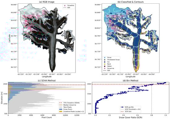
Figure 2. Snowline delineation comparison for Highway Glacier (21 August 2020) using Sentinel-2 Surface Reflectance imagery. (a) RGB composite with the delineated snowline and area of interest (AOI) extent. (b) Supervised classification map showing snow, shadowed snow, bare ice, rock, and water with elevation contours. (c) SEHA method: pixel-elevation histogram of snow-covered classes used to derive the median snowline altitude (${\mathrm{SLA}}_{\mathrm{SEHA}}$). (d) Elevation-bin method: SCR per 10 m bin from ArcticDEM v3, with ${\mathrm{SLA}}_{\mathrm{bin}}$ defined at the 0.8 threshold.

4.4.1. SEHA

SEHA delineates the snowline from the hypsometric distribution of snow-covered pixels [20]. To reduce noise from small patches and high-contrast artefacts (e.g., crevasses, bedrock protrusions), the classified image was refined by edge detection and morphological hole-filling within the snow-covered area, under the assumption that elevation exerts the dominant control near the end of the melt season. Two 10 m elevation histograms were constructed: one for all glacier pixels and one for snow-covered pixels (snow + shadowed snow). The AAR in elevation bin k was computed as

$${\mathrm{AAR}}_k={\displaystyle \frac{N_{\mathrm{snow},k}}{N_{\mathrm{glacier},k}}}$$

(2)

where $N_{\mathrm{snow},k}$ and $N_{\mathrm{glacier},k}$ are the numbers of snow-covered and total glacier pixels, respectively. For standardization, bins with ≥75% snow cover were set to 100% to enforce continuity in the mapped snow mantle, and a binary mask (snow vs. ice) was generated. Snowline contours were then extracted at snow–ice boundaries; elevations were sampled from the DEM along the contour vertices, and the median of these elevations defined ${\mathrm{SLA}}_{\mathrm{SEHA}}$.

4.4.2. Elevation-BinSnowline Delineation

Following Rastner et al. [15] and validated for White Glacier [18], the elevation-bin method estimates the snowline from the SCR. The glacier surface was partitioned into 10 m elevation bins spanning the full hypsometric range. In bin k,

$${\mathrm{SCR}}_k={\displaystyle \frac{N_{\mathrm{snow},k}}{N_{\mathrm{snow},k}+N_{\mathrm{ice},k}}}$$

(3)

i.e., the fraction of snow-covered pixels relative to the snow + ice surface within the glacier polygon, which reduces sensitivity to outline uncertainties. The snowline altitude, ${\mathrm{SLA}}_{\mathrm{bin}}$, was defined as the lowest elevation in the first run of ≥3 consecutive bins with $\mathrm{SCR}\ge 0.8$; if no such run existed, the lowest bin with $\mathrm{SCR}\ge 0.8$ was selected.

4.4.3. Snowline Metrics and Analysis

Each classified maps and the DEM were used to derive four glaciologically relevant metrics: SCA, AAR, SCR, and SLA.

• SCA. Total mapped snow area (including shadowed snow), computed as

  $$\mathrm{SCA}=N_{\mathrm{snow}}{A}_{\mathrm{px}},$$

  (4)

  where $N_{\mathrm{snow}}$ is the number of snow pixels and $A_{\mathrm{px}}$ is pixel area; reported in km². This represents the seasonal/perennial snow extent at the acquisition time.
• AAR. Fraction of the glacier that is snow covered:

  $$\mathrm{AAR}={\displaystyle \frac{\mathrm{SCA}}{A_{\mathrm{glacier}}}},$$

  (5)
  Although widely used, AAR is sensitive to outline uncertainties, particularly for debris-covered or small glaciers.
• SCR. Proportion of snow-covered pixels (snow + shadowed snow) relative to the combined snow + ice surface within the glacier polygon:

  $$\mathrm{SCR}={\displaystyle \frac{N_{\mathrm{snow}}}{N_{\mathrm{snow}}+N_{\mathrm{ice}}}},$$

  (6)
  SCR reduces sensitivity to glacier-boundary error and is useful for characterizing vertical snow distribution and estimating snowlines.
• SLA The transient boundary between snow-covered and bare-ice surfaces. Two estimates are used:

  1.

  ${\mathrm{SLA}}_{\mathrm{SEHA}}$: Median elevation of snow–ice boundary contours derived with SEHA after setting elevation bins with ≥75% snow cover to 100% and generating a binary (snow/ice) mask.

  2.

  ${\mathrm{SLA}}_{\mathrm{bin}}$: From the elevation-bin method, defined as the lowest elevation in the first run of ≥3 consecutive bins with $\mathrm{SCR}\ge \tau$ (with $\tau =0.8$). If no such run exists, the lowest bin with $\mathrm{SCR}\ge \tau$ is used.

The annual SLA is intended to represent end of ablation season conditions, when seasonal snow extent is close to its minimum and the snowline is near its highest elevation. For each year, all available cloud free late summer optical scenes were evaluated and selected the scene representing minimum SCR. This single-scene approach was chosen because multi-temporal compositing can ‘smear’ the transient snowline signal, averaging different stages of retreat and resulting in an SLA that lacks physical consistency with the true seasonal maximum [14,15]. In years where only one suitable late summer cloud free scene was available, that scene was used as the best available approximation of end of season conditions.

4.5. Uncertainty Assessment

Estimates of the transient SLA are subject to uncertainties arising from (i) image classification, (ii) sensor spatial resolution, (iii) the delineation methodology, and (iv) DEM vertical accuracy.

4.5.1. Classification Uncertainty

Classification uncertainty stems from the quality and representativeness of training labels and from algorithm performance (e.g., NN, SVM). In this study, classifiers were initialized from the manually labelled US West Coast benchmark dataset of Aberle et al. [20], which was validated by glaciological experts. Accuracy was assessed using confusion matrices across snow, ice and land classes; per-class user’s/producer’s accuracies and overall accuracy were examined. To further ensure reliability, each classified scene was visually checked against natural-color composites by the author, informed by field experience in the study area.

Despite these measures, residual classification errors propagate into glaciological metrics, though their impact remains unquantified in this analysis due to the complexity of error propagation across scales.

4.5.2. Spatial Resolution of Input Imagery

Sentinel-2 imagery (10 m resolution) and Landsat 8/9 imagery (30 m resolution) were utilized, introducing inherent resolution-dependent uncertainty in the estimation of SCA, AAR, and SCR. However, because the SLA is derived from elevation-binning (SCR-based) rather than pixel-scale horizontal delineation, the difference in spatial resolution does not introduce a significant vertical bias. The SCR is calculated as an area-weighted fraction within discrete 10 m elevation bins; therefore, while coarser pixels may increase horizontal uncertainty at the snow-ice boundary, the vertical signal remains consistent across platforms as long as the glacier width significantly exceeds the pixel size. By treating the sensors as independent inputs within the ML pipeline, potential resolution-dependent biases, which often arise from forced data merging or resampling, were avoided. Consequently, SCR calculations for each scene were derived using the optimal spatial and spectral configurations specific to the individual sensor. It is recognized that coarser-resolution imagery may obscure small-scale snowline features, particularly in regions of complex topography. While this uncertainty was not explicitly quantified in the current study, it is acknowledged as a contributing factor to the error budget. Sentinel-2 imagery was prioritized where available to enhance spatial precision and minimize resolution-related artifacts in the final datasets.

4.5.3. Snowline Delineation and Elevation Data

All SLA estimates were derived using ArcticDEM v3 mosaic data (2007–2017), which reports a vertical accuracy of ±4 m [29]. However, uncertainties may increase locally due to terrain slope, surface roughness, acquisition geometry, and temporal mismatches between the DEM and satellite imagery (2013–2024). These temporal mismatches may lead to unaccounted glacier surface changes (e.g., thinning, accumulation), which are not incorporated here due to their relatively minor expected influence and the absence of time-resolved elevation data for individual glaciers.

Method-specific contributions arise from the discretisation of the 10 m elevation bins used in both approaches:

• SEHA: SLA is the median elevation of mapped snow–ice contours derived after histogram-based adjustment; the 10 m binning implies a vertical quantization uncertainty of $\pm 5$ m.
• elevation-bin method: SLA is the lowest elevation in the first run of ≥3 bins with $\mathrm{SCR}\ge 0.8$; the same binning implies ±5 m.

4.5.4. Combined Uncertainty in Snowline Altitude

To estimate the total vertical uncertainty in SLA, a root-sum-square (RSS) method is used, combining the vertical uncertainty of the ArcticDEM and the method-specific binning uncertainty:

$${\sigma }_{\mathrm{SLA}}=\sqrt{{\sigma }_{\mathrm{DEM}}^2+{\sigma }_{\mathrm{method}}^2}$$

(7)

where ${\sigma }_{\mathrm{DEM}}=\pm 4$ m and ${\sigma }_{\mathrm{method}}=\pm 5$ m.

These values represent conservative uncertainty bounds under the assumption that DEM and methodological uncertainties are independent. Other potential contributors, including classification error, local slope variability, and temporal DEM-image mismatches, are acknowledged but not explicitly quantified due to data limitations.

4.6. Meteorological Data Preprocessing

Seasonal and Annual Metrics

Meteorological diagnostics were derived for each station and year y using daily mean air temperature $T_d$ (°C) and daily total precipitation $P_d$ (mm). The following indices were computed:

1.

JJA mean temperature (June–August): mean daily air temperature over June, July, and August. Seasonal means were retained only if fewer than 30 days were missing.

2.

DJF mean temperature (December–February): mean daily air temperature over December of year $y-1$ and January–February of year y; results are attributed to season year y. Seasons with ≥30 missing days were excluded.

3.

Annual precipitation (mm): sum of daily total precipitation for calendar year y, retained only if fewer than 30 days were missing.

4.

Positive Degree Days (PDD; °C d): sum of daily mean air temperatures above 0 °C for calendar year y:

$${\mathrm{PDD}}_y=\sum _{d\in \mathrm{Year}\left(y\right)}max\left(0,T_d\right),$$

(8)

retained only if fewer than 30 days were missing.

All time series were reindexed to a common temporal range (1960–2024), with missing values retained where data were unavailable.

4.7. Trend Estimation

Trends in JJA and DJF mean temperatures and PDD (precipitation excluded) were estimated using ordinary least squares (OLS) applied to each contiguous segment of ≥10 years with complete data. For a segment comprising years $\{x_1,\dots ,x_n\}$ and values $\{y_1,\dots ,y_n\}$, a linear model $y=a+bx$ was fitted. Slopes were scaled to units of per decade (e.g., °C/decade) and reported with two-sided p-values from a t-test on the slope coefficient. Segments shorter than 10 years were excluded from trend analysis.

5. Results

5.1. Annual SCA (2013–2024)

Analysis of annual SCA trends (June–September) reveals consistent seasonal oscillatory patterns in snow cover from 2013 to 2024. Figure 3 illustrates these patterns across six glaciers, capturing the progression of the seasonal ablation cycle: snow cover begins to decline in June, reaches a minimum extent in July or August, and partially recovers by September. The integration of Sentinel-2 data post-2016 enhances temporal resolution compared to Landsat alone, offering a more detailed view of the ablation season’s evolution.

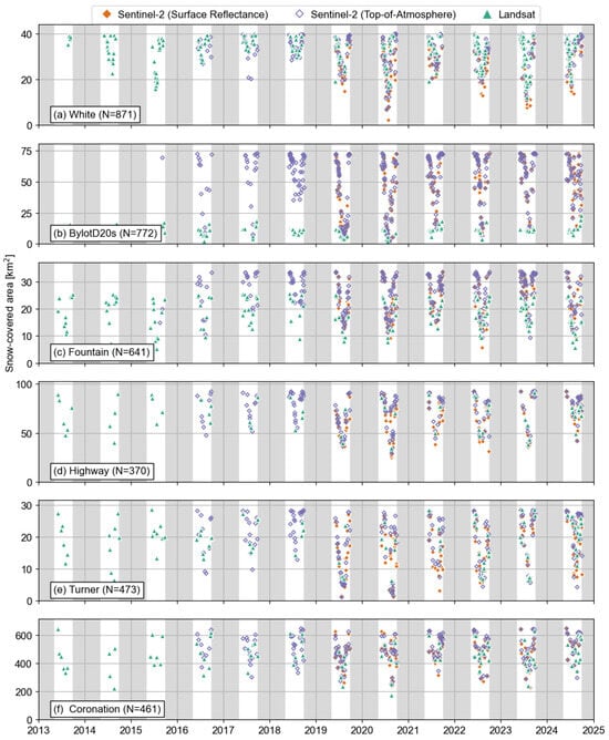
Figure 3. Annual Snow-Covered Area (SCA) (2013–2024) for six Arctic glaciers. Time series of snow-covered area (SCA) for six Canadian Arctic glaciers from 2013 to 2024: (a) White, (b) BylotD20s, (c) Fountain, (d) Highway, (e) Turner, and (f) Coronation. Data sources include Sentinel-2 Surface Reflectance (orange diamonds), Sentinel-2 Top-of-Atmosphere (purple hollow diamonds), and Landsat (green triangles). Grey vertical bands denote winter periods (October–May). N indicates the number of observations per glacier.

5.1.1. Regional SCA Trends: Interannual Variability

From White Glacier in the High Arctic to Coronation Glacier in the southeast, interannual variability in SCA is evident. White Glacier (Figure 3a) on Axel Heiberg Island experienced moderate fluctuations prior to 2020, followed by near-complete snowmelt events in 2020 ($\mathrm{SCA}\approx 0{\mathrm{km}}^2$). Notably, post-2020 observations reveal a partial recovery in snow-covered area, though maximum SCA remains consistently lower than in the pre-2020 period. Further south, BylotD20s (Figure 3b) in SNP regularly approaches zero SCA in late summer, reflecting its high sensitivity to atmospheric warming during peak ablation. Fountain Glacier (Figure 3c) maintains relatively stable minimal snow cover (<10 ${\mathrm{km}}^2$) during peak ablation.

5.1.2. Data Consistency and Image Availability

The SCA estimates derived from Landsat and Sentinel-2 imagery are generally consistent, though differences in spatial resolution and revisit frequency introduce some variability. Prior to 2016, the reliance on Landsat, with its 16-day revisit cycle, limited the temporal resolution of ablation season monitoring. A clear example is 2013, when White Glacier was only imaged once, in mid-to-late September, near the end of the melt season. While this single acquisition provided an important initial data point for long-term SCA and SLA analysis, it likely overestimated residual snow cover and may have biased early snowline altitude estimates. The 2015 launch of Sentinel-2 dramatically improved image availability, enabling higher temporal resolution and finer spatial detail. This enhancement was especially critical for detecting snowline dynamics and residual snow during the narrow late-summer ablation window. The increased revisit frequency also mitigated data loss due to cloud cover and allowed for more reliable multi-sensor fusion.

Regional disparities in cloudiness further affected image availability and data reliability. White Glacier, located in the relatively dry High Arctic, had the highest number of usable observations ($N=871$), enabling robust trend detection. In contrast, Coronation Glacier—subject to persistent maritime cloud cover—had the fewest observations ($N=461$). Among the mid-latitude glaciers, data density declined with decreasing latitude: Fountain ($N=641$), Turner ($N=473$), and Highway ($N=370$), with Highway experiencing the lowest data availability, likely reflecting increased cloudiness at lower elevations and more humid conditions.

5.1.3. Intra-Annual Variability of Weekly Median Glacier Metrics

In ANP, both Highway and Turner Glaciers (Figure 3d,e) maintained relatively consistent peak ablation seasonal SCA prior to 2019. However, a pronounced decline was observed in subsequent years. Turner Glacier in particular experienced a significant reduction, reaching zero SCA in several post-2019 years, indicative of near-complete snowline retreat and intensified melt conditions. Similarly, Highway Glacier recorded multiple years of markedly reduced SCA, underscoring a significant shift in surface mass balance behavior. Coronation Glacier (Figure 3f), the southernmost site, shows greater fluctuation but recorded its lowest value (<200 ${\mathrm{km}}^2$) in 2020. The year of 2020 thus emerged as a widespread extreme melt year, particularly affecting glaciers in the central and southern CAA. Residual snow cover in Coronation and Highway glaciers during these years suggests regional variability in melt intensity and snow persistence.

5.1.4. Seasonal SCA Trends and Transient AAR Dynamics

Across all study regions, the seasonal evolution of SCA follows a characteristic cycle: high values in June, a pronounced minimum in August, and partial recovery in September. This pattern reflects the seasonal ablation–accumulation balance, with the lowest SCA values typically coinciding with peak summer melt. Glacier-to-glacier differences in the magnitude of SCA decline are influenced by factors such as latitudinal position, maximum glacier elevation ($Z_{\max }$), and local climate conditions.

Among smaller glaciers (<40 km²), White Glacier (Figure 4a) in the High Arctic displays a relatively narrow SCA range, consistent with the colder regional climate and reduced ablation intensity. In contrast, lower-latitude glaciers such as Fountain and Turner (Figure 4i,q), located in ANP and SNP, respectively, exhibit more pronounced seasonal declines in SCA during peak ablation, indicative of stronger summer melt. Despite their southern or mid-latitude positions, Highway and Coronation glaciers (Figure 4m,u) exceed 100 km² in area and have $Z_{\max }$ values over 2000 m, enabling greater snowpack preservation and dampening seasonal SCA variability.

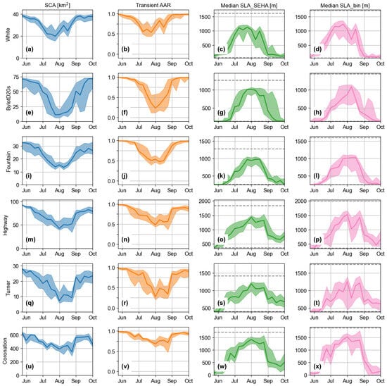
Figure 4. Seasonal evolution of glacier surface conditions for six Arctic glaciers—White, BylotD20s, Fountain, Highway, Turner, and Coronation—arranged from north to south, covering the ablation season from June to September (2013–2024). Each row corresponds to a glacier, and columns display: (a,e,i,m,q,u) snow-covered area (SCA) in blue, (b,f,j,n,r,v) transient accumulation-area ratio (AAR) in orange, (c,g,k,o,s,w) median snowline altitude (SLA) estimated using the SEHA method in green, and (d,h,l,p,t,x) median SLA estimated using the binning method in pink. The solid lines represent the weekly median values across all years (2013–2024), while the shaded areas indicate the interquartile range (Q1–Q3), reflecting seasonal variability. Grey dashed lines in the SLA panels mark the minimum and maximum SLA values for reference.

Transient AARs, calculated by normalizing SCA to total glacier area, reveal comparable seasonal snow depletion patterns across glaciers of varying sizes. Interestingly, smaller glaciers such as White and Fountain (Figure 4b,j) often show AARs similar to larger glaciers like Highway (Figure 4n), suggesting that relative snow loss is not necessarily dependent on glacier size. Glaciers with lower $Z_{\max }$ values—such as BylotD20s and Turner (Figure 4f,q)—frequently fall below an AAR of 0.5 in mid-summer, reflecting extensive ablation. Their maximum elevations (BylotD20s: 1433.26 m; Turner: 1684.84 m) are lower than those of most other glaciers in this study, which typically exceed 1700 m. In contrast, larger glaciers with extensive high-elevation accumulation zones, including Coronation and Highway, tend to maintain higher AARs throughout the melt season despite their more southerly locations. For example, during the extreme 2020 melt season, Coronation and Highway glaciers retained transient AARs of 0.50 and 0.48, respectively, while the lower-elevation Turner and BylotD20s glaciers reached AARs of 0.00.

Shaded regions in the SCA and AAR time series denote the interquartile range (Q1–Q3), capturing intra-seasonal variability linked to local topography, surface albedo, and transient weather conditions. For instance, BylotD20s and Turner glaciers are situated in steep terrain with complex shading and frequent cloud cover. These features amplify variability in seasonal melt signals and underscore the role of topographic complexity in modulating snow cover dynamics.

5.1.5. Median SLA Trends

SLA was estimated throughout the melt season using two approaches: SLA_SEHA (green) and SLA_bin (pink), as shown in Figure 4. Despite methodological differences, both approaches exhibit consistent seasonal behavior, progressive snowline ascent from June to August, followed by a descent during September. Across most glaciers, peak SLA values occur between approximately 1000 and 1500 m during maximum melt, decreasing to 700–1000 m by late September.

While the two methods agree in general trend, systematic differences are observed. SLA_bin tends to yield higher snowline estimates than SLA_SEHA. Additionally, SLA_bin displays broader interquartile ranges, indicating greater sensitivity to elevation-dependent heterogeneity in snow distribution. A more detailed assessment of SLA behavior during peak ablation is presented in the following section.

5.2. Annual Peak SLA from SEHA and Elevation-Bin Methods, and Relation to Summer Warmth (PDD), 2013–2024

Annual maximum SLA, derived with the SEHA (SLA_SEHA) and elevation-binning (SLA_bin), exhibited pronounced interannual variability across all six glaciers (Figure 5). The right axes plot PDD (°C·day) from the nearest long-term meteorological stations (Eureka for White; Pond Inlet for Bylot D20s and Fountain; Pangnirtung for Highway, Turner, Coronation). Notably, Highway Glacier attained the highest SLA in 2020: ${\mathrm{SLA}}_{\mathrm{SEHA}}$ = 1835 ± 6 m and ${\mathrm{SLA}}_{\mathrm{bin}}$ = 1995 ± 6 m, exceeding all other observations in the record.

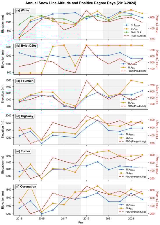
Figure 5. Annual peak snowline altitude (SLA) during the ablation season (1 June–30 September) for 2013–2024 across six glaciers in the Canadian Arctic, derived using two approaches: (i) Snow Elevation Histogram Analysis (${\mathrm{SLA}}_{\mathrm{SEHA}}$) and (ii) an elevation-bin method (${\mathrm{SLA}}_{\mathrm{bin}}$; 10 m bins; SCR threshold $\tau =0.8$). Panel (a) additionally shows field-based SLA observations for White Glacier. Glaciers: (a) White Glacier (Axel Heiberg Island), (b) BylotD20s Glacier, (c) Fountain Glacier (Sirmilik National Park, Bylot Island), (d) Highway Glacier, (e) Turner Glacier, and (f) Coronation Glacier (Auyuittuq National Park, Baffin Island).

5.2.1. Sensitivity to Summer Warmth

${\mathrm{SLA}}_{\mathrm{bin}}$ was positively correlated with PDD at most sites, with glacier-specific sensitivities (slope of ${\mathrm{SLA}}_{\mathrm{bin}}$ vs. PDD in m °C⁻¹ d): White ≈ 2.56 m °C⁻¹ d ($r=0.76$, $p=0.0039$); Highway ≈ 0.67 m °C⁻¹ d ($r=0.60$, $p=0.039$); Turner ≈ 0.83 m °C⁻¹ d ($r=0.58$, $p=0.049$). Weaker correlations were observed at Fountain ($r=0.39$, $p=0.21$), BylotD20s ($r=0.35$, $p=0.27$), and Coronation ($r=0.18$, $p=0.57$). ${\mathrm{SLA}}_{\mathrm{SEHA}}$ showed similar but generally weaker correlations with PDD. Years with high PDD typically coincide with higher SLAs (e.g., 2019–2021 at several sites), whereas relatively cool summers (e.g., 2015 at multiple sites) correspond to lower SLAs, consistent with the visual patterns in Figure 5.

5.2.2. Spatial and Temporal Patterns of SLA

Peak SLA values generally occurred in warm summers, though the year of maximum SLA varied by site (SLA_bin maxima: White, 2023: 1705 m; Fountain, 2023: 1595 m; Highway, 2020: 1995 m; Turner, 2021: 1745 m; Coronation, 2014: 1885 m; BylotD20s: multiple years, 2017–2024, range: 1435–1445 m). Minimum SLAs were typically recorded during cooler summers, notably 2015 across multiple Baffin Island glaciers. Across the study region, glaciers in ANP exhibited consistently higher SLA values compared to those in SNP and the Eureka region, consistent with warmer summer conditions. All regions displayed a positive SLA–PDD relationship, strongest at White Glacier.

5.2.3. Comparison Between SLA Methods (${\mathrm{SLA}}_{\mathrm{bin}}$ vs. ${\mathrm{SLA}}_{\mathrm{SEHA}}$)

At five of the six sites (BylotD20s, Fountain, Highway, Turner, Coronation), SLA_bin was systematically higher than SLA_SEHA, with a median offset of 164 m (range of site medians: 89–203 m). White Glacier was an exception, exhibiting near-zero median offset (+10 m) but a larger interquartile range (−249 to +146 m), driven primarily by a low 2013 SLA_bin value. These differences reflect the greater selectivity of the elevation-binning method under high snow-covered ratio thresholds and the tendency for histogram peaks to fall below the highest clean snowline pixels (Figure 5). The time series also revealed abrupt SLA increases. In 2016, BylotD20s SLA_bin rose from approximately 850 m to nearly 1400 m. Coronation SLA_SEHA exceeded 1500 m from 2018 onward, and White SLA_SEHA rose above 1500 m in 2019 and remained at or above that level thereafter. These episodes likely reflect anomalously high ablation, low accumulation, or both, with a possible contribution from methodological sensitivity.

5.2.4. Validation Against Field-Derived ELA (White Glacier)

Over the full period with available field ELA data (2013–2023), ${\mathrm{SLA}}_{\mathrm{bin}}$ tracks ELA well ($r=0.88$, $p<0.001$; $\mathrm{RMSE}=298 \mathrm{m}$; mean bias $\Delta \mathrm{ELA}={\mathrm{SLA}}_{\mathrm{bin}}-\mathrm{ELA}=-60 \mathrm{m}$; 95% CI $[-265 \mathrm{m},+145 \mathrm{m}]$; $n=11$). For the recent, denser period (2019–2023), ${\mathrm{SLA}}_{\mathrm{bin}}$ retains a strong correlation ($r=0.87$, $p=0.054$) with $\mathrm{RMSE}=214 \mathrm{m}$ and a mean positive bias of $+170 \mathrm{m}$ (95% CI $[-11 \mathrm{m},+350 \mathrm{m}]$; $n=5$). ${\mathrm{SLA}}_{\mathrm{SEHA}}$ also correlates with ELA over 2019–2023 ($r=0.55$, $p=0.34$; $\mathrm{RMSE}=165 \mathrm{m}$; mean bias $+100 \mathrm{m}$, 95% CI $[-82 \mathrm{m},+282 \mathrm{m}]$).

A complementary analysis over the full comparison period (Figure 5a) yielded consistent results. The SEHA method exhibited a mean positive bias of +164.9 m and RMSE of 339.2 m, whereas the elevation-bin method showed a smaller mean bias of +53.4 m and RMSE of 177.0 m. Elevation-bin SLA was strongly correlated with field ELA ($r=0.82$, $p=0.0039$), while SEHA exhibited a weak negative correlation ($r=-0.28$). Paired t-tests indicated no significant difference from field-derived ELA at the 95% confidence level (SEHA: $t=1.67$, $p=0.13$; elevation-bin method: $t=-0.95$, $p=0.37$).

These results indicate that both methods capture interannual ELA variability at White Glacier, with the elevation-bin method demonstrating stronger correlation, lower RMSE, and reduced bias. Residual differences likely result from image acquisition timing and mixed-pixel effects near the end-of-ablation period.

In summary, the results demonstrate that (i) the elevation-bin method consistently yields higher SLA estimates than histogram-based values at most sites; (ii) SLA increases with summer warmth, though sensitivity varies between glaciers; and (iii) on White Glacier, both satellite-derived SLA metrics reproduce interannual ELA variability, with method-specific biases likely attributable to image timing and mixed-surface conditions.

5.3. Regional Climatic Trends in the CAA: 1960–2024

Here, we analyze JJA and DJF mean air temperature, PDD, and annual precipitation at Pond Inlet, Pangnirtung, and Eureka (Figure 6). Trends were estimated by ordinary least squares over the periods displayed in each panel.

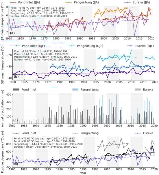
Figure 6. Annual climate indicators at Pond Inlet, Pangnirtung, and Eureka, 1960–2024: (a) JJA (June–August) mean temperature, (b) DJF (December–February) mean temperature, (c) annual precipitation, and (d) PDD (positive degree days). Dashed lines denote ordinary least squares linear trends over the periods stated on each panel; slopes (per decade) and p-values are annotated. Grey shading indicates decades.

5.3.1. Summer Temperature (JJA)

Mean summer temperature increased at all stations, with the steepest rate at Pangnirtung during its late 1990s–2010 interval. Pond Inlet (1999–2020) warmed by +0.59 °C decade⁻¹ ($p=0.033$), equivalent to ≈+1.88 °C across the fitted period. Pangnirtung (1996–2010) warmed by +0.95 °C decade⁻¹ ($p=0.0067$), or ≈+2.16 °C. Eureka (1960–2019) warmed by +0.35 °C decade⁻¹ (p < 0.001), totaling ≈+2.01 °C over six decades. These results indicate coherent summertime warming from the High Arctic (Eureka) to the more southerly setting (Pangnirtung); the larger Pangnirtung rate reflects its shorter, recent window capturing late 20th–early 21st century warming.

5.3.2. Winter Temperature (DJF)

Long records show significant winter warming, whereas shorter/noisier series are positive but not significant. Eureka (1960–2020) warmed by +0.41 °C decade⁻¹ (p = 0.0034). Trends at Pond Inlet (1998–2020; +0.64 °C decade⁻¹, p = 0.29) and Pangnirtung (1996–2010; +1.69 °C decade⁻¹, p = 0.22) are not statistically significant. Winter exhibits high interannual variability, but the six-decade Eureka record demonstrates statistically significant multi-decadal winter warming typical of the High Arctic.

5.3.3. Positive Degree Days (PDD)

PDD increases mirror the temperature trends, with significance governed by record length. Eureka (1960–2020) increased by +30.5 °C·day decade⁻¹ ($p\approx 9\times {10}^{-6}$). Increases at Pond Inlet (1999–2020; +39.9 °C·day decade⁻¹, $p=0.16$) and Pangnirtung (1996–2009; +64.0 °C·day decade⁻¹, $p=0.33$) are not statistically significant. Thermal forcing for melt has strengthened, clearly so at Eureka; the shorter Pond Inlet and Pangnirtung series show consistent but less certain positive tendencies.

5.3.4. Annual Precipitation

Interannual variability is large and station behavior is not uniform, and no regional, coherent multi-decadal signal is evident.

The three-station composite shows clear summer warming at all sites and significant winter warming where long records exist (Eureka). PDD increases track these temperature trends, implying greater melt potential in recent decades. Precipitation changes are spatially heterogeneous and comparatively muted.

6. Discussion

6.1. Regional Variability in Snowline Dynamics and Glacier Response

Seasonal SCA dynamics across the six study glaciers (Figure 3) exhibit the typical pattern of extensive early-summer snow cover, minima in mid-summer, and partial recovery by late summer. However, the amplitude of this seasonal cycle varies substantially among regions. White Glacier, located at high latitude and elevation, displays the narrowest seasonal range in SCA. In contrast, mid- to low-latitude glaciers with lower accumulation zones, BylotD20s and Turner, frequently reach near-total depletion $\mathrm{SCA}\approx 0{\mathrm{km}}^2$ during warm years. This spatial gradient reflects the underlying climate warming trend across the CAA and underscores the influence of glacier hypsometry on ablation sensitivity [31,32].

When normalized by glacier area, SCA trends indicate that glacier size is not the dominant control on summer snow retention (Figure 4). Glaciers of contrasting sizes, such as White and Fountain (small) and Highway and Coronation (large) show similar area-adjusted snow depletion trajectories. Instead, two primary factors govern summer snow retention: (i) the extent of high-altitude accumulation terrain and (ii) exposure to maritime versus continental air masses. This synoptic divide is a well-documented driver of mass-balance variability in the CAA; while White Glacier sits in a “polar desert” regime characterized by continental aridity [12], the southern glaciers on the Penny Ice Cap are exposed to moisture-laden maritime air masses from Baffin Bay [2]. These maritime influences bring increased humidity and cloud cover, which can enhance ablation via sensible heat flux. Despite their southerly latitudes, Coronation and Highway glaciers maintain late-season snow cover due to maximum elevations $Z_{max}$ > 2000 m, which provide a cold “headroom” for the migrating ELA. Conversely, Turner ($Z_{max}$ = 1685 m) and BylotD20s ($Z_{max}$ = 1433 m) lose their accumulation zones rapidly when the SLA surpasses approximately 1400 m. These findings suggest that glaciers with limited high-elevation terrain are particularly susceptible to high melt seasons, with hypsometry emerging as a key determinant of mass-balance resilience [33].

Cloud cover further modulates both melt processes and observational coverage. In the southern CAA, for example, persistent cloudiness over Coronation Glacier reduced the number of usable optical satellite scenes (N = 461), reflecting the influence of warm, moist air masses that enhance melt via sensible heat flux. Conway and Cullen [34] documented extended melt durations under overcast conditions on Brewster Glacier, New Zealand, a phenomenon potentially exacerbated in the absence of sufficient accumulation. Similarly, ref. [35] reported heightened melt frequency at higher elevations under cloudy skies, effectively elevating the ELA. In the Himalayas, overcast conditions have been linked to melt frequencies up to five times higher than under clear skies. By contrast, the arid High Arctic environment of White Glacier yields a denser observational record (N = 871) and reduced annual SCA variability, underscoring how synoptic-scale moisture transport influences both glacier mass balance and the reliability of remote-sensing monitoring.

Analysis of annual peak SLAs over the study period (2013–2024) reveals a pronounced upward trend across the CAA (Figure 5). Comparative studies further contextualize these findings. Curley et al. [36] documented a mean SLA increase of +8 m a⁻¹ within a subregion of the CAA, more than double the broader Arctic average cited by [10]. Notably, glaciers near Baffin Bay exhibit some of the highest SLA rise rates observed in Arctic Canada. If sustained, these increases will progressively reduce the size of accumulation zones, lowering the threshold for mass-balance sensitivity and predisposing smaller, low-relief glaciers to negative mass balance even under climatologically average summers.

6.2. Performance of Elevation-Bin and Histogram-Based Approaches for Snowline Detection

Two automated algorithms were evaluated for delineating end-of-summer SLA on White Glacier: an elevation-bin method and a SEHA. While both techniques identify the boundary between seasonal snow and exposed ice, their distinct mathematical formulations influence their sensitivity to spatial heterogeneity and the overall fidelity of the derived SLA.

In the elevation-bin method, the SCR, the fraction of snow pixels relative to snow + ice pixels, is computed within discrete elevation intervals. By restricting the classification to snow and ice, this approach captures local-scale variability in snow distribution and short-term SLA fluctuations. However, reliance on fixed elevation thresholds renders elevation-bin method susceptible to bias when snow is highly fragmented or when void pixels arise from topographic shadowing or cloud contamination, conditions that reduce the effective snow-to-ice ratio in a bin.

In contrast, the SEHA method estimates the SLA from the annual AAR, defined here as the cumulative fraction of snow-covered pixels relative to all surface types (snow and non-snow). The SLA is identified at the elevation where AAR reaches a threshold of 0.75. This cumulative formulation suppresses local noise and exhibits greater robustness to data gaps, which facilitates the detection of long-term spatial trends. However, the smoothing inherent in the SEHA approach reduces responsiveness to interannual variability. Furthermore, systematic errors may be introduced when elevation distributions are derived from outdated glacier outlines, a significant concern in the CAA, where many outlines have not been updated since 2000. The comparative performance of these two approaches is detailed in Table 4.

Table 4. Comparative performance of the elevation-bin and SEHA methods for snowline detection under varying environmental and surface conditions. SCR = Snow-Covered Retrieval; AAR = Accumulation Area Ratio.

Condition	Elevation-Bin Method	SEHA Method	Impact on SLA Accuracy
Continuous Snow Cover	High precision; accurately identifies transition.	High precision; histogram peaks are well-defined.	Minimal; both methods converge.
Fragmented Snow/Firn	Robust; identifies the continuous snow limit (SCR ≥ 0.8).	Moderate; median elevation can be biased by isolated patches.	SEHA tends to underestimate the snowline.
Terrain/Cloud Shadow	Moderate/High; binning limits the impact of local voids.	Low; voids skew the elevation distribution.	SBinning preserves vertical integrity; SEHA “smears” the elevation signal.
Supraglacial Debris	High; SCR ignores debris (rock class) in the denominator.	Low; debris area “dilutes” the AAR and histogram peaks.	SCR focuses on the snow-ice boundary; SEHA is biased by non-ice surfaces.

Field validation on White Glacier indicates superior performance of the elevation-bin method. The bin-method-derived SLA shows a mean bias of +53 m and a RMSE of 177 m, whereas SEHA overestimates SLA by +165 m and exhibits approximately 50% greater variance. Correlation with in situ SLA observations is higher for the elevation-bin method ($r=0.82$) than for SEHA ($r=-0.28$), evidencing stronger temporal fidelity to year-to-year melt dynamics. Although the reported RMSE of 177 m exceeds values typically observed in lower-latitude or temperate glaciated regions, this discrepancy reflects the significant observational constraints inherent to monitoring the CAA. In this high-latitude context, persistent cloud cover and the temporal resolution of satellite overpasses frequently preclude the identification of the absolute end-of-summer SLA maximum. Consequently, the elevation-bin method is proposed as a regionally validated benchmark, specifically optimized for the distinct surface facies of Arctic polythermal glaciers, rather than a universally applicable algorithm.

At White Glacier, the observed negative correlation between ${\mathrm{SLA}}_{\mathrm{SEHA}}$ and ELA ($r=-0.28$) stems from the algorithm’s sensitivity to snow distribution. During warm years with high ELAs, the snowpack often becomes fragmented. The SEHA method, which calculates the median elevation of all mapped snow pixels, is disproportionately influenced by isolated, lower-elevation snow patches, causing the estimated snowline to “drop” even as the actual ELA rises.

The disparity in performance between White Glacier and the other study sites may be further exacerbated by the use of static glacier outlines. Most GLIMS boundaries for this region date to the early 2000s; subsequent retreat means these polygons now encompass significant areas of proglacial rock and debris. The SEHA method, which relies on the total AOI to calculate AAR, is sensitive to these “extra” snow-free pixels, which can artificially depress the estimated snowline. In contrast, White Glacier’s stable, high-relief geometry minimizes this area-error. Furthermore, the elevation-bin method demonstrates superior robustness to outdated outlines because its SCR calculation (Snow/(Snow + Ice)) specifically isolates glacier-surface classes, effectively filtering out the spectral noise from stagnant ice or rock that would otherwise skew area-based histogram analyses. Collectively, these results indicate that the elevation-bin method is the most reliable proxy currently available for monitoring ELA in this data-sparse region.

Future refinements should prioritize hybrid or ensemble strategies that couple the temporal sensitivity of the elevation-bin method with the robustness of SEHA to data gaps. Performance gains are also expected from routinely updated glacier outlines, higher-resolution DEMs, and incorporation of supplementary spectral indices. Such advances will enhance the reliability of satellite-based snowline retrievals and, by extension, strengthen mass-balance monitoring in a rapidly changing cryosphere.

6.3. Consequences of Image-Query Protocols for SLA Retrieval

A direct comparison with the elevation-bin method configured with a SCR threshold of 0.8 [18] underscores the influence of image-query protocols on end-of-summer SLA estimation for White Glacier. In Cheung and Thomson [18] study, Sentinel-2 Surface SR imagery was filtered to require complete AOI coverage and a maximum cloud fraction of 20%. Under these criteria, the elevation-bin method algorithm achieved near-perfect agreement with field-measured SLA, with a mean bias of $-23$ m, a RMSE of 30 m, and a correlation of $r\approx 0.99$ [18].

In the present study, the AOI coverage requirement was relaxed to >60% to increase the temporal density of observations during ablation. This approach expanded the dataset and improved seasonal resolution, but introduced a higher frequency of spatially incomplete scenes, increasing the likelihood of void or misclassified pixels due to cloud cover, topographic shadow, or sensor noise. When the proportion of void pixels within an elevation band exceeds ~15%, the SCR becomes disproportionately sensitive to isolated artefacts. This limitation was most evident during the extreme melt season of 2020 (Figure 7), when cloud- and shadow-induced voids inflated SCR in upper elevation bands and elevated the derived SLA by >200 m, substantially larger than the RMSE obtained under the fully constrained protocol in Cheung and Thomson [18].

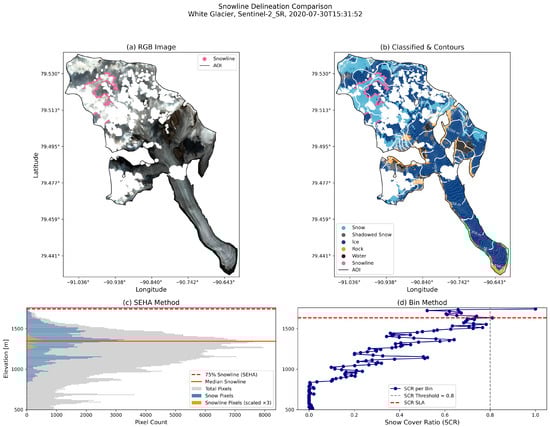
Figure 7. Snowline-altitude retrieval for White Glacier using a Sentinel-2 surface reflectance (SR) scene acquired on 30 July 2020. (a) True-color RGB composite with the automated snowline (magenta) and area-of-interest (AOI) boundary (black). (b) Classified image showing snow (light blue), shadowed snow, bare ice, rock, and water; orange contours indicate elevation intervals. (c) Output from the snowline-elevation histogram analysis (SEHA) method: stacked histograms of total pixels (grey), snow pixels (blue), and snowline pixels (orange, scaled by a factor of 3). The dashed red line marks the 75% cumulative snow frequency, and the solid red line indicates the SEHA-derived snowline. (d) Elevation-bin method showing snow cover ratio (SCR) per 10 m elevation bin (blue points); the SCR threshold of 0.8 is indicated by a dashed grey line, and the derived snowline altitude (SLA) is marked by a horizontal red line. Void regions in the accumulation zone result in upward bias of ~200 m in the bin method and a downward bias of ~80 m in the SEHA method due to differing sensitivities to data voids.

These results highlight a trade-off intrinsic to SLA monitoring. Relaxing AOI-completeness criteria increases temporal sampling and improves detection of transient melt events, but each additional scene with incomplete spatial coverage can non-linearly amplify classification errors in elevation-bin algorithms. For White Glacier, the reduction in spatial data integrity offset the benefits of higher temporal resolution, lowering SLA accuracy.

In temperate or mid-latitude glacier settings, where persistent maritime cloud cover and complex topography frequently limit acquisition, relaxing AOI thresholds may be a necessary compromise. This was evident for Turner Glacier, where increased scene availability improved temporal coverage, yet extensive terrain and cloud shadows obscured large portions of the study area (Figure 8). In such contexts, robust void-handling strategies are required to mitigate classification uncertainty and to ensure reliable SLA estimation under sub-optimal imaging conditions.

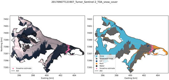
Figure 8. Snow and ice classification results on Turner Glacier based on Sentinel-2 top-of-atmosphere (TOA) imagery acquired on 7 September 2017. (Left) True color composite with snowline estimate. (Right) Classified map showing snow, ice, shadowed snow, rock, and water, with snowline estimate indicated. Note the significant impact of terrain shadow and cloud shadow on classification accuracy.

Another potential source of uncertainty in this methodology arises from the temporal discrepancy between the ArcticDEM epoch (2007–2017) and the more recent satellite imagery (2018–2024). Given the rapid negative surface mass balance and accelerating thinning rates characteristic of Arctic amplification, estimated between 0.5 and 1.0 m yr⁻¹ in recent decades [2,3], the application of a static DEM may introduce a systematic overestimation of absolute SLA as the glacier hypsometry evolves. Nevertheless, validation at White Glacier demonstrates that interannual variability is captured with high fidelity. This suggests that the elevation-binning approach remains a robust proxy for relative SLA fluctuations, particularly in regions where time-resolved topographic data are unavailable.

In summary, while the strict full-coverage protocol in Cheung and Thomson [18] remains the most accurate approach for SLA retrieval from Sentinel-2 SR data, its restrictiveness limits temporal resolution in persistently cloudy Arctic conditions. Relaxing AOI constraints permits a denser seasonal sampling frequency, provided these extractions are integrated with quality-controlled post-processing routines to mitigate potential spatial sampling biases.

6.4. On Extending SLA/ELA Reconstructions with Landsat

With the advent of Sentinel-2 (S2A in 2015; S2B in 2017), many SLA and snow-cover studies have shifted to Sentinel-2 because its 10 m visible/NIR bands, 20 m SWIR bands, and ~5 d revisit markedly improve late-summer clear-sky sampling and reduce mixed-pixel bias at the snow–ice boundary [37,38]. This chapter follows that practice for cross-site comparability and temporal density. In principle, a back-extension using Landsat—Thematic Mapper (TM), Enhanced Thematic Mapper Plus (ETM+), and Operational Land Imager (OLI)—could lengthen the record to 1984; however, it was not implemented here for reliability and scope reasons specific to the study glaciers.

First, the 30 m Landsat pixel size increases mixed-pixel contamination near narrow accumulation zones and steep hypsometry, biasing NDSI mapping and perturbing the elevation-bin snow-cover ratios that underpin SLA estimates (e.g., [39]). Second, Landsat-7 has acquired scan-line corrector (SLC)-off data since 31 May 2003, leaving ~22% wedge-shaped gaps per scene; gap-filling is possible but introduces scene-dependent uncertainties that require quantification for each glacier and year. Third, at High-Arctic latitudes, low solar elevation and frequent cloud/topographic shadow further reduce the number of late-summer, gap-free observations suitable for SLA retrieval, increasing the need for aggressive quality assurance (QA) and per-scene void handling.

Landsat-based SLA/ELA reconstructions are feasible at scale when tailored quality control and harmonisation are applied (e.g., Arctic-wide SLAs from 1984–2022) [10]. Notably, Larocca et al. [10] delineated SLAs by manual interpretation rather than machine-learning classification. Recent work also shows that augmenting raw NDSI with elevation and seasonality covariates can mitigate some Landsat limitations [40,41]. Consistent with these findings, a constrained back-extension is most defensible on wide, high-relief glaciers (broad accumulation zones; lower mixed-pixel risk). Accordingly, a Landsat back-extension is recommended as targeted future work: focus on large basins, implement sensor-specific calibration, and validate against all available field ELA before merging with the Sentinel-2 era.

6.5. Classification Accuracy and Regional Adaptation

Training datasets derived from outside the CAA can introduce substantial uncertainty in per-pixel classification of snow and ice. These uncertainties arise from the distinct physical and spectral characteristics of Arctic glaciers relative to temperate and alpine settings. Accurate separation of snow, ice, and debris-covered surfaces is essential for robust estimates of SCA and SLA; classification errors at this foundational stage propagate through subsequent analyses and degrade downstream metrics.

Visual comparison of classified outputs with true-color composites in this study indicates generally strong separation of snow, shadow, and ground classes. Nevertheless, glacier-specific surface conditions remain challenging for transferable algorithms. Turner Glacier (Figure 9), surveyed in August 2024 by C. Gorwill, provides a salient example: extensive supraglacial debris, comprising mineral dust, ash, and microbial/algal assemblages, lowers albedo and alters the spectral signature of ice, complicating automated delineation and potentially biasing models trained in less debris-rich environments [42].

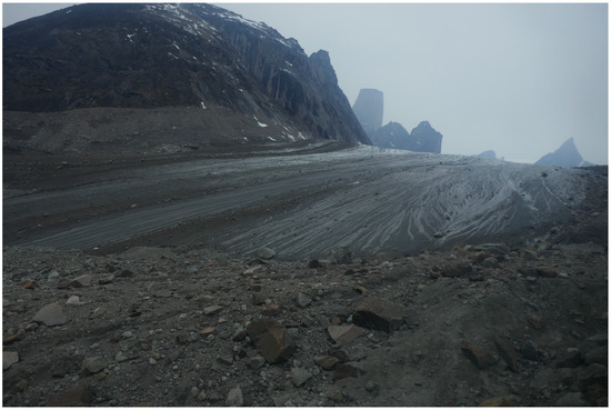
Figure 9. Field photo of Turner Glacier, Baffin Island, taken in August 2024. Extensive supraglacial debris obscures the underlying ice, forming a low-albedo surface that complicates spectral classification. Photo credit: C. Gorwill.

Region-specific effects are further compounded by local lithological diversity. On Bylot Island, glaciers entrain debris from multiple bedrock units, producing spatially heterogeneous surface materials with variable reflectance. Classifiers trained over spectrally uniform terrain—typical of some mid-latitude or monolithic geological settings—may therefore misidentify snow and ice where dark, debris-covered firn is prevalent on Baffin Island [43].

To mitigate these issues, hierarchical classification frameworks have shown promise. As outlined by Prieur et al. [19], a multi-stage architecture that first segregates glaciated surfaces from surrounding terrain and then separates snow from ice can enhance fidelity and improve model transferability. Such tiered approaches reduce misclassification in complex conditions, including shadowed zones and debris-covered ablation areas, and are particularly valuable for SLA estimation on glaciers such as Highway and Coronation, where supraglacial debris and variable illumination increase spectral ambiguity.

6.6. Future Work and Limitations

The reliance on optical multispectral imagery remains a primary limitation due to persistent cloud cover in the High Arctic. Future iterations of this workflow will benefit from transitioning to next-generation cloud masking products available in the GEE catalog, such as GOOGLE/CLOUD_SCORE_PLUS/V1/S2_HARMONIZED or COPERNICUS/S2_CLOUD_PROBABILITY. Preliminary verification indicates that these advanced masks provide superior discrimination between clouds and snow/ice compared to standard bitmasks, which would further enhance data throughput and reduce the inclusion of artifacts in the SCR process.

Furthermore, the integration of Synthetic Aperture Radar (SAR) data, such as those from the Sentinel-1 or RADARSAT Constellation Missions, should be explored. Unlike optical sensors, SAR facilitates penetration of cloud cover and is highly sensitive to the liquid water content of the snowpack, rendering it an effective tool for mapping the SLA during the peak melt season.

However, the application of SAR in the High Arctic is constrained by signal penetration depth, which is highly sensitive to seasonal variations in snow moisture and density. This physical variability introduces significant noise into machine learning training sets, complicating the achievement of the facies-classification accuracy required for reliable SLA retrieval. Nevertheless, forthcoming satellite missions are expected to significantly enhance regional monitoring capabilities. Specifically, the deployment of high-revisit, fully polarimetric SAR constellations and the NASA-ISRO SAR (NISAR) mission will provide the dual-frequency (L- and S-band) data necessary to better distinguish between surface and subsurface snow facies. These advancements will likely facilitate the development of robust multimodal machine learning models, ultimately improving the temporal density of ELA proxies and reducing the uncertainties associated with persistent cloud cover in the CAA.

7. Conclusions

Using 9900 optical scenes from Landsat 8/9 and Sentinel–2, we developed the first decadal (2013–2024) record of late-summer snowline altitude (SLA) for six glaciers located in Auyuittuq and Sirmilik National Parks and on Axel Heiberg Island. A scalable workflow, combining sensor-specific supervised classification, elevation binning of snow-cover ratio (SCR), and a histogram-based method (SEHA: snowline estimation via histogram analysis), enabled consistent SLA retrievals across sites with contrasting hypsometry, cloudiness, and surface characteristics. ArcticDEM v3 provided topographic reference data, and station observations from Pangnirtung, Pond Inlet, and Eureka offered independent thermal forcing metrics in the form of positive degree days (PDD).

Three principal signals emerge from the analysis. First, all glaciers exhibit the canonical seasonal cycle in snow-covered area (SCA): maximum extents in June, minima in August, and partial recovery in September. The amplitude of this cycle increases from the High Arctic (White Glacier) to the more maritime Baffin sector, with widespread minima in 2020. Second, interannual peak SLA correlates with summer thermal conditions. SLA increases with PDD at most sites, with glacier-specific sensitivities of 2.6, 0.7, and 0.8 m °C⁻¹ day⁻¹ for White, Highway, and Turner glaciers, respectively—consistent with enhanced ablation during warm summers. Third, hypsometry modulates glacier vulnerability. Glaciers with limited high-elevation terrain (e.g., Turner Glacier and BylotD20s) regularly lose their accumulation zones in warm years, whereas those with extensive high-relief terrain (e.g., Coronation and Highway glaciers) retain late-summer snow cover despite their more southerly locations.

Method intercomparison and validation against field-derived equilibrium-line altitude (ELA) on White Glacier indicate that the elevation-bin method provides more accurate and temporally responsive SLA estimates than SEHA. The binning method shows lower mean bias (+53 m) and root-mean-square error (RMSE = 177 m) relative to field ELA, compared with SEHA (mean bias +165 m; RMSE = 339 m). Across all sites, SLA estimates from binning are systematically higher than those from SEHA (median offset: 164 m), due to stricter SCR thresholds and reduced influence from non-glacier pixels. Residual differences between SLA and ELA primarily reflect image acquisition timing near the seasonal snow minimum and mixed-pixel effects at the firn–bare-ice boundary.

Our results indicate that a regionally calibrated elevation-bin method, validated against the benchmark record of White Glacier, provides an objective and transferable framework for ELA estimation. While further in situ observations across Baffin and Bylot Islands would strengthen regional calibration, the current workflow addresses a critical observational gap by utilizing a method that is resilient to the spatial uncertainties common in Arctic glacier inventories.

The observed glacier behavior is consistent with recent climatic trends. Mean summer (JJA) and winter (DJF) temperatures have increased across the region, with significant warming observed over multi-decadal records at Eureka. Corresponding increases in PDD imply enhanced melt forcing in recent decades. Precipitation trends are spatially heterogeneous and do not display a coherent regional signal. These climate diagnostics support a regional tendency toward higher late-summer snowlines in the southern Canadian Arctic Archipelago.

Uncertainties in SLA estimation arise from: (i) classification transferability under shadow, debris cover, and variable illumination; (ii) sensor resolution (10 m vs. 30 m) and associated mixed-pixel effects; (iii) delineation parameters (thresholds, bin definitions) and scene quality (void fraction, area-of-interest completeness); and (iv) DEM vertical error and temporal misalignment. While formal vertical uncertainty from ArcticDEM (±4 m) and 10 m elevation-bin quantisation is minor, scene-dependent factors—particularly void fraction—can degrade SLA precision. Notably, increasing temporal sampling by relaxing AOI completeness improves seasonal coverage but also amplifies SLA sensitivity to void artefacts, particularly during cloudy or extreme-melt conditions. These trade-offs should be explicitly considered in future monitoring frameworks.

In summary, this study addresses a critical observational gap for glaciers in the southern Canadian Arctic Archipelago, evaluates the performance of automated SLA methods, and provides a transferable workflow for generating uncertainty-aware SLA time series. Continued Arctic warming and rising PDD underscore the importance of sustained, calibrated SLA monitoring for assessing changes in accumulation-area extent, glacier mass-balance resilience, freshwater resources, and downstream ecosystem services.

References

- Gardner, A.S.; Moholdt, G.; Wouters, B.; Wolken, G.J.; Burgess, D.O.; Sharp, M.J.; Cogley, J.G.; Braun, C.; Labine, C. Sharply increased mass loss from glaciers and ice caps in the Canadian Arctic Archipelago. Nature 2011, 473, 357–360. [Google Scholar] [CrossRef]
- Noël, B.; van de Berg, W.J.; Lhermitte, S.; Wouters, B.; Schaffer, N.; van den Broeke, M.R. Six decades of glacial mass loss in the Canadian Arctic Archipelago. J. Geophys. Res. Earth Surf. 2018, 123, 1430–1449. [Google Scholar] [CrossRef]
- Hugonnet, R.; McNabb, R.; Berthier, E.; Menounos, B.; Nuth, C.; Girod, L.; Farinotti, D.; Huss, M.; Dussaillant, I.; Brun, F.; et al. Accelerated global glacier mass loss in the early twenty-first century. Nature 2021, 592, 726–731. [Google Scholar] [CrossRef] [PubMed]
- Pfeffer, W.T.; Arendt, A.A.; Bliss, A.; Bolch, T.; Cogley, J.G.; Gardner, A.S.; Hagen, J.-O.; Hock, R.; Kaser, G.; Kienholz, C.; et al. The Randolph Glacier Inventory: A Globally Complete Inventory of Glaciers. J. Glaciol. 2014, 60, 537–552. [Google Scholar] [CrossRef]
- Howell, S.; Brady, M. Increased Arctic Ocean sea ice loss through the Canadian Arctic Archipelago under a warmer climate. In Proceedings of the EGU General Assembly 2020, Virtual Event, 4–8 May 2020. [Google Scholar] [CrossRef]
- Environment and Climate Change Canada. Temperature Change in Canada. Canadian Environmental Sustainability Indicators. 2024. Available online: https://www.canada.ca/en/environment-climate-change/services/environmental-indicators/temperature-change.html (accessed on 5 August 2025).
- Intergovernmental Panel on Climate Change. Climate Change 2021: The Physical Science Basis. Working Group I Contribution to the Sixth Assessment Report of the Intergovernmental Panel on Climate Change; Cambridge University Press: Cambridge, UK, 2023. [Google Scholar] [CrossRef]
- Zemp, M.; Hoelzle, M.; Haeberli, W. Six Decades of Glacier Mass-Balance Observations: A Review of the Worldwide Monitoring Network. Ann. Glaciol. 2009, 50, 101–111. [Google Scholar] [CrossRef]
- Goosse, H.; Kay, J.E.; Armour, K.C.; Bodas-Salcedo, A.; Chepfer, H.; Docquier, D.; Jonko, A.; Kushner, P.J.; Lecomte, O.; Massonnet, F.; et al. Quantifying climate feedbacks in polar regions. Nat. Commun. 2018, 9, 1919. [Google Scholar] [CrossRef] [PubMed]
- Larocca, L.J.; Lea, J.M.; Erb, M.P.; McKay, N.P.; Phillips, M.; Lamantia, K.A.; Kaufman, D.S. Arctic glacier snowline altitudes rise 150 m over the last 4 decades. Cryosphere 2024, 18, 3591–3611. [Google Scholar] [CrossRef]
- Koerner, R.M. Mass balance of glaciers in the Queen Elizabeth Islands, Nunavut, Canada. Ann. Glaciol. 2005, 42, 417–423. [Google Scholar] [CrossRef]
- Thomson, L.I.; Copland, L. Glacier Change on Axel Heiberg Island, Nunavut, Canada. J. Glaciol. 2011, 57, 1079–1086. [Google Scholar] [CrossRef]
- Parkes, D.; Goosse, H. Modelling regional glacier length changes over the last millennium using the Open Global Glacier Model. Cryosphere 2020, 14, 3135–3153. [Google Scholar] [CrossRef]
- Rabatel, A.; Bermejo, A.; Loarte, E.; Soruco, A.; Gomez, J.; Leonardini, G.; Vincent, C.; Sicart, J.E. Can the snowline be used as an indicator of the equilibrium line and mass balance for glaciers in the Outer Tropics? J. Glaciol. 2012, 58, 1027–1036. [Google Scholar] [CrossRef]
- Rastner, P.; Prinz, R.; Notarnicola, C.; Nicholson, L.; Sailer, R.; Schwaizer, G.; Paul, F. On the Automated Mapping of Snow Cover on Glaciers and Calculation of Snow Line Altitudes from Multi-Temporal Landsat Data. Remote Sens. 2019, 11, 1410. [Google Scholar] [CrossRef]
- Yue, X.; Li, Z.; Zhao, J.; Li, H.; Wang, P.; Wang, L. Changes in the end-of-summer snow line altitude of summer-accumulation-type glaciers in the Eastern Tien Shan Mountains from 1994 to 2016. Remote Sens. 2021, 13, 1080. [Google Scholar] [CrossRef]
- Li, X.; Wang, N.; Wu, Y. Automated glacier snow line altitude calculation method using Landsat series images in the Google Earth Engine platform. Remote Sens. 2022, 14, 2377. [Google Scholar] [CrossRef]
- Cheung, W.Y.; Thomson, L. Using K-Means-derived pseudo-labels and machine learning classification on Sentinel-2 imagery to delineate snow cover ratio and snowline altitude: A case study on White Glacier from 2019 to 2024. Remote Sens. 2025, 17, 3872. [Google Scholar] [CrossRef]
- Prieur, C.; Rabatel, A.; Thomas, J.B.; Farup, I.; Chanussot, J. Machine learning approaches to automatically detect glacier snow lines on multi-spectral satellite images. Remote Sens. 2022, 14, 3868. [Google Scholar] [CrossRef]
- Aberle, R.; Enderlin, E.; O’Neel, S.; Florentine, C.; Sass, L.; Dickson, A.; Marshall, H.P.; Flores, A. Automated snow cover detection on mountain glaciers using space-borne imagery. EGUsphere 2024, 2024, 1–28. [Google Scholar] [CrossRef]
- Cheung, W.Y. Decadal Glacier Geometry and Mass Changes in Auyuittuq and Sirmilik National Parks, Canadian Arctic (1958–2024). Ph.D. Thesis, Queen’s University, Kingston, ON, Canada, 2025. [Google Scholar]
- Syvitski, J.P.M. Glaciomarine environments in Canada: An overview. Can. J. Earth Sci. 1993, 30, 354–371. [Google Scholar] [CrossRef]
- Pelto, M. Coronation Glacier: New Island Development, Baffin Island. GlacierChange Blog. 2023. Available online: https://glacierchange.blog/2023/10/11/coronation-glacier-new-island-development-baffin-island/ (accessed on 17 April 2025).
- Dowdeswell, E.K.; Dowdeswell, J.A.; Cawkwell, F. On the glaciers of Bylot Island, Nunavut, Arctic Canada. Arct. Antarct. Alp. Res. 2007, 39, 402–411. [Google Scholar] [CrossRef]
- Wainstein, P.A.; Moorman, B.J.; Whitehead, K. Glacial conditions that contribute to the regeneration of Fountain Glacier proglacial icing, Bylot Island, Canada. Hydrol. Process. 2014, 28, 2749–2760. [Google Scholar] [CrossRef]
- World Glacier Monitoring Service. White Glacier. WGMS Reference Glaciers Database. 2023. Available online: https://wgms.ch/products_ref_glaciers/ (accessed on 3 February 2025).
- GLIMS Consortium. GLIMS Glacier Database, Version 1; [Dataset]; National Snow and Ice Data Center: Boulder, CO, USA, 2016. [CrossRef]
- Porter, C.; Howat, I.; Noh, M.J.; Husby, E.; Khuvis, S.; Danish, E.; Tomko, K.; Gardiner, J.; Negrete, A.; Yadav, B.; et al. ArcticDEM—Mosaics, Version 4.1. [Dataset]. Harvard Dataverse. 2023. Available online: https://dataverse.harvard.edu/dataset.xhtml?persistentId=doi:10.7910/DVN/3VDC4W (accessed on 1 February 2025).
- Porter, C.; Morin, P.; Howat, I.; Noh, M.J.; Bates, B.; Peterman, K.; Keesey, S.; Schlenk, M.; Gardiner, J.; Tomko, K.; et al. ArcticDEM, Version 3. [Dataset]. Harvard Dataverse. 2018. Available online: https://dataverse.harvard.edu/dataset.xhtml?persistentId=doi:10.7910/DVN/OHHUKH (accessed on 1 February 2025).
- Hall, D.K.; Riggs, G.A.; Salomonson, V.V. Development of methods for mapping global snow cover using Moderate Resolution Imaging Spectroradiometer data. Remote Sens. Environ. 1995, 54, 127–140. [Google Scholar] [CrossRef]
- Guo, Z.; Wang, N.; Shen, B.; Gu, Z.; Wu, Y.; Chen, A. Recent spatiotemporal trends in glacier snowline altitude at the end of the melt season in the Qilian Mountains, China. Remote Sens. 2021, 13, 4935. [Google Scholar] [CrossRef]
- Tepes, P.; Gourmelen, N.; Nienow, P.; Tsamados, M.; Shepherd, A.; Weissgerber, F. Changes in elevation and mass of Arctic glaciers and ice caps, 2010–2017. Remote Sens. Environ. 2021, 261, 112481. [Google Scholar] [CrossRef]
- Wójcik, K.A.; Sobota, I. Spatial and temporal changes in ablation, distribution and evolution of glacial zones on Irenebreen, a small glacier of the high Arctic, Svalbard. Polar Sci. 2020, 23, 100503. [Google Scholar] [CrossRef]
- Conway, J.P.; Cullen, N.J. Cloud effects on surface energy and mass balance in the ablation area of Brewster Glacier, New Zealand. Cryosphere 2016, 10, 313–328. [Google Scholar] [CrossRef]
- Conway, J.P.; Abermann, J.; Andreassen, L.M.; Azam, M.F.; Cullen, N.J.; Fitzpatrick, N.; Giesen, R.H.; Langley, K.; MacDonell, S.; Mölg, T.; et al. Cloud forcing of surface energy balance from in situ measurements in diverse mountain glacier environments. Cryosphere 2022, 16, 3331–3356. [Google Scholar] [CrossRef]
- Curley, A.N.; Kochtitzky, W.H.; Edwards, B.R.; Copland, L. Glacier changes over the past 144 years at Alexandra Fiord, Ellesmere Island, Canada. J. Glaciol. 2021, 67, 511–522. [Google Scholar] [CrossRef]
- Drusch, M.; Del Bello, U.; Carlier, S.; Colin, O.; Fernandez, V.; Gascon, F.; Hoersch, B.; Isola, C.; Laberinti, P.; Martimort, P.; et al. Sentinel-2: ESA’s optical high-resolution mission for GMES operational services. Remote Sens. Environ. 2012, 120, 25–36. [Google Scholar] [CrossRef]
- Gascoin, S.; Barrou Dumont, Z.; Deschamps-Berger, C.; Marti, F.; Salgues, G.; López-Moreno, J.I.; Revuelto, J.; Michon, T.; Schattan, P.; Hagolle, O. Estimating fractional snow cover in open terrain from Sentinel-2 using the Normalized Difference Snow Index. Remote Sens. 2020, 12, 2904. [Google Scholar] [CrossRef]
- Xiao, X.; Liang, S. Assessment of snow cover mapping algorithms from Landsat surface reflectance data and application to automated snowline delineation. Remote Sens. Environ. 2024, 307, 114163. [Google Scholar] [CrossRef]
- Poussin, C.; Timoner, P.; Chatenoux, B.; Giuliani, G.; Peduzzi, P. Improved Landsat-based snow cover mapping accuracy using a spatiotemporal NDSI and generalized linear mixed model. Sci. Remote Sens. 2023, 7, 100078. [Google Scholar] [CrossRef]
- Poussin, C.; Peduzzi, P.; Giuliani, G. Snow observation from space: An approach to improving snow cover detection using four decades of Landsat and Sentinel-2 imageries across Switzerland. Sci. Remote Sens. 2025, 11, 100182. [Google Scholar] [CrossRef]
- Gorwill, C. Ice Darkening on Turner Glacier in Auyuittuq National Park, Nunavut. Master’s Thesis, Queen’s University, Kingston, ON, Canada, 2024. [Google Scholar] [CrossRef]
- DiLabio, R.N.W.; Shilts, W.W. Composition and Dispersal of Debris by Modern Glaciers, Bylot Island, Canada. In Moraines and Varves; Balkema: Rotterdam, The Netherlands, 1979; pp. 146–155. [Google Scholar]
Disclaimer/Publisher’s Note: The statements, opinions and data contained in all publications are solely those of the individual author(s) and contributor(s) and not of MDPI and/or the editor(s). MDPI and/or the editor(s) disclaim responsibility for any injury to people or property resulting from any ideas, methods, instructions or products referred to in the content. |
© 2026 by the authors. Licensee MDPI, Basel, Switzerland. This article is an open access article distributed under the terms and conditions of the Creative Commons Attribution (CC BY) license.