Highlights
What are the main findings?
- An integrated satellite and UAV remote sensing approach revealed the spatial and temporal characteristics of the suspended sediment plume phenomenon, known as the Ieodo plume.
- A physical generation mechanism for the Ieodo plume was demonstrated, based on the synthesis of the remote sensing results.
What are the implications of the main findings?
- The Ieodo plume is a physical oceanographic phenomenon initially governed by tidal-driven momentum and subsequently by buoyancy and inertia.
- A combined satellite–UAV observational framework can substantially improve the monitoring and quantification of rapidly evolving submesoscale turbidity events.
Abstract
The Ieodo plume is a distinctive suspended sediment plume near the Ieodo Ocean Research Station (I-ORS), located in the middle of the northern East China Sea. Because the Ieodo plume exhibits multiple different spatial scales, this study conducted an integrated remote sensing observation using satellites and unmanned aerial vehicles (UAVs) to observe its development and dispersion. Sentinel-2 and Geostationary Ocean Color Imager-II (GOCI-II) data were used to determine the plume’s spatial characteristics, broad-scale behavior, hourly variability, and turbidity characteristics. Also, TPXO model outputs were employed to evaluate the relationship between plume occurrence and tides, together with satellite imagery. Plume was repeatedly observed near the top of the Ieodo Seamount, with an affected extent of 11.4 ± 3.2 km in the east–west direction and 14.3 ± 4.1 km in the north–south direction. Moreover, hourly variations observed using GOCI-II showed that the Ieodo plume rotated clockwise with shifting tidal currents, forming a counterclockwise curved band or a ring-shaped structure. Total suspended solids (TSSs) in the plume reached their maximum when the southward component of the TPXO tidal current was dominant. Based on UAV optical surveys at the I-ORS, fine-scale morphology at the early stage of plume development was revealed, and it was confirmed that the Ieodo plume can occur even when it is not detected by satellite imagery. Furthermore, the u- and v-velocity vectors of the propagating Ieodo plume were derived by applying large-scale particle image velocimetry (LSPIV) to geometrically corrected sequential UAV imagery obtained in I-ORS. Plume speed was greatest near the source during the initial stage (0.81 ± 0.30 m s−1) and gradually decreased to 0.34 ± 0.29 m s−1 over distance. Based on the results above, we propose that the Ieodo plume is primarily generated by a pressure reduction associated with tidally accelerated currents over topography, driven by the Bernoulli effect. This study shows that an integrated satellite and UAV observation framework can effectively monitor rapidly evolving suspended sediment plumes. It can further help improve our understanding of dynamically driven submesoscale marine events.
1. Introduction
Sediment plumes occurring in the ocean are known to increase seawater turbidity, thereby reducing sunlight entering the ocean, and to adsorb contaminants such as heavy metals, enabling their transport over long distances [1,2,3]. Following deposition, they are also considered highly significant in marine environmental research because the decomposition of organic matter within sediments increases sediment oxygen demand (SOD), depletes bottom-water oxygen, and exerts physical and chemical impacts on benthic ecosystems [4,5,6,7,8]. In the ocean, sediments are primarily resuspended when bottom shear stress induced by strong tidal currents or waves exceeds a critical threshold [9,10] or when episodic turbulence events occur [11,12]. Accordingly, previous discussions have focused mainly on high-velocity environments such as estuaries and on shallow coastal regions [13,14,15,16], as well as on settings susceptible to anthropogenic disturbances, including dredging and mining activities [5,17,18].
The dynamics and dispersion of these marine suspended sediment plumes have been studied primarily through (1) theoretical approaches, (2) numerical models, and (3) remote sensing observations and in situ measurements. Theoretical studies based on the classical turbulent plume theory assume that the plume radius originating from a point or line source grows linearly and interpret plume evolution using governing equations that incorporate factors such as volume flux, momentum flux, and buoyancy flux [19,20,21]. Numerical modeling aims to simulate the spatiotemporal evolution of plumes and to predict their future states by combining background flows such as tides, winds, and coastal currents and key processes, including particle settling and resuspension [22,23,24]. In remote sensing, satellite imagery from ocean-color and optical sensors is commonly used to derive turbidity or suspended sediment concentrations, thereby enabling analysis of plume distribution and behavior over broad scales [15,16,25,26,27,28,29,30]. For field data, in coastal regions, sensors such as turbidimeters and current meters are used to investigate the concentration and spatial extent of the plume, along with water samples obtained in situ [25,31]. In the case of the mid- to near-bottom plumes in the deep sea, moorings, autonomous underwater vehicles (AUVs), and remotely operated vehicles (ROVs) are commonly used to examine the structure and redeposition characteristics of the plume [18,32,33,34].
Suspended sediment plumes that occur in estuarine and coastal environments form close to the shoreline and exhibit a distinct turbid water signal, which reaches the sea surface and makes them readily observable on satellite and airborne platforms. However, because these plumes arise in settings where multiple factors interact, such as river discharge, tides, coastal currents, wind-driven vertical mixing, and adjacent coastal topography, it is difficult to distinguish the contributions of external forcing factors throughout plume formation, development, and decay. Moreover, interpreting plume dispersion and morphological evolution using only a small number of dominant drivers entails substantial uncertainty. In contrast, suspended sediment plumes in the deep sea have been examined mainly in association with mining activities, typically at depths greater than 1000 m. Because fewer external forcing factors influence them, their flow fields are relatively simple compared to those in coastal settings [18,33]. Accordingly, they are well-suited for examining the principles governing plume formation and dispersion from both theoretical and numerical modeling perspectives. However, because deep-sea suspended sediment plumes generally remain in the mid- to near-bottom layers after initiation and in most cases do not reach the surface, their behavior cannot be readily characterized directly through remote sensing; thus, observations are constrained by a heavy reliance on instruments such as AUVs and ROVs and on numerical models.
Distinct from both coastal and deep-sea plumes, a suspended sediment plume phenomenon known as the Ieodo plume (Figure 1) occurs in the vicinity of the Ieodo Ocean Research Station (I-ORS), located in the northern East China Sea. Although the Ieodo plume forms in an offshore environment, it displays a distinctive feature similar to estuarine and coastal suspended sediment plumes, where resuspended sediments reach the surface and subsequently disperse laterally. These traits make the Ieodo plume easy to detect via remote sensing observations, as in coastal and estuarine plumes, while retaining a relatively simple forcing structure comparable to that of deep-sea plumes. Nevertheless, owing to limited access to the source region and a lack of long-term, wide-area surveys, the Ieodo plume is not sufficiently understood, with only a few reports of its occurrence; its specific generation mechanisms and dynamical characteristics also remain unclear.
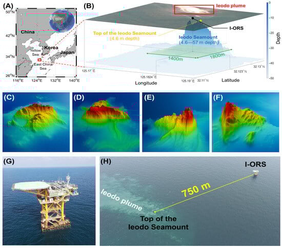
Figure 1.
(A) Location of the Ieodo region. (B) Schematic of the Ieodo Seamount and the Ieodo plume. (C–F) Views of the Ieodo Seamount from the north, south, west, and east, respectively. (G) Ieodo Ocean Research Station (I-ORS). (H) Distance between I-ORS and the Ieodo plume source area.
Because the Ieodo plume occurs in offshore regions with limited accessibility, and its physical characteristics are not yet well understood, satellite remote sensing is a practical primary approach among the three methods mentioned earlier. However, the spatiotemporal resolution of optical satellite data is insufficient for monitoring rapidly evolving physical marine processes, such as plumes. Thus, it remains challenging to characterize plume dynamics, dispersal patterns, and spatial coverage using satellite remote sensing alone. To address these limitations, we employed an integrated framework that combines satellite-based remote sensing with high-resolution unmanned aerial vehicle (UAV) observations. Low-altitude remote sensing using UAVs can effectively capture fine-scale morphological changes and short-term plume movements through continuous, high-resolution imagery.
We analyzed Sentinel-2A/2B and Geostationary Ocean Color Imager-II (GOCI-II) satellite data to identify the overall size and morphology of the developed Ieodo plume and its source region. In particular, we examined the plume turbidity and its temporal variability using total suspended solids (TSS) products from GOCI-II, which provides time-resolved observations. In addition, high-resolution optical data were collected at the I-ORS using UAVs to document the aggregate structure of the sediments during the initial stage of plume formation and to resolve the early dispersal pattern. Furthermore, subsurface plume signatures were also captured using UAV imagery, which were not readily detectable by satellite sensors. Simultaneously, seawater samples from the plume were collected using a custom-built UAV-based water sampler during plume occurrence to quantify the TSS concentration. Moreover, using large-scale particle image velocimetry (LSPIV), seawater flow fields near the plume-generation site were derived from UAV optical sensor imagery.
By synthesizing the results of this integrated remote sensing approach, a scenario for the generation and dispersion of the Ieodo plume was proposed. These findings are expected to be applicable to the analysis and prediction of plume behavior in river estuaries and coastal waters, as well as to suspended sediment dynamics arising from seabed resource extraction and dredging activities.
To clearly state the scope of this work, the objective of this study is to analyze the Ieodo plume’s dispersal and its morphological and dynamical characteristics using an integrated approach combining satellite observations and UAV measurements. To achieve the research goal, we conducted the following processes: (1) We conceptualize the Ieodo plume as a distinct offshore suspended sediment plume type that is readily observable at the surface yet driven by a comparatively simpler forcing structure, and (2) we propose the Ieodo plume’s generation and dispersion scenario based on integrated satellite–UAV analyses, supported by in situ TSS sampling and LSPIV-derived surface currents.
2. Materials and Methods
2.1. Study Area
The Ieodo Seamount, where the Ieodo plume occurs, is located in the northern East China Sea (Figure 1A). The northern East China Sea is a flat continental shelf region dominated by tidal currents, specifically characterized by the predominance of the semidiurnal M2 constituent and pronounced diurnal tidal inequality [26,29,30]. The maximum surface current speed is relatively high, reaching 0.98–1.4 m s−1 [35]. The Ieodo Seamount spans approximately 1.4 km × 1.8 km, and the depth is shallow at 4.6 m at the summit, while the maximum water depth is 57 m (Figure 1B). Figure 1C–F show the topography of the Ieodo Seamount with high-resolution digital elevation model (DEM) data (1-m spatial resolution) from the north, south, west, and east perspectives, respectively. The seamount has steep slopes, especially in the north–south direction, and a long ridge extending east–west. Notably, several uplifted features are distributed across the northern slope.
The I-ORS, installed in 2003 at a site of approximately 40 m water depth on the southern slope of the seamount, is located at 32°07′22″N, 125°10′56″E, approximately 750 m south of the summit of the Ieodo Seamount located at 32°07′43″N, 125°10′50″E (Figure 1G,H). The I-ORS is highly valuable for marine and meteorological research because it provides real-time observations of diverse variables, including water temperature, salinity, wind, waves, atmospheric pressure, and sea surface height “https://kors.kiost.ac.kr/data/accessData?base=I-ORS (accessed on 2 March 2026)”.
2.2. Satellite Data and Reanalysis Products
To observe the full coverage of the Ieodo plume, we used Sentinel-2A and -2B level-1C (L1C) and level-2A (L2A) products from 2015 to 2024, with a spatial resolution of 10 m × 10 m and a temporal resolution of five days “https://browser.dataspace.copernicus.eu/ (accessed on 2 March 2026)”. Among images with a cloud cover of 10% or less, we collected satellite data for scenes that include the longitude and latitude coordinates of the I-ORS. For plume identification, we primarily used atmospherically corrected L2A products, which were partially supplemented with L1C imagery for several dates when L2A data were unavailable over the Ieodo region. Using the Sentinel Application Platform (SNAP; v10.0.0), we generated true-color RGB images with B2 (490 nm), B3 (560 nm), and B4 (665 nm) assigned to blue, green, and red, respectively, to verify the presence of the Ieodo plume. Quantitative analysis of plume characteristics, including plume size and initial plume width, was conducted using QGIS (v.3.40.4), a geographic information system (GIS) software. The WGS 84 (EPSG:4326) coordinate system was used to display satellite imagery to identify the location of the Ieodo plume. In addition, a distance measurement tool was used to quantify the initial plume width, dispersal extent, and related metrics.
To analyze the hourly behavior of the Ieodo plume and estimate its concentration, we acquired Geostationary Ocean Color Imager-II (GOCI-II) Slot 7 level-1B RGB data and level-2 total suspended solids (TSS) products with a spatial resolution of 250 m × 250 m and a temporal resolution of one day (10 acquisitions at 1 h intervals) “https://www.nosc.go.kr/program/actionGociDownload.do (accessed on 2 March 2026)”. Although GOCI-II data have been available since the second half of 2020, our analysis used data from 22 December 2022, when the provision of hourly level-2 TSS products began, through 2024.
Hourly tidal information for the waters adjacent to Ieodo was obtained from Oregon State University (OSU)’s TPXO8-atlas30 global barotropic tidal atlas model “https://www.tpxo.net/global (accessed on 2 March 2026)”. The TPXO8-atlas30 is a linear barotropic numerical model that incorporates 13 tidal constituents (M2, S2, N2, K2, K1, O1, P1, Q1, M4, MF, MM, MS4, and MN4), provides depth-averaged tidal currents over the East China Sea at a grid spacing of 1/30°, and includes data assimilation. The key specifications of the satellite products and the tidal model used in this study are summarized in Table 1.

Table 1.
Satellite- and reanalysis-based datasets used in this study.
2.3. Low-Altitude Remote Sensing
2.3.1. Field Observations
To examine the initial morphology and fine-scale dynamics of the Ieodo plume, continuous observations were conducted in 2014 at the I-ORS by attaching a GoPro HERO 3+ Black camera to a Skyhook 3.0 helikite and monitoring the plume behavior at its source location [36,37]. In addition, imagery acquired with a DJI Phantom 4 Pro drone during 2019–2021 was used to investigate the plume morphology during the initial generation stage. Subsequently, to continuously observe the plume dispersion from a fixed position and to estimate current velocities during plume occurrence, hovering observations using a DJI Mavic Air 2 platform were performed at the I-ORS from 16 to 18 August 2025. During these observations, a pitch angle of 45° and an azimuth angle of 135° were adopted to minimize the influence of sun glint and cloud shadows [38]. The data were collected at an actual altitude of 237 m by setting the flight altitude to 200 m above the I-ORS helideck, at an elevation of approximately 37 m. Continuous imagery was obtained at 3 s intervals for approximately 5–6 min using the interval shooting mode supported by the DJI Fly application, and the resulting images had a resolution of 12 MP (4000 × 3000 px). The Mavic Air 2 is equipped with a 1/2″ CMOS sensor with dimensions of 6.4 mm × 4.8 mm and a focal length of 4.5 mm. Based on these specifications, the mean ground sampling distance (GSD), which was calculated while accounting for platform altitude and pitch angle, was approximately 28 cm. The specifications of the UAV-borne imaging sensors used for the low-altitude observations are summarized in Table 2.
Table 2.
UAV platforms used for low-altitude observations.
2.3.2. UAV-Based Water Sampling and SPM Analysis
To obtain seawater samples from the locations where the Ieodo plume occurred, we conducted UAV-based water sampling. The traditional, well-established approach to collecting seawater samples is ship-based sampling using devices such as baskets or Niskin bottles [39,40,41]. However, in the Ieodo region, strong currents make it difficult to maintain a fixed position, so the vessel must remain in motion. During such operations, propeller-induced mixing can disturb in situ turbidity measurements. UAV-based sampling has a limited maximum takeoff weight, which restricts the sample volume [42] and, for the same reason, makes it difficult to employ additional weights, thereby constraining sampling to surface waters. Nonetheless, this approach enables accurate sampling at the plume site while minimizing the disturbance associated with mixing. In this study, we collected seawater samples from four different locations within the plume-occurrence area using a UAV-based sampling system in which an approximately 700 mL sampling container was attached via a 10 m line to a DJI Inspire 1 drone (maximum takeoff weight 3500 g; platform weight 2935 g). Prior to sampling, the precise location of the turbid water was identified using an optical camera mounted on the drone. After confirming that the sampling container had contacted the sea surface at the target point, the platform was maneuvered horizontally to tow the container several meters away from the contact point. As some water was lost during the return to the I-ORS, the final collected volume of the samples was approximately 500 mL per flight.
The collected seawater samples were divided into two subsamples per site for analysis of suspended particulate matter (SPM) concentration following a National Institute of Fisheries Science (NIFS) guideline “https://www.nifs.go.kr/distantwater/skin/doc.html?fn=20240125101758566RTU.pdf&rs=/distantwater/preview/Board0052/ (accessed on 2 March 2026)”. The volume of each subsample was set to 250 mL to accommodate field conditions while remaining consistent with the guideline’s intent, with reference to the guidelines for SPM in highly turbid seawater, which specify 300 mL. On the day of sampling, each subsample was filtered through a pre-weighed filter. In this process, an additional 250 mL of tertiary distilled water was filtered to remove potential contaminants and salts from the seawater sample and to lyse the remaining phytoplankton cells via osmotic effects, thereby minimizing the influence of phytoplankton on the SPM analysis. After filtration, the samples were frozen and postprocessed in the laboratory. The filtered papers were dried in an oven at 75 °C for 24 h, a temperature intentionally set relatively low to prevent deformation of the Petri dish during drying, as noted in the referenced guideline; cooled to room temperature in a desiccator; and finally weighed on an electronic balance.
2.3.3. Processing of UAV Imagery: Geometric Correction and PIV-Based Velocity Estimation
In this study, particle image velocimetry (PIV) analysis was performed using sequential UAV optical imagery to estimate current velocities during Ieodo plume events in situations where in situ current-measurement instruments were limited. PIV is a technique that estimates instantaneous particle displacement from a sequence of images acquired by a fixed camera and computes frame-to-frame displacement of particle patterns over an entire interrogation grid to derive a velocity field [43,44]. In particular, PIV applied to imagery with scene scales ranging from a few square meters to several tens of thousands of square meters, as in this study, is referred to as large-scale PIV (LSPIV). This approach has been regarded as a cost-effective and operationally efficient method; therefore, since the 2000s, it has become a standardized non-contact technique for measuring surface flow velocities [45,46,47]. More recently, its integration with UAV platforms has substantially reduced field constraints [48,49]. In general, images of the ocean surface, where distinct particulate tracers are not readily observed, contain numerous noise sources, such as sun glints reflected from the sea surface and whitecaps produced by wave breaking, making it challenging to describe current motion using LSPIV. However, when there is a clear contrast between particles and the surrounding water, and the target particles can function as passive tracers representative of the flow, as in the case of the Ieodo plume, the velocities can be effectively estimated [50,51,52].
Figure 2 illustrates the complete LSPIV workflow implemented in this study using the PIVLab (v3.11) graphical user interface (GUI) within our MATLAB environment (R2024b). To estimate velocities from the UAV-acquired imagery, it is first necessary to orthorectify the original images onto a two-dimensional planar coordinate system through geometric correction. Geometric correction is the process of compensating for geometric distortions in remote sensing imagery such that pixel-based coordinates correspond to real-world geographic coordinates [53,54]. In terrestrial remote sensing, precise geometric corrections are typically performed by using ground control points (GCPs) with known coordinates [50,52]. However, when observing continuously moving fluids, such as rivers and the open ocean, GCP-based approaches are difficult to apply; accordingly, a direct georeferencing approach that assumes the fluid surface to be planar is commonly used [41,51,55,56,57]. In this study, following the approach introduced by Kim et al. [57], direct georeferencing was performed using platform position and attitude information recorded by the onboard Global Positioning System (GPS) and inertial measurement unit (IMU) sensors, respectively. In addition, the actual spatial extent of the imaged area was estimated with the calculated mean GSD.
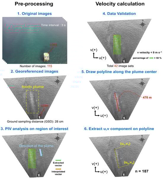
Figure 2.
Overall workflow for estimating Ieodo plume velocities using LSPIV applied to sequential UAV-based optical imagery.
Because trapezoidal images projected onto a plane through geometric correction rely on the mean GSD to estimate the actual lengths and areas of the imaged domain, distortions in length and area increase toward the image margins. Therefore, additional processing is required to minimize these effects. In this study, the distortion effects were limited by defining a region of interest (ROI) that was restricted to the central portion of the image where the Ieodo plume signal was clearly identifiable and by computing particle-based flow fields only within the ROI. Next, all vectors with a positive v-component were removed, because sequential imagery showed that the Ieodo plume propagated distinctly in the negative v-direction. To ensure the robustness of the velocity estimates, in the final processing step, we interpolated only 42 image sets for which the valid detection probability (VDP) of the resulting velocity fields exceeded 50%, following the procedures described above. In particular, even within the ROI, velocities were extracted at 187 points along an approximately 470 m straight transect drawn through the plume core to depict as precisely as possible only the flow attributable to the Ieodo plume as accurately as possible.
2.4. In Situ Data
For the bathymetric analysis of the Ieodo Seamount, we used a high-resolution digital elevation model (DEM) dataset with a spatial resolution of 1 m × 1 m, provided by the Korea Hydrographic and Oceanographic Agency (KHOA). To characterize the depth-dependent water temperature in the Ieodo region during the survey period in August 2025, we used quality-controlled temperature data measured at 10 min intervals with the I-ORS conductivity–temperature–depth (CTD) instrument.
3. Results
3.1. Full-Coverage Observation of the Ieodo Plume
Sentinel-2 satellite data encompassing the Ieodo region were collected from 2015 to 2024 to investigate the spatial characteristics of the Ieodo plume. Around the Sentinel-2 overpass time for the Ieodo area (approximately 11:20, UTC+9), the Ieodo plume was observed in a range of morphologies (Figure 3). In addition, quantitative analyses were conducted in QGIS using satellite-image metadata. Sentinel-2 imagery showed that the Ieodo plume consistently originates from a certain point slightly north of the I-ORS (Figure 3). This site corresponds to the summit of the Ieodo Seamount, where the water depth is shallow (approximately 4.6 m). Given that the plume is consistently generated at this point, regardless of its subsequent dispersal direction, the presence of the Ieodo Seamount and the occurrence of the Ieodo plume appear to be closely linked. After its initiation, the Ieodo plume initially propagated while maintaining a relatively uniform width and then broadened and showed a tendency to curve counterclockwise (Figure 3). Based on analyses of 20 Sentinel-2 scenes in which the ring-like structure of the plume was clearly expressed, the Ieodo plume, which emerged with an initial width of approximately 0.5 km from the source, expanded after full development to extents of 11.4 ± 3.2 km along the x-axis and 14.3 ± 4.1 km along the y-axis. This scale is broadly comparable to that of plumes that typically occur under normal conditions in estuaries and small bays fed by small- to medium-sized rivers [15,58,59,60].
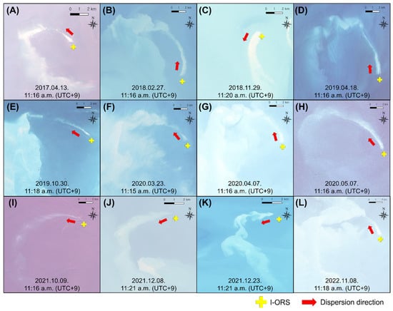
Figure 3.
(A–L) Ieodo plumes identified in RGB composites generated in QGIS from Sentinel-2A/2B’s level 1C bands B2 (490 nm), B3 (560 nm), and B4 (665 nm). The yellow cross and red arrow indicate the I-ORS and plume dispersion direction, respectively. Since radiance varies with acquisition time, all images show different background colors.
Although the 10 m × 10 m spatial resolution of Sentinel-2 imagery enables a relatively detailed description of the developed Ieodo plume, its 5-day temporal resolution and observational gaps due to cloud cover render the data insufficient to elucidate the short-term variability of the plume. Therefore, we used data from the GOCI-II geostationary satellite to characterize the short-term behavior of the plume. Using GOCI-II TSS level 2 data with a spatial resolution of 250 m × 250 m, we analyzed hourly variations in plume shape and sediment concentration from 22 December 2022 to 2024, specifically using data from dates when the Ieodo region was clearly visible in RGB imagery.
Inspection of the GOCI-II TSS products indicated that, in some cases where plume TSS values were low, the boundary between the plume and the surrounding seawater could not be clearly distinguished. Accordingly, this study focused only on Ieodo plume events for which a band- or ring-shaped feature was distinctly observed around the Ieodo summit location and the daily maximum TSS within that area exceeded 10 g m−3. This criterion was adopted because the mean turbidity in the waters surrounding Ieodo is substantially below 10 g m−3 for most of the year [61,62], and this threshold is widely used as a criterion for turbid waters in coral reef management and marine monitoring [63,64,65]. Applying these criteria, 14 events exhibiting a clear contrast with ambient water and a stable hourly configuration were selected for analysis, enabling an examination of the hourly dynamics of the Ieodo plume.
As shown in Figure 4, a distinct clockwise rotation of the plume was observed in all images in which the Ieodo plume occurred. Given that the semidiurnal M2 constituent dominates the northern East China Sea, including the Ieodo area, and that tidal currents rotate clockwise at a rate of approximately 29° per hour to form a tidal ellipse, this result can be interpreted as a phenomenon driven by tidal variations. Indeed, a comparison with hourly TPXO tidal data collected at the same times as the GOCI-II observations showed close agreement between the tidal-current direction and the direction in which the plume was generated from the top of the Ieodo Seamount.
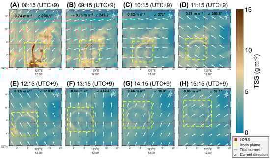
Figure 4.
(A–H) Ieodo plume (yellow boxed area) identified in hourly GOCI-II TSS imagery on 31 October 2023, together with tidal currents from the TPXO8-atlas30 model (white arrows). The yellow box indicates the Ieodo plume. The values in the top-left corner represent the average tidal-current velocities in the areas shown in the satellite imagery.
If the initial flow of the Ieodo plume is governed by tidal forcing, both the counterclockwise-curved plume shape and the clockwise rotation of the plume’s overall band (or ring) structure can be explained simultaneously. Suppose that the source point of plume initiation was fixed and the current direction remained constant without variation. In that case, the plume would advect along an approximately straight trajectory aligned with the current direction. However, in the actual environment, the tidal-current direction changes hourly, rotating clockwise along the tidal ellipse; accordingly, the instantaneous straight-line direction of plume advection from the same source likewise rotates continuously clockwise. Thus, although the plume moves at each moment along a straight path consistent with the contemporaneous tidal-current direction, the direction of the emitted straight-line flow itself rotates clockwise over time. Consequently, the accumulated spatial patterns may be curved counterclockwise. This is similar to the situation in which the nozzle of a hose, rotating clockwise, continuously ejects water from a fixed position. At each moment, the water jet moves forward linearly along the nozzle direction; however, the overall trajectory of the water may appear to curve counterclockwise. Under ideal conditions, the plume can be primarily governed by inertia, leading to a circular, ring-like structure as shown in Figure 4.
However, the clockwise movement of the overall structure of the Ieodo plume, on the other hand, can be explained in terms of the Coriolis force. If the Ieodo plume velocity is set to 0.5 m s−1, the characteristic length scale is set to 10 km, and the Coriolis parameter at 32°N is set to 7.5 × 10⁻⁵ s−1, the Rossby number is calculated using Equation (1).
Because the Rossby number is less than one, the influence of the Coriolis force cannot be readily neglected when interpreting the dynamics of the Ieodo plume. Therefore, even if the plume advects linearly at each moment following the tidal current, the rightward deflection due to the Coriolis force in the Northern Hemisphere can cause the plume to behave as a clockwise-rotating structure.
Among the images acquired on days for which hourly plume behavior could be identified, the time at which the intraday TSS reached its maximum most often coincided with the tidal-current direction being closest to due south (180°). On dates lacking plume observations during southward tidal currents, the highest TSS occurred when the plume advanced toward the westerly direction closest to the south. On 11 of the 14 days, the intraday maximum TSS was within the range of 10–30 g m−3, whereas the highest value identified among the available images was approximately 340 g m−3. The TSS of the plume exhibited a gradual decrease as the plume rotated clockwise on an hourly basis.
Peak TSS concentrations coinciding with southward currents indicate that the southward flow of tidal currents along the northern slope of the Ieodo Seamount provides optimal conditions for sediment resuspension. The Ieodo Seamount is characterized by an east–west-elongated ridge, and the north flank, in particular, contains numerous topographic rises distributed along the slope, creating favorable conditions for topographically induced friction, turbulence generation, and associated upwelling motions (Figure 1C–F).
Overall, these satellite observations suggest the following scenario: sediment in the Ieodo plume is primarily lifted to the sea surface during southward flow owing to the interaction between the tidal currents and the slope topography of the seamount. Initially, the plume acts as a momentum-driven, band-shaped flow aligned with the tidal current. However, as the background flow field in the Ieodo region gradually becomes dominant, the plume rotates clockwise along the tidal ellipse, forming the overall counterclockwise curvature of the plume. During this process, the sediment band structure that had already formed at the surface becomes progressively diluted.
3.2. Low-Altitude Observations of the Ieodo Plume
Low-altitude remote sensing using UAVs was conducted to investigate the fine-scale characteristics of the Ieodo plume, which are difficult to resolve at satellite-scale spatial resolution. In general, for marine phenomena occurring in the open ocean, continuous low-altitude remote sensing is difficult because of the lack of a ground-based platform; in the case of the Ieodo plume, however, observations were facilitated by the proximity of the I-ORS, which supports extended on-site research and enables the deployment not only of UAVs but also of remote sensing systems such as helikites that require fixed anchoring via a winch.
Analysis of UAV images (Figure 5A) acquired at different times revealed that when the Ieodo plume reaches the sea surface, it appears as discrete sediment patches (Figure 5C–E). Moreover, video acquired using a remote sensing system in which a GoPro camera was mounted on the helikite (Figure 5B) showed that patches ascended near the summit, increased progressively in size, and, after reaching the surface, dispersed along the surface current while gradually forming a more continuous band-like structure (Figure 5F–H). The patches maintained a distinct circular shape near the summit; as they advected with the current, their boundaries and color faded, their areal extent expanded, and they merged with previously generated patches. New patches were generated at approximately 1–2 min intervals and exhibited source locations and spatial patterns similar to those of the previously generated patches.
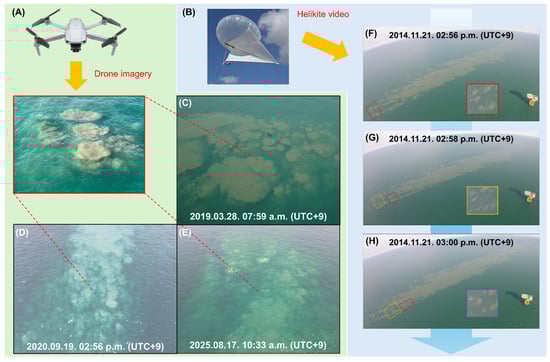
Figure 5.
(A) UAV platform. (B) Helikite platform. (C–E) Patchy structure of the Ieodo plume observed in UAV RGB imagery above the Ieodo summit. (F–H) Early-stage dynamics of the Ieodo plume observed in RGB imagery acquired using a GoPro camera mounted on a helikite.
However, patches of the Ieodo plume did not invariably reach the sea surface. An internal report (not published) by the Korea Institute of Ocean Science and Technology (KIOST) regarding the Ieodo plume states that during the summer, the plume fails to reach the surface layer and instead disperses within the bottom layer. Identifying the morphology of the Ieodo plume during summer using satellite observations is challenging because, during this period (June–September), the East China Sea often experiences increased cloudiness due to enhanced convection associated with higher sea-surface temperatures, the formation of a quasi-stationary front, and frequent tropical cyclones, resulting in a limited number of usable satellite scenes. In particular, for July and August, no images capturing the Ieodo plume were found in either the Sentinel-2 or GOCI-II datasets during the study period.
Low-altitude remote sensing is advantageous under such circumstances because it acquires data below the cloud level, is less sensitive to meteorological constraints than satellite imagery, and, owing to its high spatial resolution on the order of several tens of centimeters, can detect weak signals that are difficult to discern from satellites. Accordingly, hovering UAV observations were conducted in August 2025 to examine the behavior of the Ieodo plume during summer. UAV imagery confirmed that, even in summer, the Ieodo plume occurred and dispersed from the same source location (Figure 6A,C). The plume observed on this occasion appeared closer to bright green than the plumes observed at other times, exhibited a narrower initial width, and had smaller patch sizes. On this date, the Ieodo plume could not be identified in the GOCI-II data (Figure 6B,D). Thus, the Ieodo plume can be detected through drone-based observations, even when the satellite sensors do not clearly identify the plume.
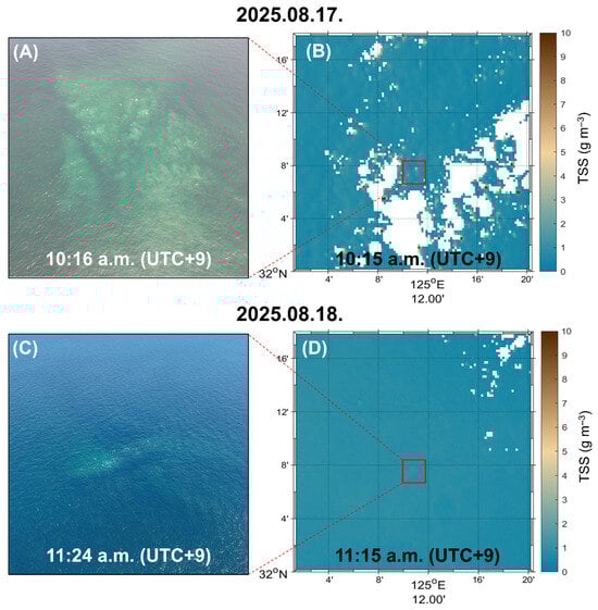
Figure 6.
(A,C) Summertime Ieodo plume occurrence observed by UAV-based observations. (B,D) Ieodo plume that is difficult to identify in contemporaneous GOCI-II TSS imagery.
Simultaneously, seawater samples were remotely collected at four sites over the Ieodo plume using a UAV deployed from the I-ORS, and the SPM concentrations were analyzed (Figure 7). The SPM concentration was calculated as shown in Equation (2), where w1 and w2 denote the weights of the filter paper before and after filtration, respectively, and V represents the volume of the filtered seawater.
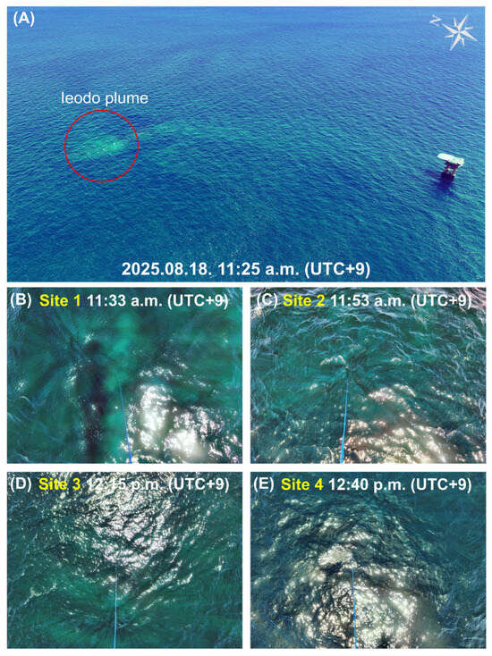
Figure 7.
(A) Morphology of the Ieodo plume captured by UAV-based imaging (green band contrast-adjusted RGB image). (B–E) Sampling locations for Ieodo plume seawater samples (green band contrast-adjusted RGB image). A water sampler, connected to the blue tether, was deployed from the UAV.
The analysis showed that SPM concentrations in seawater samples collected from multiple locations (Sites 1–4, Figure 7B–E) within the plume area ranged from 0.22 to 2.66 mg L−1 within the plume-occurrence area (Table 3). These values are remarkably low even within the concentration range generally classified as clear waters (<10 mg L−1) and are comparable to levels observed in very clean offshore environments [66,67]. Given that turbid water with a distinct color was clearly visible in the optical images, these findings suggest that the plume-associated sediments did not reach the sea surface during the study period. Meanwhile, SPM concentrations in seawater samples collected by basket sampling directly beneath the I-ORS immediately after UAV sampling—where no plume-related turbidity signal was detected—were even lower, at 0.12–0.16 mg L−1 (Table 3).
Table 3.
SPM concentrations in seawater samples retrieved from the Ieodo plume region on 18 August 2025.
3.3. Mechanism of the Ieodo Plume
Through integrated observations using satellite and UAV imagery, it was revealed that the Ieodo plume originates from the summit of the Ieodo Seamount, and its initial form is an aggregated patch of fine-grained sediments. In general, for sediments that are denser than seawater to be resuspended and reach the surface, substantial forcing is required. In the case of the Ieodo plume, this forcing is derived from strong current velocities. In the East China Sea, where tidal currents dominate, the bathymetry of the Ieodo Seamount generates faster flows than those in the surrounding area around the summit. This process can be interpreted in terms of the Bernoulli principle (Figure 8A,B). The acceleration of tidal currents, which have been flowing over the flat seafloor as they pass over the summit along the seamount slope, follows the same principle by which a fluid accelerates when it traverses a conduit with a reduced cross-sectional area.
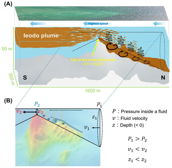
Figure 8.
(A) Schematic illustration of the Ieodo plume generation mechanism under southward tidal flow conditions. (B) Conceptual illustration of the Ieodo plume generation in terms of the Bernoulli principle.
While the Bernoulli equation assumes a steady flow of an inviscid, incompressible fluid, the real ocean exhibits unsteady currents, turbulent and viscous flow, and density differences caused by stratification. Nevertheless, when temporal variations in the flow are relatively slow and viscous effects can be regarded as small, it is possible to apply the physical concept embodied in the Bernoulli equation locally under quasi-steady conditions, namely, the conversion among pressure, kinetic energy, and potential energy. The Ieodo region is dominated by tidal currents, and the Reynolds number is far greater than one; accordingly, viscous effects may be neglected. Assuming hydrostatic pressure, the quasi-steady Bernoulli equation, including the time-derivative term of the velocity potential, is defined as Equation (3).
Near the point where the Ieodo Seamount topography begins, denotes the internal pressure of the fluid, is the flow speed, is the water depth, and is the velocity potential. , , , and denote, respectively, the internal pressure, flow speed, water depth, and velocity potential in the vicinity of the Ieodo summit.
Meanwhile, because the Ieodo plume exhibits a distinct streamlined flow depending on the tidal-current direction and the temporal change in the tidal current is gradual, one may take , which permits approximation to the steady Bernoulli equation by eliminating the time-derivative term of the velocity potential, as in Equation (4).
As illustrated in Figure 8B, let us assume a southward tidal-current flow along the northern slope of the Ieodo Seamount. As the flow moves upslope toward the summit, the seamount topography reduces the effective cross-sectional width between the sea surface and the seabed, thereby increasing , whereas the negative depth also increases (i.e., becomes less negative). Accordingly, and ; through conservation of energy, the internal fluid pressure near the summit must decrease relative to that upstream, such that . This pressure reduction can act as a mechanism that draws suspended sediments upward toward the sea surface.
To demonstrate the Bernoulli-related increase in flow speed in the vicinity of the Ieodo summit, currents in the plume generation area were estimated by tracking the motion of plume particles on 42 sets of orthorectified sequential images of the Ieodo plume, which were acquired during UAV hovering observations, using LSPIV in MATLAB (Figure 9A–D). The mean u- and v-component velocities, representing the plume-particle displacement, were extracted at 187 points along a straight transect following the center of the plume.
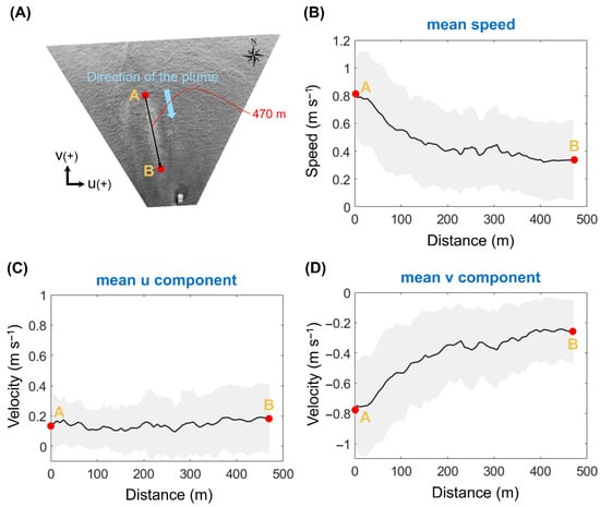
Figure 9.
Results of LSPIV analyses from a set of 42 geometrically corrected, sequential UAV images capturing the Ieodo plume. (A) Geometrically corrected UAV image. (B) Mean speed of the combined u–v vector. (C) Mean u-component velocity. (D) Mean v-component velocity. The gray-shaded area represents the standard deviation.
The mean speed of the plume decreased progressively from 0.81 ± 0.30 m s−1 at point A near the summit to 0.34 ± 0.29 m s−1 at point B, located 470 m away from point A (Figure 9B). The mean u-component velocity, which partly describes diffusion in the direction perpendicular to the plume’s center, increased slightly from 0.13 ± 0.19 m s−1 at point A to 0.18 ± 0.23 m s−1 at point B (Figure 9C). The mean u-component always remained greater than zero because, in the orthorectified imagery, the centerline of the plume migrated consistently in the direction of increasing u. On the other hand, the mean v-component velocity, which indicates the primary component of plume advection, showed a similar pattern to that of the mean total speed: it was highest at point A, 0.79 ± 0.29 m s−1, and gradually decreased to 0.26 ± 0.21 m s−1 at point B (Figure 9D). Therefore, the velocity variations estimated by LSPIV in the plume area provide evidence of localized current acceleration near the summit, owing to Bernoulli’s principle.
4. Discussion
4.1. Detection of the Ieodo Plume in Satellite Imagery
Sentinel-2 and GOCI-II satellite data were used to detect and analyze the morphology of the Ieodo plume in this study. Although the northern East China Sea, the study area, is classified as Case 2 waters strongly influenced by suspended constituents, the Ieodo plume is confined to the vicinity of the I-ORS and exhibits distinctive band- or ring-shaped structures; thus, it can be readily identified in satellite imagery. Here, we selected well-developed Ieodo plume events that disperse with clear boundaries distinguishable from the surrounding seawater by jointly considering these morphological characteristics, the geolocation of the I-ORS, and the TSS products. Based on these standards, the spatial and morphological characteristics of the plume and its hourly behavior were analyzed.
However, this approach may fail to capture ‘weak’ plumes, such as small-scale plumes with blurred boundaries during dispersion or those at an early developmental stage. In such cases, Ieodo plumes may exhibit TSS values below 10 g m−3; consequently, their occurrence may be difficult to detect using a TSS threshold alone. In addition, the contributions of optically active constituents other than sediments were not explicitly separated or accounted for in this analysis. The Ieodo plume may also be identified using other GOCI-II products, such as chlorophyll a (Chl-a) and colored dissolved organic matter (CDOM) (Figure 10). This suggests that the optical signal of the plume may also be influenced by other materials. Thus, thresholding based on multiple parameters may provide improved discrimination between the plume and surrounding waters.
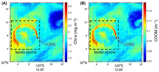
Figure 10.
The Ieodo plume identified in other GOCI-II products on October 31, 2023: (A) Chl-a. (B) CDOM.
Therefore, to more comprehensively assess the frequency of occurrence and the spatial extent of the Ieodo plume, future work would require quantitative approaches that can robustly detect and discriminate plume signals, including weak or developing cases. Such efforts may be complemented by applying spectral information and algorithm-based methods for plume delineation and classification (e.g., machine learning classification), as well as by conducting field investigations to characterize the suspended constituents of the Ieodo plume.
4.2. Patchy Structure of the Ieodo Plume
In this study, we explain the fundamental generation mechanism of the Ieodo plume based on the Bernoulli effect induced by tidal currents flowing over the local seabed topography around Ieodo. However, the question of why the Ieodo plume initially emerges as a localized, patch-like feature remains open to further discussion. A substantial body of previous work, including Rood and Hickin, Kostaschuk, Smith et al., Thorpe, and Talke et al. [68,69,70,71,72], has shown that strong tidal currents flowing over seabed topography can generate intermittent bursting events such as bottom “boils,” during which resuspended fine-grained sediments may be transported vertically throughout the water column. In particular, Kwoll [73] explains the generation mechanism of “turbidity clouds,” which are similar in appearance to the Ieodo plume caused by tidal currents exceeding a critical velocity and coherent flow structures. Thus, the mechanisms by which turbulent flows, induced by the interaction between seabed topography and tides, capture resuspended sediments and transport them to the sea surface have been reported across a range of estuarine, shallow-water, and continental-shelf environments.
As discussed previously, the Ieodo region has sufficient conditions for the operation of such mechanisms. The Ieodo Seamount, where the Ieodo plume occurs, is an elevated bathymetric feature that protrudes from a gently sloping continental shelf. In addition, the dominant semidiurnal tidal flow provides favorable conditions for strong near-bed shear, and intermittent turbulence is induced by topographic rises distributed along the seamount slope. This turbulence can drive the vertical transport of fluid from the bottom layer toward the sea surface, thereby enabling resuspended sediments to reach the surface in the form of multiple localized patches. Therefore, it is reasonable to interpret that the initial generation of the Ieodo plume is driven by a decrease in internal fluid pressure according to Bernoulli’s principle for a macro scale and by the vertical transport induced by turbulent flow resulting from the interaction between tidal currents and seabed topography on a local scale.
To quantitatively test this hypothesis, additional analyses are required, including field-based measurements that utilize ADCPs, turbidimeters, and microstructure profilers. Furthermore, three-dimensional numerical modeling is necessary, which incorporates, at a high spatial resolution, the topography and physical forcing around the Ieodo Seamount, along with sediment distributions. If such multifaceted verification can elucidate the turbulent structures and resuspension processes that deliver the Ieodo plume to the sea surface in patch form, the Ieodo plume phenomenon can be more clearly understood within the conceptual framework of interactions among topography, tides, turbulence, and sediments.
4.3. Summer Stratification in the Ieodo Region and Subsurface Dispersion of the Ieodo Plume
As presented in Result 2, both the UAV observations and in situ seawater sampling results indicated that the suspended sediments in the Ieodo plume did not reach the sea surface in August 2025. This finding suggests that seawater stratification was strengthened in the Ieodo region during this period. In summer, low-density surface waters may develop due to intensified solar radiation and associated surface warming, together with freshwater inputs from precipitation.
Quality-controlled, depth-resolved temperature data from the CTD sensor at the I-ORS for August 2025 show an apparent temperature contrast between the surface and bottom layers throughout the month (Figure 11A). Despite short-term variability, the trends in surface and deep-water temperatures persisted, indicating that the thermal structure of the water column was maintained. The concurrent meteorological records provide additional context for interpreting the atmospheric conditions during the same period (Figure 10B). Insolation remained high on most days, reaching peak values of ~1000 W/m2, except for the rainfall event on 11 August, which represents strong daytime surface heating. Taken together, these thermal and meteorological data support the interpretation that there was a clear ocean stratification in the Ieodo region during the UAV observation period in 2025.
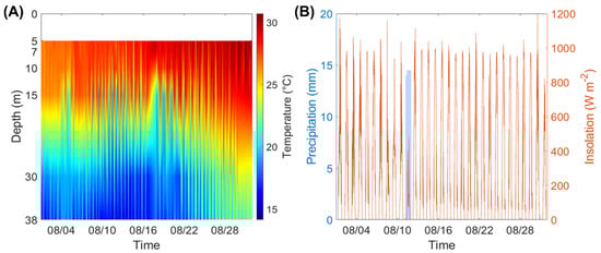
Figure 11.
(A) 10 min interval, quality-controlled CTD temperature profiles obtained from the I-ORS in August 2025 at discrete depths of 5, 7, 10, 15, 30, and 38 m; missing values were linearly interpolated. (B) Precipitation (left axis; blue shading) and insolation (right axis; orange line) over the same period.
In addition, in the East China Sea, surface freshening associated with Changjiang diluted water (CDW)—a low-salinity, low-density surface water mass originating from the Changjiang (Yangtze) River in China—has been widely reported, particularly from June to September. CDW is commonly defined as water with a surface salinity below approximately 31 psu and is known to extend to a maximum depth of 20 m in the East China Sea during summer [74,75]. Numerous studies have further demonstrated that, in summer, particularly in July and August, the CDW can influence waters near the Korean Peninsula [76,77,78,79].
Owing to these factors, the warm, low-salinity surface water mass that forms in the Ieodo region during summer strengthens the vertical density gradient, thereby suppressing the development of the turbulence required for Ieodo plume formation. Under such conditions, the resuspended sediments may fail to become buoyant and reach the surface, thus remaining and dispersing at depths below the low-density layer.
Meanwhile, considering that the Ieodo plume forms near the summit along the Ieodo Seamount topography, when the plume becomes sufficiently developed for visual observation, its dispersion depth is expected to be shallower than the summit depth of 4.6 m, even if it does not reach the surface. However, because the in situ CTD at the I-ORS measures temperature and salinity only at depths of 5 m and deeper, its ability to resolve the specific depth range of the low-density layer that inhibits the plume from reaching the surface is limited. Accordingly, additional near-surface data from further surveys are required to determine the precise depth at which the Ieodo plume disperses below the sea surface.
4.4. The LSPIV Algorithm and Direct Georeferencing
In this study, the planar flow field of the plume was estimated from UAV imagery using the LSPIV algorithm. This is one of the most viable alternatives for deriving flow velocities in environments where the operation of in situ current-measurement instruments is constrained. The flow field was effectively derived from the LSPIV because the Ieodo plume exhibited a distinct contrast with ambient waters, and fine sediment constituents in the plume served as passive tracers of the flow.
However, the LSPIV approach is basically optimized for tracking particles floating on the sea surface. Because the imagery analyzed in this study addresses the special circumstances in which the plume disperses below the sea surface, it was necessary to remove as many surface signals as possible, such as waves and sun glint. Given that the plume advection direction identified in the imagery was clearly opposite to the wave propagation direction, we removed all signals whose v-direction velocities were oriented opposite to the plume. In addition, we delineated only the region in which the plume was identifiable and removed strong signals exceeding the maximum surface current speeds previously reported for the Ieodo region, thereby minimizing the possibility of tracking features other than plume particles.
In addition, the direct georeferencing technique for the orthorectification of drone imagery before LSPIV analysis requires further refinement. Unlike land-based remote sensing, in which GCPs are used to ensure geometric precision, these methods cannot be readily applied to dynamic oceanic settings. Therefore, orthorectification in marine remote sensing is highly dependent on the onboard GPS and IMU sensors of the platform. In particular, when using a UAV, minor distortions can occur during posture adjustments required to maintain position. These effects are particularly evident under windy and gusty conditions. Although this study assumed a stationary drone position during the hovering phase for preprocessing, more rigorous orthorectification approaches are required for future applications.
4.5. Jet–Plume Theory
In this study, we analyzed the behavior and dispersion of the Ieodo plume using remote sensing approaches based on satellite and UAV observations. However, as noted in the Introduction, there are multiple approaches to investigate the dispersion of suspended sediment plumes in the ocean beyond remote sensing. In particular, theoretical and numerical model-based approaches are also applicable to the Ieodo plume because its forcing structure is relatively simpler than that observed in coastal settings. Specifically, with appropriate initial and boundary conditions, a scaling analysis based on the jet–plume theory can be used to quantitatively assess when an initially momentum-dominated Ieodo plume transitions to a flow that is more strongly influenced by the ambient background field.
The jet–plume theory is a classical mixing framework developed to describe turbulent flow originating from a localized source that transitions from a momentum jet to a buoyant plume. Morton, Taylor, and Turner [19] treated turbulent flows generated by point- or line-shaped buoyancy sources as cross-sectionally integrated structures and formulated integral conservation equations for volume, momentum, and buoyancy fluxes across the plume section. Moreover, by assuming that turbulent entrainment at the plume edge is proportional to the characteristic centerline velocity, they simplified an otherwise complex turbulence problem and quantitatively described how the plume width, velocity, and related properties evolve as the plume develops, thereby providing the foundation for classical plume theory. Fischer [20] subsequently applied this framework to real environmental problems, such as coastal and estuarine settings, and systematized the concept of a buoyant jet, in which the flow is initially momentum-dominated; however, beyond a specific time and distance, it becomes buoyancy-dominated. In doing so, Fischer argued that jets and plumes are not independent categories but rather represent segments within a continuous flow, distinguished by the dominant regime. In this context, by additionally accounting for factors such as stratification and background currents in marine environments, various length scales and non-dimensional parameters were introduced to provide quantitative criteria for determining the portion of the flow for which a jet approximation is valid and confirming beyond which portion of the plume approximation becomes appropriate.
Because jet–plume theory presupposes a flow initiated from a localized point or line source, applying it to naturally occurring resuspended sediment plumes may appear inappropriate at first glance. However, as discussed above, the Ieodo plume repeatedly originates from a fixed location; thus, from a macroscopic perspective, the summit region of Ieodo may be idealized as a single source whose initial discharge direction follows the tidal current. This allows for the application of this approach to the Ieodo plume problem. That is, if the Ieodo plume is regarded as a buoyant jet that, near the source, exhibits a jet-like regime in which the orientation of plume patches is closely aligned with the tidal-current vector, and then transitions beyond a certain distance to a plume-like regime dominated by buoyancy and the background field. This process can be interpreted within the same classical theoretical framework.
From this perspective, the Ieodo plume may be viewed as an observational case wherein regime transitions of a buoyant jet, as discussed in classical jet–plume theory, can be examined in the real ocean. The length scales and nondimensional numbers required to diagnose each regime could be evaluated more quantitatively in future work if the essential initial conditions and background constraints, such as ambient currents and stratification, are obtained from field observations. Furthermore, interpreting the Ieodo plume through jet–plume theory may provide a useful theoretical basis for predicting the behavior and impacts of flows with similar dynamical characteristics, including estuarine plumes with fixed source locations and suspended sediment plumes generated by anthropogenic activities such as dredging and mining.
5. Conclusions
Based on integrated satellite and low-altitude remote sensing observations, we examined the Ieodo plume’s dispersal and its morphological and dynamical characteristics. The main conclusions are as follows:
- Satellite observations indicated that the Ieodo plume repeatedly originates from a point on the summit of the Ieodo Seamount, located near the I-ORS. Exhibiting an initial width of approximately 0.5 km, it develops into a band-shaped structure that curves counterclockwise and disperses over a spatial extent of 11.4 ± 3.2 km in the east–west direction and 14.3 ± 4.1 km in the north–south direction. The initial development of the Ieodo plume was controlled by tidal currents, with the highest TSS occurring when the southward current component was strongest during the day. Following its formation, the band or ring structure of the plume underwent a counterclockwise curvature during its clockwise rotation along the tidal ellipse, and the TSS of the plume decreased with time.
- The UAV observations revealed that the Ieodo plume was initially composed of circular sediment aggregates during its initial stage. After reaching the surface, these patches began to flow along the surface currents and merged with the previously formed sediment band structure observed in the satellite imagery. In addition, SPM analyses of surface seawater samples remotely collected by UAV at the time of plume occurrence indicate that during summer, when stratification is pronounced, the Ieodo plume does not fully rise to the sea surface; instead, it disperses below the surface, making it difficult to identify using satellite observations.
- Velocity estimation via LSPIV analysis of georeferenced sequential UAV imagery indicated that the plume speed was highest near the origin and gradually decreased as it dispersed horizontally. In accordance with the interactions between tidal forcing and the topography of the Ieodo Seamount, this behavior can be explained by the Bernoulli principle, which states that flow accelerates as the flow passage narrows. Similarly, the mechanism by which sediments composing the Ieodo plume are lofted toward the sea surface can be interpreted as arising from a reduction in internal fluid pressure, which is required to compensate for increases in flow speed under the conservation of total energy.
These findings demonstrate the utility of integrated remote sensing for investigating submesoscale marine physical phenomena and provide a basis for assessing and predicting the dispersion and impacts of suspended sediment plumes in the ocean, which exhibit dynamical mechanisms and spatial scales comparable to those of the Ieodo plume.
Author Contributions
Conceptualization, S.H. and Y.-H.J.; methodology, S.H., W.L. and Y.-H.J.; software, S.H., S.-Y.K. and J.-S.L.; validation, S.H.; formal analysis, S.H.; investigation, S.H., S.-Y.K., W.L. and S.-C.L.; resources, S.H., S.-C.L. and J.-Y.J.; data curation, S.H.; writing—original draft preparation, S.H.; writing—review and editing, S.H. and Y.-H.J.; visualization, S.H.; supervision, Y.-H.J.; project administration, Y.-H.J.; funding acquisition, Y.-H.J. All authors have read and agreed to the published version of the manuscript.
Funding
This research was supported by the Korea Institute of Marine Science & Technology Promotion (KIMST) project (RS-2021-KS211502, Establishment of the Ocean Research Station in the Jurisdiction Zone and Convergence Research).
Data Availability Statement
Data are contained within the article.
Acknowledgments
The authors thank the Korea Institute of Ocean Science and Technology, Busan, South Korea, for providing past observational data.
Conflicts of Interest
The authors declare no conflicts of interest.
References
- Zhang, J. Heavy Metal Compositions of Suspended Sediments in the Changjiang (Yangtze River) Estuary: Significance of Riverine Transport to the Ocean. Cont. Shelf Res. 1999, 19, 1521–1543. [Google Scholar] [CrossRef]
- Turner, A.; Millward, G.E. Suspended Particles: Their Role in Estuarine Biogeochemical Cycles. Estuar. Coast. Shelf Sci. 2002, 55, 857–883. [Google Scholar] [CrossRef]
- Schoellhamer, D.H.; Mumley, T.E.; Leatherbarrow, J.E. Suspended Sediment and Sediment-Associated Contaminants in San Francisco Bay. Environ. Res. 2007, 105, 119–131. [Google Scholar] [CrossRef]
- Wilber, D.H.; Clarke, D.G. Biological Effects of Suspended Sediments: A Review of Suspended Sediment Impacts on Fish and Shellfish with Relation to Dredging Activities in Estuaries. N. Am. J. Fish. Manag. 2001, 21, 855–875. [Google Scholar] [CrossRef]
- Erftemeijer, P.L.A.; Riegl, B.; Hoeksema, B.W.; Todd, P.A. Environmental Impacts of Dredging and Other Sediment Disturbances on Corals: A Review. Mar. Pollut. Bull. 2012, 64, 1737–1765. [Google Scholar] [CrossRef] [PubMed]
- Zhang, H.; Zhao, L.; Sun, Y.; Wang, J.; Wei, H. Contribution of Sediment Oxygen Demand to Hypoxia Development off the Changjiang Estuary. Estuar. Coast. Shelf Sci. 2017, 192, 149–157. [Google Scholar] [CrossRef]
- Carreiro-Silva, M.; Martins, I.; Riou, V.; Raimundo, J.; Caetano, M.; Bettencourt, R.; Rakka, M.; Cerqueira, T.; Godinho, A.; Morato, T.; et al. Mechanical and Toxicological Effects of Deep-Sea Mining Sediment Plumes on a Habitat-Forming Cold-Water Octocoral. Front. Mar. Sci. 2022, 9, 915650. [Google Scholar] [CrossRef]
- Bai, M.; Dong, F.; Jia, Y.; Qi, B.; Yu, S.; Peng, S.; Liang, B.; Li, L.; Yu, L.; Zhang, X.; et al. Impact of Sediment Plume on Benthic Microbial Community in Deep-Sea Mining. Water 2025, 17, 3013. [Google Scholar] [CrossRef]
- Shields, A. Application of Similarity Principles and Turbulence Research to Bed-Load Movement; California Institute of Technology: Pasadena, CA, USA, 1936. [Google Scholar]
- Luo, Z.; Zhu, J.; Wu, H.; Li, X. Dynamics of the Sediment Plume over the Yangtze Bank in the Yellow and East China Seas. J. Geophys. Res. Oceans. 2017, 122, 10073–10090. [Google Scholar] [CrossRef]
- Yuan, Y.; Wei, H.; Zhao, L.; Cao, Y. Implications of Intermittent Turbulent Bursts for Sediment Resuspension in a Coastal Bottom Boundary Layer: A Field Study in the Western Yellow Sea, China. Mar. Geol. 2009, 263, 87–96. [Google Scholar] [CrossRef]
- Salim, S.; Pattiaratchi, C.; Tinoco, R.; Coco, G.; Hetzel, Y.; Wijeratne, S.; Jayaratne, R. The Influence of Turbulent Bursting on Sediment Resuspension under Unidirectional Currents. Earth Surf. Dynam. 2017, 5, 399–415. [Google Scholar] [CrossRef]
- Geyer, W.R.; Hill, P.S.; Kineke, G.C. The Transport, Transformation and Dispersal of Sediment by Buoyant Coastal Flows. Cont. Shelf Res. 2004, 24, 927–949. [Google Scholar] [CrossRef]
- Marques, W.C.; Fernandes, E.H.L.; Moraes, B.C.; Möller, O.O.; Malcherek, A. Dynamics of the Patos Lagoon Coastal Plume and Its Contribution to the Deposition Pattern of the Southern Brazilian Inner Shelf. J. Geophys. Res. Oceans. 2010, 115, C10045. [Google Scholar] [CrossRef]
- Brando, V.E.; Braga, F.; Zaggia, L.; Giardino, C.; Bresciani, M.; Matta, E.; Bellafiore, D.; Ferrarin, C.; Maicu, F.; Benetazzo, A.; et al. High-Resolution Satellite Turbidity and Sea Surface Temperature Observations of River Plume Interactions during a Significant Flood Event. Ocean Sci. 2015, 11, 909–920. [Google Scholar] [CrossRef]
- Devlin, M.J.; Petus, C.; Da Silva, E.; Tracey, D.; Wolff, N.H.; Waterhouse, J.; Brodie, J. Water Quality and River Plume Monitoring in the Great Barrier Reef: An Overview of Methods Based on Ocean Colour Satellite Data. Remote Sens. 2015, 7, 12909–12941. [Google Scholar] [CrossRef]
- Spearman, J. A Review of the Physical Impacts of Sediment Dispersion from Aggregate Dredging. Mar. Pollut. Bull. 2015, 94, 260–277. [Google Scholar] [CrossRef]
- Gillard, B.; Purkiani, K.; Chatzievangelou, D.; Vink, A.; Iversen, M.H.; Thomsen, L. Physical and Hydrodynamic Properties of Deep Sea Mining-Generated, Abyssal Sediment Plumes in the Clarion Clipperton Fracture Zone (Eastern-Central Pacific). Elem. Sci. Anth. 2019, 7, 5. [Google Scholar] [CrossRef]
- Morton, B.R.; Taylor, G.; Turner, J.S. Turbulent Gravitational Convection from Maintained and Instantaneous Sources. Proc. R. Soc. Lond. Ser. A 1956, 234, 1–23. [Google Scholar] [CrossRef]
- Fischer, H.; List, E.; Koh, R.; Imberger, J.; Brooks, N. Mixing in Inland and Coastal Waters; Academic Press: London, UK, 1979. [Google Scholar] [CrossRef]
- Woods, A.W. Turbulent Plumes in Nature. Annu. Rev. Fluid Mech. 2010, 42, 391–412. [Google Scholar] [CrossRef]
- Gerritsen, H.; Vos, R.J.; van der Kaaij, T.; Lane, A.; Boon, J.G. Suspended Sediment Modelling in a Shelf Sea (North Sea). Coast. Eng. 2000, 41, 317–352. [Google Scholar] [CrossRef]
- Bass, S.J.; Aldridge, J.N.; McCave, I.N.; Vincent, C.E. Phase Relationships between Fine Sediment Suspensions and Tidal Currents in Coastal Seas. J. Geophys. Res. Oceans. 2002, 107, 10-1–10-14. [Google Scholar] [CrossRef]
- Purkiani, K.; Gillard, B.; Paul, A.; Haeckel, M.; Haalboom, S.; Greinert, J.; de Stigter, H.; Hollstein, M.; Baeye, M.; Vink, A.; et al. Numerical Simulation of Deep-Sea Sediment Transport Induced by a Dredge Experiment in the Northeastern Pacific Ocean. Front. Mar. Sci. 2021, 8, 719463. [Google Scholar] [CrossRef]
- Nazirova, K.; Alferyeva, Y.; Lavrova, O.; Shur, Y.; Soloviev, D.; Bocharova, T.; Strochkov, A. Comparison of In Situ and Remote-Sensing Methods to Determine Turbidity and Concentration of Suspended Matter in the Estuary Zone of the Mzymta River, Black Sea. Remote Sens. 2021, 13, 143. [Google Scholar] [CrossRef]
- Uehara, K.; Saito, Y. Late Quaternary Evolution of the Yellow/East China Sea Tidal Regime and Its Impacts on Sediments Dispersal and Seafloor Morphology. Sediment. Geol. 2003, 162, 25–38. [Google Scholar] [CrossRef]
- Nechad, B.; Ruddick, K.G.; Park, Y. Calibration and Validation of a Generic Multisensor Algorithm for Mapping of Total Suspended Matter in Turbid Waters. Remote Sens. Environ. 2010, 114, 854–866. [Google Scholar] [CrossRef]
- Tavora, J.; Gonçalves, G.A.; Fernandes, E.H.; Salama, M.S.; van der Wal, D. Detecting Turbid Plumes from Satellite Remote Sensing: State-of-Art Thresholds and the Novel PLUMES Algorithm. Front. Mar. Sci. 2023, 10, 1215327. [Google Scholar] [CrossRef]
- Liu, Z.; Jiao, S.; Liu, X.; Lv, X. Two-Dimensional Numerical Simulation of Tide and Tidal Current of Eight Major Tidal Constituents in the Bohai, Yellow, and East China Seas. Remote Sens. 2023, 15, 3735. [Google Scholar] [CrossRef]
- Jeong, T.-B.; Kim, Y.S.; Cha, H.; Jeong, K.-Y.; Jeong, J.-Y.; Lee, J.-H. Application of Quality-Controlled Sea Level Height Observation at the Central East China Sea: Assessment of Sea Level Rise. Ocean Sci. 2025, 21, 2085–2099. [Google Scholar] [CrossRef]
- Van Lancker, V.; Baeye, M. Wave Glider Monitoring of Sediment Transport and Dredge Plumes in a Shallow Marine Sandbank Environment. PLoS ONE 2015, 10, e0128948. [Google Scholar] [CrossRef]
- Spearman, J.; Taylor, J.; Crossouard, N.; Cooper, A.; Turnbull, M.; Manning, A.; Lee, M.; Murton, B. Measurement and Modelling of Deep Sea Sediment Plumes and Implications for Deep Sea Mining. Sci. Rep. 2020, 10, 5075. [Google Scholar] [CrossRef]
- Haalboom, S.; Schoening, T.; Urban, P.; Gazis, I.-Z.; de Stigter, H.; Gillard, B.; Baeye, M.; Hollstein, M.; Purkiani, K.; Reichart, G.-J.; et al. Monitoring of Anthropogenic Sediment Plumes in the Clarion-Clipperton Zone, NE Equatorial Pacific Ocean. Front. Mar. Sci. 2022, 9, 882155. [Google Scholar] [CrossRef]
- Gazis, I.-Z.; de Stigter, H.; Mohrmann, J.; Heger, K.; Diaz, M.; Gillard, B.; Baeye, M.; Veloso-Alarcón, M.E.; Purkiani, K.; Haeckel, M.; et al. Monitoring Benthic Plumes, Sediment Redeposition and Seafloor Imprints Caused by Deep-Sea Polymetallic Nodule Mining. Nat. Commun. 2025, 16, 1229. [Google Scholar] [CrossRef] [PubMed]
- Chang, T.S.; Jeong, J.O.; Lee, E.; Byun, D.-S.; Lee, H.-Y.; Son, C.S. Distribution Patterns and Provenance of Surficial Sediments from Ieodo and Adjacent Sea. J. Korean Earth Sci. Soc. 2020, 41, 588–598. [Google Scholar] [CrossRef]
- Jo, Y.-H.; Sha, J.; Kwon, J.-I.; Jun, K.-C.; Park, J. Mapping Bathymetry Based on Waterlines Observed from Low Altitude Helikite Remote Sensing Platform. Acta Oceanol. Sin. 2015, 34, 110–116. [Google Scholar] [CrossRef]
- Jo, Y.-H.; Bi, H.; Lee, J.-S. Potential Applications of Low Altitude Remote Sensing for Monitoring Jellyfish. Korean J. Remote Sens. 2017, 33, 15–24. [Google Scholar] [CrossRef]
- Mobley, C.D. Estimation of the Remote-Sensing Reflectance from above-Surface Measurements. Appl. Opt. 1999, 38, 7442–7455. [Google Scholar] [CrossRef]
- Nezlin, N.P.; Weisberg, S.B.; Diehl, D.W. Relative Availability of Satellite Imagery and Ship-Based Sampling for Assessment of Stormwater Runoff Plumes in Coastal Southern California. Estuar. Coast. Shelf Sci. 2007, 71, 250–258. [Google Scholar] [CrossRef]
- Fettweis, M.P.; Nechad, B. Evaluation of In Situ and Remote Sensing Sampling Methods for SPM Concentrations, Belgian Continental Shelf (Southern North Sea). Ocean Dyn. 2011, 61, 157–171. [Google Scholar] [CrossRef]
- Lee, J.-S.; Baek, J.-Y.; Shin, J.; Kim, J.-S.; Jo, Y.-H. Suspended Sediment Concentration Estimation along Turbid Water Outflow Using a Multispectral Camera on an Unmanned Aerial Vehicle. Remote Sens. 2023, 15, 5540. [Google Scholar] [CrossRef]
- Lally, H.T.; O’Connor, I.; Jensen, O.P.; Graham, C.T. Can Drones Be Used to Conduct Water Sampling in Aquatic Environments? A Review. Sci. Total Environ. 2019, 670, 569–575. [Google Scholar] [CrossRef]
- Adrian, R.J. Particle-Imaging Techniques for Experimental Fluid Mechanics. Annu. Rev. Fluid Mech. 1991, 23, 261–304. [Google Scholar] [CrossRef]
- Raffel, M.; Willert, C.E.; Scarano, F.; Kähler, C.J.; Wereley, S.T.; Kompenhans, J. Particle Image Velocimetry: A Practical Guide, 3rd ed.; Springer: Cham, Switzerland, 2018. [Google Scholar] [CrossRef]
- Muste, M.; Fujita, I.; Hauet, A. Large-Scale Particle Image Velocimetry for Measurements in Riverine Environments. Water Resour. Res. 2008, 44, W00D19. [Google Scholar] [CrossRef]
- Tauro, F.; Petroselli, A.; Grimaldi, S. Optical Sensing for Stream Flow Observations: A Review. J. Agric. Eng. 2018, 49, 199–206. [Google Scholar] [CrossRef]
- Perks, M.T.; Fortunato Dal Sasso, S.; Hauet, A.; Jamieson, E.; Le Coz, J.; Pearce, S.; Peña-Haro, S.; Pizarro, A.; Strelnikova, D.; Tauro, F.; et al. Towards Harmonisation of Image Velocimetry Techniques for River Surface Velocity Observations. Earth Syst. Sci. Data 2020, 12, 1545–1559. [Google Scholar] [CrossRef]
- Tauro, F.; Pagano, C.; Phamduy, P.; Grimaldi, S.; Porfiri, M. Large-Scale Particle Image Velocimetry from an Unmanned Aerial Vehicle. IEEE/ASME Trans. Mechatron. 2015, 20, 3269–3275. [Google Scholar] [CrossRef]
- Lewis, Q.W.; Lindroth, E.M.; Rhoads, B.L. Integrating Unmanned Aerial Systems and LSPIV for Rapid, Cost-Effective Stream Gauging. J. Hydrol. 2018, 560, 230–246. [Google Scholar] [CrossRef]
- Wang, J.; Ge, Y.; Heuvelink, G.B.M.; Zhou, C.; Brus, D. Effect of the Sampling Design of Ground Control Points on the Geometric Correction of Remotely Sensed Imagery. Int. J. Appl. Earth Obs. Geoinf. 2012, 18, 91–100. [Google Scholar] [CrossRef]
- Helgesen, H.H.; Leira, F.S.; Bryne, T.H.; Albrektsen, S.M.; Johansen, T.A. Real-Time Georeferencing of Thermal Images Using Small Fixed-Wing UAVs in Maritime Environments. ISPRS J. Photogramm. Remote Sens. 2019, 154, 84–97. [Google Scholar] [CrossRef]
- Zhang, K.; Okazawa, H.; Hayashi, K.; Hayashi, T.; Fiwa, L.; Maskey, S. Optimization of Ground Control Point Distribution for Unmanned Aerial Vehicle Photogrammetry for Inaccessible Fields. Sustainability 2022, 14, 9505. [Google Scholar] [CrossRef]
- Elaaraj, A.; Lhachmi, A.; Tabyaoui, H.; Alitane, A.; Varasano, A.; Hitouri, S.; El Yousfi, Y.; Mohajane, M.; Essahlaoui, N.; Gueddari, H.; et al. Remote Sensing Data for Geological Mapping in the Saka Region in Northeast Morocco: An Integrated Approach. Sustainability 2022, 14, 15349. [Google Scholar] [CrossRef]
- Özcihan, B.; Özlü, L.D.; Karakap, M.İ.; Sürmeli̇, H.; Alganci, U.; Sertel, E. A Comprehensive Analysis of Different Geometric Correction Methods for the Pleiades-1A and Spot-6 Satellite Images. Int. J. Eng. Geosci. 2023, 8, 146–153. [Google Scholar] [CrossRef]
- Román, A.; Heredia, S.; Windle, A.E.; Tovar-Sánchez, A.; Navarro, G. Enhancing Georeferencing and Mosaicking Techniques over Water Surfaces with High-Resolution Unmanned Aerial Vehicle (UAV) Imagery. Remote Sens. 2024, 16, 290. [Google Scholar] [CrossRef]
- Watts, J.; Holding, T.; Anderson, K.; Bell, T.G.; Chapron, B.; Donlon, C.; Collard, F.; Wood, N.; Walker, D.; DeBell, L.; et al. Georectifying Drone Image Data over Water Surfaces without Fixed Ground Control: Methodology, Uncertainty Assessment and Application over an Estuarine Environment. Estuar. Coast. Shelf Sci. 2024, 305, 108853. [Google Scholar] [CrossRef]
- Kim, S.-Y.; Lee, J.-S.; Jeong, Y.; Jo, Y.-H. Decomposition of Submesoscale Ocean Wave and Current Derived from UAV-Based Observation. Remote Sens. 2024, 16, 2275. [Google Scholar] [CrossRef]
- Saldías, G.S.; Sobarzo, M.; Largier, J.; Moffat, C.; Letelier, R. Seasonal Variability of Turbid River Plumes off Central Chile Based on High-Resolution MODIS Imagery. Remote Sens. Environ. 2012, 123, 220–233. [Google Scholar] [CrossRef]
- Petus, C.; Marieu, V.; Novoa, S.; Chust, G.; Bruneau, N.; Froidefond, J.-M. Monitoring Spatio-Temporal Variability of the Adour River Turbid Plume (Bay of Biscay, France) with MODIS 250-m Imagery. Cont. Shelf Res. 2014, 74, 35–49. [Google Scholar] [CrossRef]
- Mazzini, P.L.F.; Pianca, C.; Pareja-Roman, L.F.; Cole, K.L.; Walter, R.K.; Castelao, R.M.; Hunter, E.J.; Chant, R.J. Spatio-Temporal Variability of San Francisco Bay Plume from Space. Front. Mar. Sci. 2025, 12, 1588441. [Google Scholar] [CrossRef]
- Siswanto, E.; Tang, J.; Yamaguchi, H.; Ahn, Y.-H.; Ishizaka, J.; Yoo, S.; Kim, S.-W.; Kiyomoto, Y.; Yamada, K.; Chiang, C.; et al. Empirical Ocean-Color Algorithms to Retrieve Chlorophyll-a, Total Suspended Matter, and Colored Dissolved Organic Matter Absorption Coefficient in the Yellow and East China Seas. J. Oceanogr. 2011, 67, 627–650. [Google Scholar] [CrossRef]
- Zhou, Z.; Bian, C.; Chen, S.; Li, Z.; Jiang, W.; Wang, T.; Bi, R. Sediment Concentration Variations in the East China Seas over Multiple Timescales Indicated by Satellite Observations. J. Mar. Syst. 2020, 212, 103430. [Google Scholar] [CrossRef]
- Flores, F.; Hoogenboom, M.O.; Smith, L.D.; Cooper, T.F.; Abrego, D.; Negri, A.P. Chronic Exposure of Corals to Fine Sediments: Lethal and Sub-Lethal Impacts. PLoS ONE 2012, 7, e37795. [Google Scholar] [CrossRef]
- Tosic, M.; Martins, F.; Lonin, S.; Izquierdo, A.; Restrepo, J.D. A Practical Method for Setting Coastal Water Quality Targets: Harmonization of Land-Based Discharge Limits with Marine Ecosystem Thresholds. Mar. Policy 2019, 108, 103641. [Google Scholar] [CrossRef]
- Tuttle, L.J.; Donahue, M.J. Effects of Sediment Exposure on Corals: A Systematic Review of Experimental Studies. Environ. Evid. 2022, 11, 4. [Google Scholar] [CrossRef]
- Jones, R.; Pineda, M.-C.; Luter, H.M.; Fisher, R.; Francis, D.; Klonowski, W.; Slivkoff, M. Underwater Light Characteristics of Turbid Coral Reefs of the Inner Central Great Barrier Reef. Front. Mar. Sci. 2021, 8, 727206. [Google Scholar] [CrossRef]
- He, L.; Liu, Y.; Yang, G.; Shan, S.; Zhu, A.; Gao, J. The Distribution and Characteristics of Suspended Particulate Matter in the Palau-Caroline Seamount Area of the Western Tropical Pacific Ocean. J. Sea Res. 2025, 203, 102560. [Google Scholar] [CrossRef]
- Rood, K.M.; Hickin, E.J. Suspended-Sediment Concentration and Calibre in Relation to Surface-Flow Structure in Squamish River Estuary, Southwestern British Columbia. Can. J. Earth Sci. 1989, 26, 2172–2176. [Google Scholar] [CrossRef]
- Kostaschuk, R.A.; Church, M.A. Macroturbulence Generated by Dunes: Fraser River, Canada. Sediment. Geol. 1993, 85, 25–37. [Google Scholar] [CrossRef]
- Smith, W.A.M.; Nimmo, S.A.; Thorpe, S.A.; Graham, A. Surface Effects of Bottom-Generated Turbulence in a Shallow Tidal Sea. Nature 1999, 400, 251–254. [Google Scholar] [CrossRef]
- Thorpe, S.A.; Green, J.A.M.; Simpson, J.H.; Osborn, T.R.; Nimmo Smith, W.A.M. Boils and Turbulence in a Weakly Stratified Shallow Tidal Sea. J. Phys. Oceanogr. 2008, 38, 1711–1730. [Google Scholar] [CrossRef]
- Talke, S.A.; Horner-Devine, A.R.; Chickadel, C.C.; Jessup, A.T. Turbulent Kinetic Energy and Coherent Structures in a Tidal River. J. Geophys. Res. Oceans. 2013, 118, 6965–6981. [Google Scholar] [CrossRef]
- Kwoll, E.; Winter, C.; Becker, M. Intermittent suspension and transport of fine sediment over natural tidal bedforms. In Coherent Flow Structures at Earth’s Surface; Venditti, J.G., Best, J.L., Church, M., Hardy, R.J., Eds.; John Wiley & Sons, Ltd.: Chichester, UK, 2013. [Google Scholar] [CrossRef]
- Kim, S.-H.; Shin, J.; Kim, D.-W.; Jo, Y.-H. Estimation of Subsurface Salinity and Analysis of Changjiang Diluted Water Volume in the East China Sea. Front. Mar. Sci. 2023, 10, 1247462. [Google Scholar] [CrossRef]
- Shin, J.; Kim, D.-W.; Kim, S.-H.; Lee, G.S.; Khim, B.-K.; Jo, Y.-H. Gap-Filling Techniques Applied to the GOCI-Derived Daily Sea Surface Salinity Product for the Changjiang Diluted Water Front in the East China Sea. Earth Syst. Sci. Data 2024, 16, 3193–3211. [Google Scholar] [CrossRef]
- Park, T.; Jang, C.J.; Jungclaus, J.H.; Haak, H.; Park, W.; Oh, I.S. Effects of the Changjiang River Discharge on Sea Surface Warming in the Yellow and East China Seas in Summer. Cont. Shelf Res. 2011, 31, 15–22. [Google Scholar] [CrossRef]
- Lee, D.-K.; Kwon, J.-I.; Son, S. Horizontal Distribution of Changjiang Diluted Water in Summer Inferred from Total Suspended Sediment in the Yellow Sea and East China Sea. Acta Oceanol. Sin. 2015, 34, 44–50. [Google Scholar] [CrossRef]
- Son, Y.B.; Choi, J.-K. Mapping the Changjiang Diluted Water in the East China Sea during Summer over a 10-Year Period Using GOCI Satellite Sensor Data. Front. Mar. Sci. 2022, 9, 1024306. [Google Scholar] [CrossRef]
- Park, K.-A.; Cha, N.-Y.; Jeong, K.-Y.; Byun, D.-S.; Choi, B.-J.; Lee, J.-S. Long-Term Water Types and Satellite Chlorophyll a Variability in a River Discharge Environment around Ieodo Ocean Research Station. Sci. Rep. 2025, 15, 28240. [Google Scholar] [CrossRef]


Disclaimer/Publisher’s Note: The statements, opinions and data contained in all publications are solely those of the individual author(s) and contributor(s) and not of MDPI and/or the editor(s). MDPI and/or the editor(s) disclaim responsibility for any injury to people or property resulting from any ideas, methods, instructions or products referred to in the content. |
© 2026 by the authors. Licensee MDPI, Basel, Switzerland. This article is an open access article distributed under the terms and conditions of the Creative Commons Attribution (CC BY) license.