Towards Digital Twin in Flood Forecasting with Data Assimilation Satellite Earth Observations—A Proof-of-Concept

Highlights

What are the main findings?

• This study demonstrated a Digital Twin Proof-of-Concept combining GloFAS streamflow forecasts, hydraulic modeling, and EO data assimilation.
• Assimilating Sentinel-1 flood probabilistic maps through particle filtering improved forecast accuracy for water levels and discharges.

What are the implications of the main findings?

• Integrating EO data assimilation strengthens early warning systems and improves the effectiveness of flood risk management.
• The approach is scalable and adaptable, allowing integration with different hydrological forecasts, hydrodynamic models, and flood extent observations across regions.

Abstract

Floods pose significant risks to human lives, infrastructure, and the environment. Timely and accurate flood forecasting plays a pivotal role in mitigating these risks. This study proposes a Digital Twin proof-of-concept framework aimed at improving flood forecasting and validated its effectiveness through a pilot study of the 2021 flood event in Luxembourg. The baseline forecasting method combines GloFAS ensemble streamflow forecasts with a high-resolution flood hazard datacube generated using a LISFLOOD-FP hydrodynamic model and then averaging among the member forecasts. To dynamically update the flood forecasts and improve their accuracy, the framework integrates satellite-based Earth observations (EOs)—specifically Sentinel-1-derived flood probability maps from the Global Flood Monitoring service—via a particle filter-based data assimilation (DA) process. As such, the simulations with more coherence with the observed Sentinel-1-derived flood probability maps are prioritized. This results in a Digital Twin capable of delivering daily flood depth forecasts, at detailed spatial resolution, up to 30 days ahead, with reduced prediction uncertainty. Using the 2021 flood event, we evaluate the performance of the Digital Twin in assimilating EO data to refine hydraulic model simulations and issue accurate flood forecasts. Although certain challenges persist—particularly the difficulty in quantifying the error structure of GloFAS discharge forecasts—the proposed approach demonstrates clear improvements in forecast accuracy compared to open-loop simulations. As a result, the approach reduces water level prediction errors by an average of 15–33% and increases the Nash–Sutcliffe Efficiency of discharge predictions by approximately 15–36%. Future work will aim to refine the flood hazard datacube and advance the characterization and modeling of uncertainties associated with both GloFAS streamflow forecasts and Sentinel-1-derived flood maps, thereby further enhancing the system’s predictive capability.

1. Introduction

The growing frequency and intensity of extreme hydro-meteorological events, exacerbated by climate change [1,2,3], call for advanced decision-support systems that can accurately predict and monitor environmental disasters and manage water resources more efficiently [4]. Advancements in Earth Observation (EO), coupled with the swift progress in satellite data analysis and the access to distributed computing and storage, open up exciting possibilities for the development of Digital Twins of the Earth (DTE) systems. These Digital Twins hold the potential to transform disaster responses, allowing us to foresee extreme events and assess the effectiveness of various policy measures and mitigation strategies [5]. Indeed, they enable not only accurate and dynamically updated flood forecasts, but also the exploration of what-if scenarios, impact assessments, and the evaluation of potential mitigation strategies to enhance flood resilience.

A Digital Twin (DT) is a virtual representation of either physical systems (e.g., water, air, and traffic) or assets (e.g., buildings, infrastructures, and resources) allowing simulations, tests, and predictions of planned actions almost in real time [6]. DTs are developed using innovative Earth system models, data sources, and technologies, with an objective to enable a wide range of users to explore and analyze the effects of climate change on different components of the Earth system and to evaluate adaptation and mitigation strategies [4,7,8]. Several institutional initiatives supporting this goal exist in Europe, such as Destination Earth (DestinE) led by the European Commission together with the European Space Agency (ESA), EUMETSAT and ECMWF [5], and ESA Digital Twin Earth. Their aim is to create digital models of the Earth to monitor and analyze the impacts of natural disasters and human activities, as well as for anticipating extreme events and providing policy to adapt to climate-related challenges [9]. In Luxembourg, a national initiative led by Thales Alenia Space, and supported by the Luxembourg Space Agency and ESA, contributed to this goal by integrating a new regionally developed component to a flood-related DT, which led to this research work. Within this framework, we propose here a specialized DT dedicated to flood disasters, demonstrated via a proof of concept (PoC) applied to a selected region.

The pilot study for this research work focuses on the July 2021 flood event over the Alzette Catchment, Luxembourg, with the underlying purpose to enhance flood resilience by introducing an innovative inundation forecasting service that provides early warnings and enhances preparedness. Historically, Luxembourg has long been prone to flooding, including major flood events in 1983 along the Moselle River and in 1993, 1995, 2003, and 2011 in the Sauer basin. Although floods are common, the scale of the damage they cause has been rising significantly [10,11]. Severe rainfall triggered floods in southern Luxembourg in May–June 2016, and then in the northeast in July 2018, resulting in material damages worth hundreds of thousands of euros. The July 2021 flood was one of the most severe disaster events in the region in recent decades, causing widespread damage to infrastructure, severe disruption to communities, and highlighting the urgent need for improved predictive flood management capabilities. This paper demonstrates the flood forecast capability thanks to data assimilation (DA) within the DT and the impact of EO data (and satellite data, in particular) in improving the forecast accuracy.

1.1. Digital Twin

DTE has been recognized as a cutting-edge concept in Earth system modeling, as it presents a paradigm shift in global flood forecasting strategies. The integration of advanced numerical models, heterogeneous EO data, and artificial intelligence (AI) and high-performance computing (HPC) capabilities forms the backbone of DTE. By creating a digital replica of Earth’s physical systems, including meteorological/atmospheric dynamics, hydrological processes, and land surface states and fluxes, DTE offers very-high accuracy simulation and prediction of global flood events. Furthermore, DTE facilitates scenario-based simulations, allowing stakeholders to explore what-if scenarios and assess the potential impacts of climate change, land-use changes, and/or infrastructure developments on flood patterns.

DTE models provide digital replicas that enable real-time monitoring and simulation of Earth’s processes with unprecedented spatiotemporal resolution. Such a concept of a DTE, particularly for modeling the water, energy, and carbon cycles, faced significant challenges even before the term was formally introduced. Early pioneering studies [12,13] recognized these difficulties, including issues such as physical process representation and parameterization, limited access to high-resolution EO data for model inputs and validation, substantial computational demands, and the complexity of incorporating human impacts on the water cycle. These foundational efforts laid the groundwork for the development of DTE models in hydrology. Indeed, Brocca et al. [4] made substantial advancements in generating comprehensive high-resolution EO-based products for key hydrological variables, including soil moisture, precipitation, evaporation, and river discharge, etc., across large regions. Their DTE focused on representing terrestrial hydrologic processes and integrated observations of water fluxes and states [8]. This system is designed to support a wide range of applications, including flood and landslide forecasting as well as irrigation management in precision agriculture. However, its relatively coarse spatial resolution (1 km) may limit its applicability for detailed flood studies. Other pre-operational DT initiatives [14,15,16], jointly developed under the collaboration between CNES and NASA, focused on advancing a federated Earth System Digital Twin aimed at water-cycle applications, with particular emphasis on flood event monitoring and prediction. These initiatives emphasize system interoperability with extensible architectures that couple numerical models, multi-source EO, and analysis tools to enable flood detection, reanalysis, and socio-economic impact assessment, whereas the present study concentrates on a flood-oriented DT tailored to operational forecasting objectives. In the context of a flood-related DT, DA is essential to maintain alignment between flood model simulations and evolving real-world observations. It allows a continuous updating on the model, taking into account EO data, to ensure that the DT remains a reliable representation of actual flood dynamics, enabling more accurate early warnings and robust scenario-based analyses.

1.2. Data Assimilation in Flood Studies

Flood forecasting systems often comprise a coupled rainfall–runoff model and hydrodynamic model [17]. Such a setup is relevant for obtaining precise predictions of flood extent and water depth across large floodplains, essential for effective flood management [18]. Numerical hydrodynamic or hydraulic models used in flood forecasting are inherently imperfect due to uncertainties in both the model structure and its inputs, such as roughness coefficients and boundary conditions (BCs). These uncertainties propagate into the simulated water levels and discharge, leading to potential inaccuracies in flood predictions. Such uncertainties can hinder optimal decision-making during emergency situations [19,20]. A well-established approach to reducing these uncertainties is the periodic adjustment of models through the assimilation of available observational data [21,22]. Satellite synthetic aperture radar (SAR) data is highly beneficial for flood studies due to its ability to provide all-weather, day-and-night global coverage of continental water bodies and flooded areas, typically characterized by low backscatter values caused by the specular reflection of incident radar pulses [23]. Over time, advances in DA have significantly enhanced the accuracy of flood reanalyses and forecasts [24,25,26,27]. Nevertheless, several challenges remain in the derivation of water level observations that must be resolved to fully exploit the potential of satellite EO data [28]. Moreover, an inherent gap persists between the high-frequency yet spatially sparse in situ measurements and the extensive but less frequent satellite observations provided by various EO missions, underscoring the need for effective DA strategies to bridge these complementary EO data sources [29].

A traditional DA approach involves the assimilation of water surface elevation (WSE) data, which is a key diagnostic hydrometric variable in flood models. Other than being measured at in situ gauge stations, WSE data can be provided by altimetry satellites or even derived from RS images. In the case of RS, flood edge locations are combined with digital elevation models (DEMs) to estimate WSE [18,29,30]. A number of studies have explored the assimilation of RS-derived WSE into 1D or 2D hydrodynamic models to iteratively update the model’s state and parameters. Inspired by the synthesis of [31], Table 1 summarizes relevant data assimilation studies that incorporate satellite EO data into hydrologic and hydraulic models. The assimilation of RS-derived WSE is advantageous as it directly uses a key diagnostic variable of the model [32,33]. However, its effectiveness may be limited by the vertical accuracy of the DEMs, as highlighted in various studies [32,34,35,36]. This advocates for bypassing the retrieval of WSE and instead directly assimilating RS-derived flood probability maps. For instance, Nguyen et al. [37] developed an Ensemble Kalman Filter (EnKF [38]) framework for assimilating in situ WSE observations, which was later extended to the joint assimilation of in situ WSE and wet surface ratios (WSRs) derived from Sentinel-1 SAR flood extent maps [39,40,41]. More recently, Nguyen et al. [42] demonstrated the potential of assimilating additional RS-derived WSE datasets, such as longitudinal river profile observations from Sentinel-6 nadir altimetry. Launched in December 2022, the NASA-CNES Surface Water and Ocean Topography (SWOT) mission is highly relevant to the evolution of DT and DA frameworks for hydrology and flood forecasting [43]. With the ability to deliver high-resolution 2D observations of WSE, SWOT’s wide-swath altimetry greatly enhances river hydrodynamic characterization and flood monitoring capabilities [44,45]. SWOT-derived observations, including flood extent maps [46], could enhance flood extent information and provide richer observational constraints for assimilation frameworks, as summarized in Table 1.

Table 1. Summary of relevant studies where satellite-derived data was assimilated within a hydraulic and/or hydrologic model, extended from the original summary by Revilla-Romero et al. [31].

Study	Satellite and Sensor/ Acquisition Frequency	Hydrologic Model	Hydraulic Model	DA Method	Study Area	Study Period	Key Findings
Andreadis et al. [47]	Satellite WSE (synthetical)/8 days	VIC	LISFLOOD-FP	EnKF	50 km reach of the Ohio River, near Pittsburgh (USA)	1 April to 23 June 1995	The EnKF successfully recovered water depth and discharge from a coupled VIC&LISFLOOD-FP, and reduced errors by up to 50% compared to open-loop simulation.
Andreadis and Schumann [48]	Satellite WSE (synthetical)	-	LISFLOOD-FP	Ensemble Transform KF (ETKF)	500 km reach of the Ohio River (USA)	1 October 1984 to 30 September 1985	Forecast skill improved for water levels up to 11 days ahead, with even partial river observations providing useful information for predicting the detailed water surface profile seven days in advance.
García-Pintado et al. [34, 49]	COSMO-SkyMed SAR-derived WSE	HSPF	LISFLOOD-FP	ETKF	Lower Severn and Avon rivers (UK)	19 July to 1 August 2007 [49], 23 November to 4 December 2012 [34]	Correction of imposed bias improved the 2D flood model and DA forecast. Revisit interval is considered most influential for early observations.
Cooper et al. [50]	SAR images (synthetical)	-	Clawpack (2D SWE solver)	ETKF	Simplified valley model	-	Direct assimilation of synthetical SAR data, represented by wet and dry average backscatter values, with dedicated observation operators.
Nguyen et al. [39,41]	Sentinel-1-derived WSR/6 days and in situ WSE	-	TELEMAC-2D	EnKF	50 km reach of the Garonne River (France)	December 2019 and January 2021	A dual state-parameter estimation built ontop of TELEMAC-2D, with dedicated Gaussian anamorphosis to deal with EnKF sub-optimality regarding WSR observations (between 0 and 1), achieved high accuracy of flood extent representation.
Nguyen et al. [42]	Sentinel-6 WSE/ 10 days and Sentinel-1-derived WSR/6 days and in situ WSE	ISBA-CTRIP	TELEMAC-2D	EnKF	50 km reach of the Garonne River (France)	January–February 2022	Assimilating novel FFSAR-processed Sentinel-6 data, which measures longitudinal high-resolution WSE data brought significant improvements of water levels along the river.
Nguyen et al. [44], Bonassies et al. [45]	SWOT WSE/21 days & Sentinel-1-derived WSR/6 days & in-situ WSE	-	TELEMAC-2D	EnKF	50-km reach of the Garonne River (France)	February–March 2024	Assimilation of SWOT-HR RiverSP node WSE data in both twin experiment and real event showed complementarity between SWOT node data and other observations (in-situ and Sentinel-1) for flood reanalysis.
Giustarini et al. [32], Matgen et al. [35]	ERS-2 SAR and ENVISAT ASAR-derived WSE	CLM	HEC-RAS (1D)	PF	19-km reach of the Alzette River (Luxembourg)	1 to 7 January 2003	Significant reduction of water level and discharge errors at the time of assimilation [35]; The updating of hydraulic models through the scheme proposed by [32] improved model predictions over several time steps.
Hostache et al. [17], Di Mauro et al. [51]	ENVISAT ASAR-derived flood probability maps	SUPERFLEX	LISFLOOD-FP	PF	Lower Severn and Avon rivers (UK)	19 July to 1 August 2007	Assimilation of flood probability maps derived from satellite SAR data through PFs, including tempered PF [51] to resolve degeneracy and sample impoverishment problems.
Dasgupta et al. [52]	SAR images (synthetical) at COSMO-SkyMed times	-	LISFLOOD-FP	PF	Clarence river (Australia)	8 to 16 January 2011	Mutual Information–based PF was used to assimilate SAR images, resulting in up to 60% improvements in water depth and flow velocity, with the enhanced accuracy persisting for up to seven days after assimilation.
García-Alén et al. [53]	SMAP soil moisture and streamflow data	Iber+ (2D SWE solver)		PF	Landro river basin (Spain)	12 rainfall events between 2019 and 2021	Joint assimilation of SMAP soil moisture and discharge data allowed for a representation of the basin outflow discharge with a resulting mean NSE of 0.74.
Hostache et al. [19]	RADARSAT-1 SAR-derived WSE	-	2D SWE solver (not specified)	4D-Var	28-km reach of the Mosel River (France/Germany)	25 February to 2 March 1997	Assimilating SAR-derived WSE enhances model calibration, and the DA identifies optimal Manning’s roughness coefficients in the river main channel.
Lai et al. [54]	MODIS flood extent (250 m)/Daily	-	2D SWE solver (not specified)	4D-Var	Huaihe River (China), flood detention area (180 $m^2$)	29 June to 15 July 2007	Innovative direct assimilation of the flood-extent front data into a 2D flood model based on variational DA.
Garambois et al. [30]	ENVISAT virtual stations (WSE)/35 days and SWOT/ 21 days (synthetical)	-	1D SWE solver (not specified)	Variational DA	71-km reach of Rio Xingu (Amazon basin, Brazil)	8 years	HiVDI (Hybrid Hierarchical Variational Discharge Inference) method, dedicated to estimating rivers discharge and river bathymetry, highlighted the potential of SWOT data.
Zhang et al. [55]	GFDS + in-situ WSE/daily	HyMOD	-	Ensemble Square Root Filter	Cubango River Basin (Africa)	2003–2005	Investigate how GFDS daily surface water extents can enhance flood prediction, highlighting opportunities to improve forecasting through the fusion of remote sensing and in-situ observations.
Revilla-Romero et al. [31]	GFDS (AMSR-E + TRMM) flood extent/daily	LISFLOOD	-	EnKF	Africa and South America basins	2003	Evaluate the impact of assimilating GFDS daily surface water extent into the continental hydrological model LISFLOOD to assess its potential for improving large-scale flood simulations, with the greatest benefits observed in locations that previously showed the poorest results in deterministic runs.
Munier et al. [56]	SWOT/21 days (synthetical)	VIC	LISFLOOD-FP	Ensemble Kalman Smoother (EnKS)	Upper Niger River Basin (Africa)	July 1989 to June 1990	Investigate how SWOT data can be used to the benefit of operational water management. An EnKS is performed to assimilate SWOT-like data into a coupled hydraulic–reservoir model, with the smoother allowing the assimilation’s impact to persist.
Pedinotti et al. [57]	SWOT/1- or 3-day subcycle (synthetical)	ISBA-TRIP	-	Extended Kalman Filter	Niger River Basin (Africa)	June 2002 to June 2003	Analyze the impact of assimilating SWOT-like observations, at different revisit frequencies, to optimize Manning’s roughness coefficient for large-scale hydrology.
Wongchuig-Correa et al. [58]	SWOT/21 days (synthetical)	MGB		EnKF	Purus basin (Brazil)	-	Assimilating SWOT-like WSE, flood extent, and/or derived discharge into a large-scale hydrologic–hydrodynamic model can reduce errors in daily discharge estimation by up to 40%.
Emery et al. [59]	SWOT/21 days (synthetical)	ISBA-CTRIP	-	Asynchro. EnKF	Amazon basin (Brazil)	19 December 2006 to 22 December 2008	Assimilation of SWOT-like WSE into a large-scale hydrological model to correct river Manning’s roughness coefficient, resulting in an error reduction from 33% to <10%.
Oubanas et al. [60]	SWOT/21 days (synthetical)	-	SIC2 (1.5D)	4D-Var	133-km reach of Po River (Italy) and 153-km reach of Sacramento River (USA)	1 year (Po River) and 6 month (Sacramento River)	Assimilating SWOT-like WSE into large-scale hydrological models enables discharge prediction at SWOT overpass times, achieving relative RMSEs of 12.1% and 11.2% for the Po and Sacramento Rivers, respectively.

VIC: Variable Infiltration Capacity grid-based model [61]; HSPF: Hydrologic Simulation Program-Fortran model [62]; SWE: ShallowWater Equations; GFDS: Global Flood Detection System (https://www.gdacs.org/flooddetection/data/ (accessed on 15 October 2025)) based on AMSR-E and TRMM rainfall; MGB: Modelo de Grandes Bacias [63]; SIC2: Simulation and Integration of Control for Canals [64].

Hostache et al. [17] proposed the assimilation of ENVISAT ASAR-derived flood probability maps using a Particle Filter (PF) approach with a Sequential Importance Sampling (SIS) [65] into a coupled hydrologic–hydraulic SUPERFLEX-LISFLOOD-FP model. The PF frameworks used in [17,32,35,51,52] advantageously allows relaxing the assumption that observation errors are Gaussian and allows propagating a non-Gaussian distribution through non-linear hydrologic and hydrodynamic models [66]. This makes it better suited for a DA of flood maps than the more widely used EnKF [25,31,34] or variational approaches [30,54]. As explained in [67], a probabilistic flood map indicates the likelihood that an observed backscatter value corresponds to a flood pixel, based on the assumption that the prior probabilities of being flooded or non-flooded follow two Gaussian probability density functions (PDFs). Di Mauro et al. [68] further proposed a tempered PF to resolve the degeneracy and sample impoverishment problems of a classical PF [69], allowing for the extension of the PF benefits over time.

This study is grounded in the hypothesis that predictive uncertainties in flood forecasting can be significantly reduced by systematically integrating satellite EO-derived flood information into hydrodynamic models through an efficient PF-based DA framework. By doing so, the DT can dynamically align model predictions with evolving flood conditions, thereby improving forecast accuracy and enhancing early warning capabilities. Owing recent advances in EO technologies and DA techniques, new approaches are now able to address long-standing challenges in operational flood forecasting. These include the complex dynamics of flood events and the variability of hydrological and climatic conditions across regions which have historically hindered reliable large-scale forecasting, as well as requiring high-fidelity hydrodynamic models that are computationally demanding. By leveraging globally available datasets and pre-computed hydrodynamic simulations, improved with efficient DA methods, forecast flood depth maps can be generated rapidly, supporting early warning and decision-support systems. The foundation of such a methodology is described in Section 2.

2. Materials and Method

The overall concept of the proposed DT framework is built around four core components—a meteorological forecast model, a rainfall–runoff model, a flood inundation model, and an impact assessment model—that collectively support advanced flood forecasting and flood risk reduction, improved by DA approaches. Figure 1 provides a schematic overview of this concept and its adaptation for the proof-of-concept implementation presented in this study. This present work aims at generating flood depth maps at extended lead time by relying on various data inputs, such as the Global Flood Awareness System (GloFAS) medium-range flood streamflow forecasts (https://global-flood.emergency.copernicus.eu/technical-information/glofas-30day/ (accessed on 1 October 2025)) [70,71] and Global Flood Monitoring (GFM) (https://global-flood.emergency.copernicus.eu/technical-information/glofas-gfm/ (accessed on 1 October 2025)) flood extent observations [72,73]. Both are products of the Copernicus Emergency Management Service (CEMS). The GloFAS medium-range flood streamflow forecasts (called henceforth GloFAS forecasts for the sake of simplicity) are ensemble real-time daily discharge forecasts issued for the next 30 days. The ensemble includes one control forecast and 50 member forecasts. On the other hand, GFM provides a continuous global monitoring service of flood events by processing and analyzing all incoming Sentinel-1 SAR imagery in near real-time (NRT), including the HASARD^© mapping algorithms developed by the Luxembourg Institute of Science and Technology (LIST) [35,67,74].

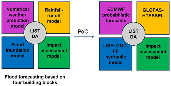
Figure 1. Overall concept of the Digital Twin for flood forecasting.

Figure 2 illustrates the diagram of the proposed flood forecasting system. In this research work, the flood forecasting strategy involves the local grid-based hydraulic model LISFLOOD-FP combined with inflow discharges provided by GloFAS streamflow forecasts. However, the daily GloFAS forecast discharge ensemble is not directly used as forcing data for the LISFLOOD-FP model. Instead, the hydrodynamic LISFLOOD-FP model is employed to compute a series of flood depth maps beforehand based on various scenario settings that account for a wide range of meteorological and hydrological conditions. The GloFAS forecast discharges are then used as a reference to identify and select the corresponding pre-computed flood depth maps, rather than serving as direct forcing data for conventional hydraulic simulations. Lastly, the DA process is implemented using a PF approach, similar to [17,68], to assimilate flood probability maps that are derived from Sentinel-1 images using GFM [72,73].

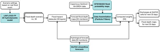
Figure 2. Diagram of the proposed method.

It is worth noting that the proposed framework is highly flexible and can be adapted to integrate different combinations of hydrological streamflow forecasts and hydrodynamic models and can be updated using various sources of flood extent observations. Furthermore, unlike conventional flood forecast systems, which require running computationally expensive hydrodynamic models each time new streamflow forecasts become available, the proposed framework adopts a pre-computation and matching retrieval paradigm. By generating a comprehensive flood hazard datacube beforehand, covering a wide range of hydrological scenarios, the forecasting stage is reduced to a matching operation between GloFAS probabilistic discharge forecasts and the most relevant pre-computed flood depth maps. The resulting efficiency not only facilitates NRT operation but also allows system robustness, scalability to larger regions, and suitability for operational early-warning systems, of which computational resources and processing time are of paramount importance.

High-resolution numerical simulations by LISFLOOD-FP (described below in Section 2.1) pre-compute maximum water depth maps for various river inflow discharge scenarios, forming a flood hazard datacube with 38 layers (described below in Section 2.2). Each layer corresponds to a specific discharge scenario, and the number of layers is associated with the number of peak discharges used by the scenarios. Using the GloFAS probabilistic discharge forecast ensemble (described below in Section 2.3), the forecast streamflow discharge is matched with the datacube at a daily time step to extract corresponding flood depth maps at 5 m resolution, generating an ensemble of flood inundation maps. Each map shall be considered a particle, representing a realization of the current studied event. When becoming available, Sentinel-1-derived flood maps (described in Section 2.4) are used to compare with the simulated flood maps from the ensemble to update the weight of the particles according to their agreement with the Sentinel-1 flood probability maps.

It is worth noting that incorporating satellite-based flood observations is a key feature of this strategy. Sentinel-1 flood observations, processed by flood mapping methods, provide NRT and reliable evidence of flood events. These satellite-based observations are particularly valuable in regions where ground-based monitoring data is sparse or even unavailable. The DA compares the flood probability maps from either GFM (called PF1) or from GFM enhanced with WASDI-based urban flood mapping [75] (called PF2) with the pre-computed flood hazard datacube generated by LISFLOOD-FP.

By integrating the GFM and GloFAS products through DA, built on top of a local LISFLOOD-FP hydrodynamic model with high-resolution outputs, the DT is capable of medium- and extended-range daily inundation forecasting up to 30 days, while reducing predictive uncertainties. The DA strategy is flexible and can accommodate various global- and local-scale models and resolutions. The PF implementation involves the weighting scheme as proposed by Di Mauro et al. [68] to deal with degeneracy and impoverishment problems. It allows weighted combinations of pre-computed flood depth maps from LISFLOOD-FP according to its agreement with flood probability maps observed by Sentinel-1.

2.1. Study Area, Data, and Hydraulic Model

2.1.1. Study Area and Gauging Station Network

The study area on the Alzette River (Luxembourg) is situated downstream of Luxembourg City, between the gauging stations at Pfaffenthal (upstream) and Ettelbruck (downstream), covering a stretch of approximately 28 km with an average slope of 0.001 m/m. This section is also fed by three tributaries: the Mamer, Eisch, and Attert Rivers. The Alzette basin was chosen because of its well-instrumented hydrometric network providing reliable in situ discharge and water level data, while it has experienced several recent significant flood events, including the extreme July 2021 flood, making it hydrologically relevant for DT development. The scale and characteristics of the river basin make it representative of small- to medium-sized river systems, potentially supporting transferability of findings. Figure 3a illustrates the model domain and river gauge network, along with the catchment topography. Green dots in Figure 3a mark the model’s four upstream BC inputs, located at Pfaffenthal (Alzette River), Schoenfels (Mamer River), Hunnebour (Eisch River), and Bissen (Attert River). The information on these gauge stations is summarized by Table 2. On the other hand, red dots in Figure 3a represent additional gauging stations within the model domain used for model calibration and validation. They are summarized by Table 3, providing discharge and water stage time series at a 15 min time step throughout the studied flood events. Beside Hunsdorf, the stations are operated by the Administration de la Gestion de l’Eau (AGE). In the context of flooding, Table A1 in Appendix A summarizes the statistical discharge and water level values at these stations according to the return period.

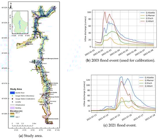
Figure 3. (a) The study area on the Alzette River (Luxembourg). The study reach is located downstream of Luxembourg City between the gauge stations at Pfaffenthal and Ettelbruck. Green solid dots represent gauge stations providing upstream BCs, whereas red solid dots represent those used for the calibration and validation. Inflow discharge for (b) 2003 and (c) 2021 flood events at Pfaffenthal (Alzette River, blue), Schoenfels (Mamer River, orange), Hunnebour (Eisch River, green), and Bissen (Attert River, red).

Table 2. Gauging stations for upstream BCs. Source: https://www.inondations.lu/ (accessed on 15 October 2025).

Name (Operator)	Water-Course	Basin Size [${\mathrm{km}}^2$]	Gauge Altitude [m.a.s.l.]	River Chainage [km]	Latitude (WGS84)	Longitude (WGS84)	Operating Since	Orange Threshold [m]	Red Threshold [m]
Pfaffenthal (AGE)	Alzette	360.5	235.25	35.04	49.6206	6.1323	1 October 1996	2.20	2.70
Schoenfels (AGE)	Mamer	83.6	222.56	3.79	49.7231	6.1008	1 September 1996	-	-
Hunnebour (AGE)	Eisch	164.2	223.48	5.33	49.7292	6.0795	1 August 1996	2.35	2.80
Bissen (AGE)	Attert	291.5	218.56	5.6	49.7849	6.0564	1 December 1996	2.50	3.0

Table 3. Gauging stations on the Alzette for calibration/validation. Source: https://www.inondations.lu/ (accessed on 15 October 2025).

Name (Operator)	Water-Course	Basin Size [${\mathrm{km}}^2$]	Gauge Altitude [m.a.s.l.]	River Chainage [km]	Latitude (WGS84)	Longitude (WGS84)	Operating Since	Orange Threshold [m]	Red Threshold [m]
Walferdange (AGE)	Alzette	405.1	225.32	28.69	49.6687	6.1301	1 November 2002	-	-
Steinsel (AGE)	Alzette	406.9	222.26	27.43	49.6785	6.1325	1 November 1996	3.0	3.50
Hunsdorf (LIST)	Alzette	410.1	220.57	24.69	49.6990	6.1336	29 June 2001	-	-
Mersch (AGE)	Alzette	707.0	212.35	16.48	49.7531	6.1160	1 August 1996	3.50	4.0
Ettelbruck (AGE)	Alzette	1091.9	193.99	1.14	49.8448	6.0986	1 September 1996	1.80	2.30

2.1.2. LISFLOOD-FP Hydrodynamic Model

LISFLOOD-FP [76] is a raster-based 2D hydrodynamic model that simulates the propagation of flood waves along channels and across floodplains using a storage cell approach. The model solves the shallow water equations (SWEs) at low computational cost by neglecting the convective acceleration term using an explicit finite difference scheme [77] while the model time step is determined by the Courant–Friedrichs–Lewy condition to ensure numerical stability [78]. A sub-grid river channel representation is introduced to allow the characterization of channel width independent of the nominal model resolution [79].

Setting up a LISFLOOD-FP model requires a DEM for floodplain topography, channel geometry (river width, depth, and shape), BCs, and Manning’s roughness coefficients n for both the channel ($n_{\mathrm{ch}}$) and floodplain ($n_{\mathrm{fp}}$). The BCs consist of upstream discharge time series at all four inflow points to the model domain and downstream WSE time series at all outflow points (Figure 3a). Three additional input data (channel width, channel depth, and bank elevation) are required for the sub-grid channel scheme. A sub-grid formulation of LISFLOOD-FP was set up in this study, with the channel of the Alzette River represented as 1D sub-grid scale features and the floodplain represented using the inertial formulation of the shallow water equations [77]. The floodplain topography and three tributaries (Mamer, Eisch, and Attert) in the model were described using the 2019 LiDAR DEM (https://data.public.lu/fr/datasets/lidar-2019-modele-numerique-de-terrain-mnt/ (accessed on 15 October 2025)) rescaled to a 5-m spatial resolution, balancing computational efficiency for multiple simulations required for the calibration process with the model ability to accurately capture floodplain inundation patterns.

The width of the 1D sub-grid channel was derived from 266 surveyed cross-section widths (https://data.public.lu/fr/datasets/cartographie-des-profils-en-travers-2021/ (accessed on 15 October 2025)), provided by the AGE within the framework of the “Cartographie des profils en travers 2021”. The DEM elevation was used to represent the bank height elevation, defining the channel bankfull depth in combination with channel bed elevation [80]. The channel geometry was assumed to be rectangular, since similar water level simulation accuracy was observed between models with rectangular channels and calibrated channel roughness and those with non-rectangular shapes [81]. Given this configuration, the channel depths in the model may differ from in situ measurements, and thus were approximated during calibration using a empirical power law formulation [79], given by $D=r_{\mathrm{ch}}\times W^{p_{\mathrm{ch}}}$ where D is the channel depth, W the channel width, and $r_{\mathrm{ch}}$ and $p_{\mathrm{ch}}$ the channel depth parameters. It is acknowledged that the rectangular channel configuration is unlikely to significantly impact the simulation results [81].

Hourly discharge data from four gauging stations on Alzette at Pfaffenthal, Mamer at Schoenfels, Eisch at Hunnebuer, and Attert at Bissen (Figure 3b,c for the 2003 and 2021 flood event, respectively) were used as the upstream BCs. On the other hand, instead of utilizing the gauging station at Ettelbruck as a downstream stage-varying BC, a free downstream BC was imposed to account for the backwater effect. It should be noted that the 2003 flood event (Figure 3b) is only used for the calibration of the LISFLOOD-FP model, based on in situ data and reference flood hazard maps. On the other hand, the 2021 flood event (Figure 3c) is the focus of the paper, demonstrating the merits of the assimilation of satellite EO data in the context of flood forecasting.

Together with the two channel depth parameters ($r_{\mathrm{ch}}$ and $p_{\mathrm{ch}}$), the Manning’s n roughness coefficients for channel ($n_{\mathrm{ch}}$) and floodplain ($n_{\mathrm{fp}}$) were also considered in the calibration process. A priori parameter distributions were assumed to be uniform due to insufficient evidence for effective parameter distributions [82,83]. The parameter ranges were determined based on their physically feasible limits and values reported in the literature. If no values were available in the literature, default values based on expert knowledge were used, with a variation of $\pm 50\%$ from the default or within ranges suggested by prior modeling experience. The Alzette River in this study area is characterized as a gravel bed, concrete banks, and a floodplain dominated by cultivated areas and brush. Therefore, to capture the full range of potential roughness values, channel roughness $n_{\mathrm{ch}}$ values were set between 0.01 and 0.05, and floodplain roughness $n_{\mathrm{fp}}$ between 0.03 and 0.15 [84]. The ranges for $r_{\mathrm{ch}}$ and $p_{\mathrm{ch}}$ were set between 0.01 and 0.15 and between 0.01 and 1.00, respectively. The distribution of these parameters are summarized in Table 4. Latin hypercube sampling [85] was employed to enhance the efficiency of Monte Carlo sampling, ensuring effective coverage of parameter interactions in multiple dimensions while generating minimally correlated parameter sets from a sparse sample size [86]. In total, 500 parameter sets were generated for this study.

Table 4. Distribution for LISFLOOD-FP model parameters.

Parameter	Distribution
Channel depth $r_{\mathrm{ch}}$	$\mathcal{U}\left(0.01;0.15\right)$
Channel depth $p_{\mathrm{ch}}$	$\mathcal{U}\left(0.01;1.00\right)$
Channel roughness $n_{\mathrm{ch}}$	$\mathcal{U}\left(0.01;0.05\right)$
Floodplain roughness $n_{\mathrm{fp}}$	$\mathcal{U}\left(0.03;0.15\right)$

Two observed datasets were used for model assessment: (1) Stage data from the Walferdange and Steinsel stations and discharge data from the Hunsdorf, Mersch, and Ettelbruck stations; (2) A flood inundation extent map extracted from the Sentinel-1 satellite imagery. The model performance in reproducing the timing and magnitude of the January 2003 flood event was evaluated against the gauging stations using the Kling–Gupta efficiency (KGE) [87], defined in Section 2.6.1, while its ability to capture the flood inundation extent of the July 2021 flood event was assessed by comparing against the observed flood extent map and calculating the Critical Success Index ($\mathrm{CSI}$). Based on a combination of $\mathrm{KGE}$ and $\mathrm{CSI}$ results, the parameter sets were ranked and normalized into generalized conditional probabilities [86]. The observed datasets were combined by evaluating on one dataset and using the other to update the weights for each parameter set through a recursive application of Bayes’ equation [86]. The parameter set associated with the highest combined conditional probability values was selected as the best parameter set for generating the water depth and flood inundation extent maps.

2.2. Scenario Generation

As aforementioned, in order to carry out the proposed method, a flood hazard datacube is necessary. A total of 38 scenarios were generated with the calibrated LISFLOOD-FP model based on the 2021 flood hydrograph scaled to different maximum discharge values at the four BCs. Each scenario reflects a different flow condition, allowing for a comprehensive analysis of hydrodynamic behavior across a wide range of potential discharge rates. The scenarios provide a detailed spectrum of flow responses for various hydraulic conditions, enabling accurate assessments of system performance under both low- and high-flow events. For instance, peak discharge values at Pfaffenthal, represented by $Q_{max}$, range from 5 to 190 ${\mathrm{m}}^3$·${\mathrm{s}}^{-1}$ with an increment of 5 ${\mathrm{m}}^3$·${\mathrm{s}}^{-1}$. The four BCs (Table 2) were matched based on their associated return periods (summarized by Table A1 in Appendix A). Each of the 38 scenarios corresponds to one return period and one unique set of $Q_{max}$ values across the four BCs, as shown in Figure 4. The appropriate scenario is selected based on the forecasted $Q_{max}$ at Pfaffenthal from GloFAS. Using these scaled hydrographs as input, the LISFLOOD-FP model produces pre-computed water depth maps (Figure 5), which together form the flood hazard datacube. Figure 5 illustrates four sample scenarios, ranging from the lowest to the highest return period scenarios.

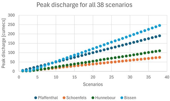
Figure 4. Peak discharge for all 38 scenarios for all four BCs.

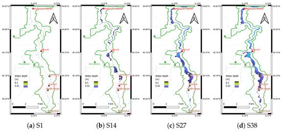
Figure 5. Pre-computed 5 m resolution flood depth maps for different inflows using LISFLOOD-FP model. From left to right: four scenarios: S1 (peak discharge at Pfaffenthal: 5 ${\mathrm{m}}^3$·${\mathrm{s}}^{-1}$), S14 (peak discharge at Pfaffenthal: 70 ${\mathrm{m}}^3$·${\mathrm{s}}^{-1}$), S27 (peak discharge at Pfaffenthal: 135 ${\mathrm{m}}^3$·${\mathrm{s}}^{-1}$), and S38 (peak discharge at Pfaffenthal: 190 ${\mathrm{m}}^3$·${\mathrm{s}}^{-1}$). Green lines represent the hydraulic model domain.

2.3. Hydrological Rainfall–Runoff Model—GloFAS Streamflow Forecasts

GloFAS, within the CEMS, has been pre-operational since 2011 and fully operational since April 2018. Its hydrological modeling components include the land surface model of ECMWF IFS, H-TESSEL [88], and the open-source LISFLOOD (https://ec-jrc.github.io/lisflood/ (accessed on 15 October 2025)) hydrological model [89]. To produce and predict global river discharge [71], GloFAS uses medium- and extended-range meteorological forecasts from ECMWF-ENS as forcing data to the LISFLOOD, to provide publicly available ensemble real-time daily forecasts for the next 30 days for its global river network. More information can be found in Appendix B.

This gridded dataset offers a consistent representation of key hydrological variables across the global domain, namely river discharge, soil wetness index (root zone), snow water equivalent, runoff water equivalent (surface plus sub-surface). We utilize the 24 h averaged river discharge, representing the volumetric flow rate passing through a river cross-section over the specified time step. In this research work, we rely on the GloFAS streamflow forecast dataset (version 3.1) with a spatial resolution of ${0.1}^{°}\times {0.1}^{°}$ [71]. Although GloFAS provides dicharges at daily temporal resolution, which may smooth short-term discharge variability, it remains the preferred forcing dataset in this study due to its global coverage, operational availability, and proven skill in providing reliable medium- to extended-range streamflow forecasts. Figure 6 illustrates the daily GloFAS streamflow forecasts, generated with 50 ensemble members, starting from one of four issuing dates: 12 July 2021 (first panel), 13 July 2021 (second panel), 14 July 2021 (third panel), and 15 July 2021 (last panel). It is important to note that each forecast begins with day 1 following its issuance (e.g., the 12 July forecast corresponds to 13 July as day 1). From the top two panels (12 July and 13 July forecasts), it can be observed that the ensemble spread widens as the flood event begins and remains substantial throughout the recession phase. It should also be noted that the 15 July forecasts (day 1 starting from 16 July) in Figure 6 mark the recession of the flood event, and, therefore, they will not be included in the implementation of the proposed method.

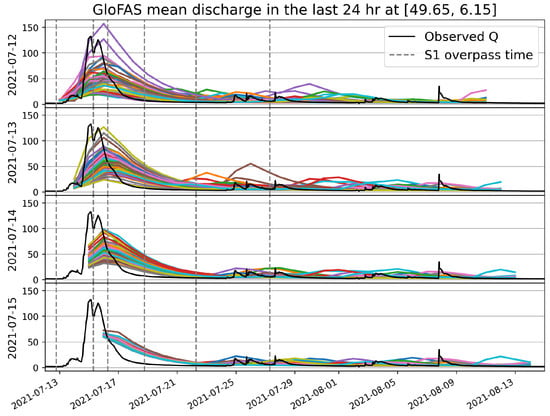
Figure 6. GloFAS streamflow forecasts issued on 12 July (first panel), 13 July (second panel), 14 July (third panel), and 15 July (fourth panel). Observed discharge (black lines) and 50 forecasted daily discharges (colored lines). The overpass times of Sentinel-1 SAR are indicated with vertical dashed lines.

2.4. Flood Extent Mapping with GFM

Sentinel-1, a Copernicus constellation [90] of two polar-orbiting satellites, operates day and night performing C-band SAR imaging regardless of the weather conditions. Based on the systematic stream of Sentinel-1 data, NRT GFM product can be provided for the CEMS [72] within less than eight hours after image acquisition. The product is obtained by an ensemble approach combining the results of three independently developed flood mapping methods by [74,91,92].

Sentinel-1 data are collected in Interferometric Wide-swath mode with Ground Range Detected at High resolution (Sentinel-1 IW GRDH). The GRD products include focused SAR data that has been detected, multi-looked, and projected to ground range using an Earth ellipsoid model, with phase information discarded. This results in a product with approximately square pixels and spacing, offering reduced speckle but at the cost of lower spatial resolution. In this case, the raw backscatter amplitude is sampled with a pixel size of $10\times 10$ m. Only VV-polarization data are used here due to their superior sensitivity in distinguishing water from non-water surfaces.

The preprocessed Sentinel-1 output is formatted as Analysis-Ready-Data, which is then sent to the GFM flood detection engine. Here, three algorithms run concurrently to generate NRT flood mapping products. The GFM product relies on an ensemble approach that combines three well-established, independently developed flood detection algorithms from LIST [74], the German Aerospace Center (DLR) [91], and Vienna University of Technology (TUW) [92]. The flood ensemble is calculated pixel by pixel using a majority voting system, where at least two of the algorithms must classify a pixel as flooded or non-flooded [93].

A second flood extent mapping method [75] was also integrated into this study to improve the detection of floodwater in urban areas compared to GFM. This approach exploits Interferometric SAR coherence to identify inundation within built environments and is accessible via the WASDI platform (https://www.wasdi.net/#/edrift_auto_urban_flood/appDetails (accessed on 15 October 2025)). In this work, the PF2 experiment incorporates combined flood probability maps derived from both GFM and the WASDI-based urban flood detections, hereafter referred to as GFM + WASDI in the subsequent sections.

2.5. Data Assimilation with Particle Filters

This section establishes the DA framework for integrating SAR-derived flood probability maps within the flood forecasting model built around the hydrodynamic LISFLOOD-FP model. Using the ensemble of GloFAS streamflow forecasts (comprising of 50 members) to match with the upstream BCs devised for each scenario, a 50-member ensemble of water depth maps is extracted from the pre-computed flood hazard datacube. An ensemble of binary maps is then generated where each pixel is classified as either wet or dry, using a 10 cm threshold of water depth. The wet/dry binary map is then compared against the flood probability map derived from a SAR image (in this study, from Sentinel-1 images processed by GFM/GFM + WASDI algorithms). To optimally combine observations and simulations, we adopt a PF approach. PFs are advantageous with fully non-linear DA as they relax the assumption of Gaussian errors [94]. In addition, the implementation of the SIS, inspired by Hostache et al. [17], offers the advantage of preventing updates to model states that could potentially cause instabilities in the hydraulic model. The prior and posterior probability distributions, representing model states across the model grid cells before and after an assimilation, are approximated using a set of N particles. Each of them corresponds to the output from the forecast model (through GloFAS streamflow forecast and LISFLOOD-FP), with its own set of uncertainties and a weight, which indicates the likelihood of that specific model output being correct according to the observation. During an assimilation, the PF analysis ascribes the particle weights based on flood information from the Sentinel-1-derived flood probability data resulted from GFM.

The DA framework involves two key steps: the forecast step, where model simulations are performed, and the analysis step, during which the weights of N particles $\{x^1,x^2,\dots ,x^N\}$ are updated based on available observations. The relationship between the observation vector y (i.e., the observed flooded/non-flooded pixels) and the true state $x^t$ is expressed as $y=\mathcal{H}\left[x^t\right]+ϵ$ where $\mathcal{H}$ is the observation operator, and $ϵ$ represents observation errors.

At any given time step k, the prior PDF of the model state x is described by a set of N independent random particles $x^n$:

$$p_k\left(x\right)\approx \sum _{n=1}^N{\mathrm{\Theta }}_k^n\delta \left(x-x_k^n\right),$$

(1)

where $\delta \left(z\right)$ is the Dirac delta function (which is zero everywhere except for z; its integral is equal to one), and the initial weights ${\mathrm{\Theta }}_k^n$ are assumed to be uniform (i.e., ${\mathrm{\Theta }}_k^n=1/N$, for $n=1,\dots ,N$).

At the forecast step, the model (denoted by $\mathcal{M}$) propagates the particles without approximation:

$$p_{k+1}\left(x\right)\approx \sum _{n=1}^N{\mathrm{\Theta }}_k^n\delta \left(x-x_{k+1}^n\right) \mathrm{with} x_{k+1}^n={\mathcal{M}}_{k+1}\left(x_k\right).$$

(2)

The analysis step updates the weight of each particle according to the likelihood of the particle given the observation:

$${\mathrm{\Theta }}_{k+1}^{a,n}\propto {\mathrm{\Theta }}_{k+1}^{f,n}p\left(y_{k+1}|x_{k+1}^n\right),$$

(3)

where superscript a stands for analysis, and superscript f stands for forecast.

Similar to existing works [17,32], here the likelihood (global weight, ${\mathrm{\Theta }}^n$ for particle $n=1,\dots ,N$) is computed by the product of the pixel-based likelihoods (local weights ${\theta }_i^n$ for pixel $i=1,\dots ,L$ of member n), assuming that the L pixel observation errors are independent from each other. At time k of the observation, local weights ${\theta }_{i,k}^n$ are defined for each particle n and for each pixel i according to [17]:

$${\theta }_{i,k}^n=p_{i,k}\left(\mathcal{W}|{\sigma }_0\right)\times M_{i,k}^n+\left[1-p_{i,k}\left(\mathcal{W}|{\sigma }_0\right)\right]\times \left(1-M_{i,k}^n\right),$$

(4)

where $p_i\left(\mathcal{W}\right|{\sigma }_0)$ represents the probability of a pixel being classified as wet ($\mathcal{W}$) based on the Sentinel-1 observations, and $\{1-p_i\left(\mathcal{W}\right|{\sigma }_0)\}$ represents the probability of it being classified as dry. $M_{i,k}^n$ is set to “1” if the model predicts the pixel as wet and “0” if the model predicts it as dry. The simulated water depth maps are transformed into binary flood extent maps by treating a pixel as wet if the water level exceeds 10 cm. Applying Equation (4) assigns higher probabilities to pixels where model predictions align with observations. It is worth emphasizing that Equation (4) fundamentally evaluates the pixel-wise consistency between the simulated and observed flood extents. It quantifies how likely it is that a given model realization correctly reproduces the observed flood condition at that pixel, thereby forming the basis of the particle weight calculation. These local pixel-wise likelihoods are subsequently aggregated across the full spatial domain to obtain the global weight of each particle. As such, ${\mathrm{\Theta }}^n$ is computed by the normalized product of local weights, ensuring that the sum of global weights equals 1, as follows:

$${\mathrm{\Theta }}^n={\displaystyle \frac{{\prod }_{i=1}^L{\theta }_{i,n}}{{\sum }_{n=1}^N\left({\prod }_{i=1}^L{\theta }_{i,n}\right)}}.$$

(5)

As suggested by Hostache et al. [17], such a spatial aggregation is implemented to avoid assigning a weight of zero to an otherwise plausible particle solely due to local mismatches, as well as to alleviate bias arising from the tendency of false positives (overestimated flooded areas) being penalized more strongly than underpredicted areas. Additionally, unless the number of particles N increases exponentially with the dimensionality of the system state, the PF is prone to degeneration [69], as a high probability is often concentrated in a single particle, leaving the rest with minimal weights [94]. PFs commonly face such degeneration issues, particularly when N is insufficient due to computational constraints [95]. Following the application of a standard PF, weight variance typically increases, causing only a few particles to retain significant weight. To address this issue, we apply here the adaptation on the global weight from Equation (5) proposed by Hostache et al. [17], using a tempering coefficient $\alpha$, as shown in the following Equation:

$${\mathrm{\Theta }}_n\left(\alpha \right)={\displaystyle \frac{{\prod }_{i=1}^L{\theta }_{i,n}^{\alpha }}{{\sum }_{n=1}^N\left({\prod }_{i=1}^L{\theta }_{i,n}^{\alpha }\right)}}.$$

(6)

In this study, the coefficient $\alpha$ was selected following the rationale proposed by [68]. The resulting global weights are used to estimate the water levels (H) and discharge (Q) at time k and per pixel i (for H) or per GloFAS grid j (for Q), as follows:

$${\overline{H}}_i=\sum _{n=1}^N{\mathrm{\Theta }}^n·H_i^n,$$

(7)

$${\overline{Q}}_j=\sum _{n=1}^N{\mathrm{\Theta }}^n·Q_j^n.$$

(8)

It should be noted that while the water levels H are pixel-based following the datacube resolution, the discharge estimates Q are only available at GloFAS grid cells. The particles retain their global weights until the next assimilation step. Afterward, all particles are reset to an equal weight before a new analysis step begins. In contrast, the expectation in the Open Loop (OL), i.e., without DA, is simply the ensemble mean, as each particle holds the same relative importance.

2.6. Performance Metrics

2.6.1. 1D Metrics for Water Level and Discharge Time-Series Assessment

The quality of the simulated water level $H^m$ (respectively, discharge $Q^m$) is assessed with respect to in situ observations $H^o$ (respectively, discharge $Q^o$) in terms of root-mean-square error ($\mathrm{RMSE}$), Kling–Gupta efficiency ($\mathrm{KGE}$) [87], and the Nash–Sutcliffe model efficiency coefficient ($\mathrm{NSE}$) [96] over the flood event. $\mathrm{RMSE}$ is computed between the simulated and the observed WL time series, sampled at observation times, for the entire flood event:

$$\mathrm{RMSE}=\sqrt{{\displaystyle \frac{1}{n_{obs}}}\sum _{i=1}^{n_{obs}}{(H_i^m-H_i^o)}^2}$$

(9)

On the other hand, $\mathrm{NSE}$ reflects on the ratio of the error variance of the simulated time series divided by the variance of the observed time series:

$$\mathrm{NSE}=1-{\displaystyle \frac{{\sum }_{i=1}^{n_{obs}}{(H_i^m-H_i^o)}^2}{{\sum }_{i=1}^{n_{obs}}{(H_i^o-\overline{H^o})}^2}}$$

(10)

where $\overline{H^o}$ denotes the time-averaged observed water level over the event. For a perfect model, the estimation error variance computed with respect to observation is equal to 0 (i.e., ${\sum }_{i=1}^{n_{obs}}{(H_i^m-H_i^o)}^2=0$), thus the resulting $\mathrm{NSE}$ is equal to 1. Resulting $\mathrm{NSE}$ values nearer to 1 suggest a model with greater predictive capacity. A model that produces an estimation error variance equal to the variance of the observed time-series results in a $\mathrm{NSE}$ equal to 0. Furthermore, when the estimation error variance computed with respect to observation is larger than the variance of the observations, the $\mathrm{NSE}$ becomes negative. In other words, a negative $\mathrm{NSE}$ occurs when the observed mean is a better predictor than the model.

Lastly, $\mathrm{KGE}$ is a statistical metric widely adopted in hydrology and water resources engineering to evaluate model performance in simulating streamflow, groundwater recharge, and water quality parameters. It was introduced to address the shortcomings of other metrics, e.g., the $\mathrm{NSE}$ and the coefficient of determination (${\mathrm{R}}^2$), which primarily focus on replicating the mean and variance of observed data. The $\mathrm{KGE}$ combines three components: the Pearson correlation coefficient (r), the variability ratio ($\gamma$), and the bias ratio ($\beta$), providing a comprehensive evaluation of model performance:

$$\mathrm{KGE}=1-\sqrt{{\left[1-r(H^m,H^o)\right]}^2+{\left[1-\beta (H^m,H^o)\right]}^2+{\left[1-\gamma (H^m,H^o)\right]}^2}$$

(11)

$$r(H^m,H^o)={\displaystyle \frac{\mathrm{cov}({\mathrm{H}}^{\mathrm{o}},{\mathrm{H}}^{\mathrm{m}})}{\mathrm{std}\left(H^o\right)\mathrm{std}\left(H^m\right)}}$$

(12)

$$\beta (H^m,H^o)={\displaystyle \frac{\mathrm{mean}\left(H^m\right)}{\mathrm{mean}\left(H^o\right)}}$$

(13)

$$\gamma (H^m,H^o)={\displaystyle \frac{\mathrm{std}\left(H^m\right)/\mathrm{mean}\left(H^m\right)}{\mathrm{std}\left(H^o\right)/\mathrm{mean}\left(H^o\right)}}$$

(14)

The $\mathrm{KGE}$ value ranges from negative infinity to 1, with 1 representing a perfect match between model predictions and observed data. It not only evaluates the accuracy of predictions but also considers the model’s ability to capture the variability and timing of observed data.

2.6.2. 2D Metrics for Flood Extent Assessment

In order to assess the comparison between the simulated and the observed flood extents, the $\mathrm{CSI}$ (Critical Success Index) is used. $\mathrm{CSI}$ evaluates the simulated flood extent maps based on the ground truth that is the observed flood maps. These indices are based on the count of pixels in one of four possible outcomes, forming a contingency map: True Positives ($TP$s, or hits) represent the number of correctly predicted flooded pixels, while True Negatives ($TN$s) denote the correctly identified non-flooded pixels. False Positives ($FP$s, or false alarms), also known as over-prediction, refer to non-flooded pixels incorrectly predicted as flooded, and False Negatives ($FN$s, or misses), also called under-prediction, represent flooded pixels that were not correctly identified.

$$\mathrm{CSI}={\displaystyle \frac{TP}{TP+FP+FN}}.$$

(15)

This metric ranges from 0% when there is no common area (i.e., no agreement) between the simulated and the observed flood extents to their highest value of 100% when the prediction provides a perfect fit to the observed flood extents.

3. Results and Discussion

3.1. Evaluation of LISFLOOD-FP Hydraulic Model Component

3.1.1. Model Performance over the Calibrating 2003 Flood Event

It is worth noting that an initial assessment of the LISFLOOD-FP model calibration revealed that the model tended to have over-prediction around the urban areas between Walferdange and Steinsel. This shows that a uniform parameterization could not adequately represent the hydraulic variability of the domain. As such, the model domain was divided into two regions, namely the first region between Pfaffenthal and Hunsdorf and the second region between Hunsdorf and Ettelbruck, such that two different parameter sets were sampled in these two regions during the calibration process. Table 5 shows the 1D metrics $\mathrm{KGE}$ and $\mathrm{NSE}$ computed over the 2003 flood event between the simulated water levels/discharges and the observed ones at the gauge stations. After the re-calibration, the model generally shows a satisfactory performance with $\mathrm{KGE}$ above 0.95 at all observing stations for the 2003 flood event. Figure 7 reveals the simulated water levels at Walferdange and Steinsel and the simulated discharges at Hunsdord, Mersch (Beringen), and Ettelbruck in red lines, against the observed water levels/discharges in blue lines. It should be noted that the observed discharges at Hunsdorf station were discontinued for a couple of hours during the flood peak due to a technical problem. Nevertheless, the rising and falling limbs of all the hydrographs are well produced, capturing the timing of both flood onset and recession accurately. The peak discharges also show good agreement with the observed, despite a slight tendency of the model to overpredict at Steinsel and Mersch station. Overall, the LISFLOOD-FP model performs rather well across the entire domain, demonstrating its effectiveness in representing hydrological variations and dynamics.

Table 5. NSE and KGE—2003 flood event (used for calibration).

	Walferdange (H)	Steinsel (H)	Hunsdorf (Q)	Mersch (Q)	Ettelbruck (Q)
$\mathrm{KGE}$	0.97	0.97	0.97	0.94	0.95
$\mathrm{NSE}$	0.96	0.51	0.95	0.82	0.89

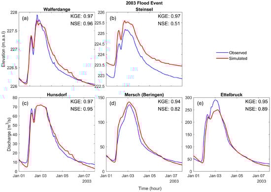
Figure 7. Observed (blue line) and simulated (red line) water levels during 2003 flood event at (a) Walferdange and (b) Steinsel stations, and discharges at (c) Hunsdorf, (d) Mersch, and (e) Ettelbruck stations.

Figure 8 shows the contingency map between the simulated flood extent and Sentinel-1 observed flood extent maps, overlaid over the topography data. Hit (grey) means the pixel is flooded in both the simulation and observation, Miss (blue) means the pixel is flooded in the observation but not in the simulation, and False Alarm (red) means the pixel is flooded in the simulation but not in the observation. A pixel that is not flooded in both the simulation and observation is not shown for visual clarity.

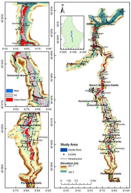
Figure 8. Model performance against the Sentinel-1 satellite imagery over the study reach in terms of the contingency map for the 2021 flood event. Green solid dots represent gauge stations whereas blue dots represent the localities.

Evaluating against the satellite-derived water extent also shows some regions of over-prediction such as urban areas between Pfaffenthal and Steinsel and the river channel between Mersch and Ettelbruck (Figure 8), which result in a $\mathrm{CSI}$ of 0.49. However, it is acknowledged that these over-predictions could be due to the inability of Sentinel-1 to observe water bodies in narrow river channels and the difficulty in water detection in built-up areas.

3.1.2. Model Performance over 2021 Flood Event

As aforementioned, the 2003 flood event was used for calibrating the LISFLOOD-FP model, whereas the 2021 flood event serves as the main case study, illustrating the effectiveness of assimilating satellite-based EO data to enhance flood forecasting performance. Similar to Table 5, Table 6 presents the 1D metrics $\mathrm{KGE}$ and $\mathrm{NSE}$ calculated for the 2021 flood event, comparing simulated water levels and discharges with the observed values at the gauge stations. Although these 1D metrics are slightly lower (i.e., reduced $\mathrm{KGE}$ and $\mathrm{NSE}$) compared to those in Table 5 from the calibration period, they remain within a high range, with $\mathrm{KGE}$ values all exceeding 0.82 and $\mathrm{NSE}$ values above 0.64. This is further supported by the visual comparison shown in Figure 9, which contrasts the simulated water levels at Walferdange and Steinsel, and the simulated discharges at Hunsdrof, Mersch (Beringen), and Ettelbruck (red lines), with the observed water levels and discharges (blue lines). Compared with the calibrated 2003 flood, the 2021 event was a summer flood characterized by intense precipitation concentrated over the Alzette valley, leading to distinct hydrometeorological and antecedent wetness conditions.

Table 6. NSE and KGE—2021 flood event.

	Walferdange (H)	Steinsel (H)	Hunsdorf (Q)	Mersch (Q)	Ettelbruck (Q)
$\mathrm{KGE}$	0.96	0.82	0.86	0.92	0.94
$\mathrm{NSE}$	0.88	0.54	0.62	0.70	0.84

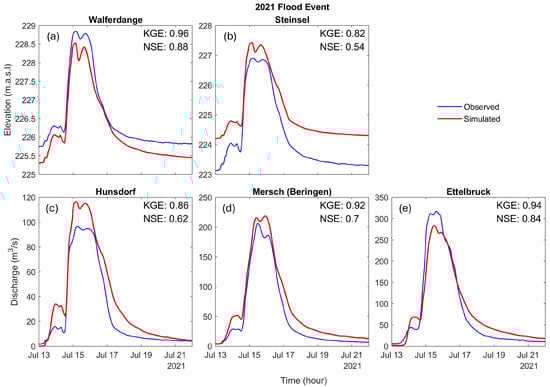
Figure 9. Observed (blue line) and simulated (red line) water levels during 2021 flood event at (a) Walferdange and (b) Steinsel stations, and discharges at (c) Hunsdorf, (d) Mersch, and (e) Ettelbruck stations.

The flood peak of the 2021 event was captured by Sentinel-1 on its descending orbit 37 on 15 July 2021, at 05:50:52Z, and again the following day on its descending orbit 139 at 05:42:17Z on 16 July 2021. Figure 10 shows the resulting flood probability maps (left panel) generated by GFM from these Sentinel-1 images, as well as contingency maps comparing the flood probability maps (using a 35% flood probability threshold) with the simulated flood extent maps from the LISFLOOD-FP model. It is important to note that permanent water bodies are excluded from the GFM flood probability maps, which results in rivers and tributaries appearing as over-predicted areas. Overall, the central region between Steinsel and Mersch (Beringen) shows strong agreement between the simulated and observed flood extents. On 15 July, the hydrodynamic model displayed several areas of under-prediction (marked in yellow) between Pfaffenthal and Steinsel, which were no longer present on 16 July. However, these areas are categorized as low certainty in the GFM flood probability maps. Conversely, significant over-prediction (marked in red) was observed between Mersch (Beringen) and Ettelbruck on both dates, likely resulting from the narrowness of the floodplain, potential radar shadowing effects in Sentinel-1 SAR imagery, and the presence of dense riparian vegetation that hampers the sensor’s ability to detect floodwaters beneath the canopy. Previous studies show that C-band SAR often fails to detect floodwater beneath dense vegetation due to signal attenuation and scattering, leading to systematically underestimated inundation in vegetated floodplains [23,97]. To further assess model performance, comparisons were made against reference flood hazard maps for 10-year and 100-year events (Appendix C). These maps, produced using an independent hydraulic modeling setup, are not subject to the same vegetation-related detection limitations as Sentinel-1-derived flood extents. Consequently, the absence of such undetected floodwater in vegetated areas is evident in Figure A2, confirming the LISFLOOD-FP model performance.

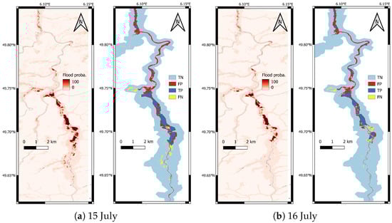
Figure 10. LISFLOOD-FP hydrodynamic model performance against the Sentinel-1-derived flood extent map observed on (a) 15 July 2021 05:50:52Z and (b) 16 July 2021 05:42:17Z. Left panels: Sentinel-1-derived flood probability maps from GFM; right panels: contingency maps between simulated and observed flood extent maps.

3.2. Evaluation of Sentinel-1-Based DA Framework

At the core of this proposed DT dedicated to flood forecasting is the use of PF, a DA technique that enables dynamic model updates based on observational data. In this study, we assess the performance of assimilating Sentinel-1-derived flood probability maps, processed by two methods: GFM alone, and GFM enhanced with WASDI-based urban flood mapping, using the same PF framework. These correspond to two distinct experiments, referred to as PF1 and PF2, respectively. It is important to note that the OL experiment represents a forecast that is the non-weighted mean of the 50 particles.

Table 7 presents the $\mathrm{RMSE}$ values calculated over a 30-day period for the 2021 flood event, comparing the simulated water levels from the OL, PF1, and PF2 experiments with the observed water levels at the Hunsdorf and Steinsel gauge stations. These two stations are selected because the flood extent assessment (Section 3.1.2) showed strong agreement between the model simulations and the observed flood maps from Sentinel-1. Similarly, Table 8 shows the $\mathrm{NSE}$s computed over time for the 2021 flood event and for the simulated inflow/outflow discharges from the OL, PF1, and PF2 experiments, with respect to the observed discharges at Pfaffenthal (the upstream BC) and Ettelbruck (the downstream BC). The PFs are applied using the GloFAS streamflow forecasts that were issued on three consecutive days, 12 July, 13 July, and 14 July, to target the flood event that reached its peak on 15 July. For each observing station, the best metrics (i.e., lowest $\mathrm{RMSE}$ and highest $\mathrm{NSE}$) are boldfaced in Table 7 and Table 8. The quantitative assessments show that all three experiments, even the OL, yield accurate water level forecasts over the next 30 days. Indeed, the relatively low $\mathrm{RMSE}$ (under 20 cm) and high $\mathrm{NSE}$ (above 0.5) from the OL demonstrate the performance of the overall approach, including the quality of GloFAS streamflow forecasts, even without the PF (that updates the weights among the particles), which combines the ensemble GloFAS streamflow forecasts and the hydraulic component.

Table 7. RMSE [m] of forecast water level over next 30 days at gauge station Hunsdorf and Steinsel. The best (lowest) $\mathrm{RMSE}$ is boldfaced.

	GloFAS Forecast Issue Date
	12 July			13 July			14 July
Exp.	OL	PF1	PF2	OL	PF1	PF2	OL	PF1	PF2
Hunsdorf	0.179	0.151	0.151	0.191	0.127	0.127	0.206	0.143	0.144
Steinsel	0.181	0.141	0.139	0.145	0.106	0.104	0.130	0.103	0.102

Table 8. NSE [-] of forecast discharge over next 30 days at gauge station Pfaffenthal (upstream BC) and Ettelbruck (downstream BC). The best (highest) $\mathrm{NSE}$ is boldfaced.

	GloFAS Forecast Issue Date
	12 July			13 July			14 July
Exp.	OL	PF1	PF2	OL	PF1	PF2	OL	PF1	PF2
Pfaffenthal	0.618	0.711	0.718	0.551	0.752	0.760	0.587	0.763	0.767
Ettelbruck	0.570	0.663	0.669	0.509	0.661	0.671	0.631	0.740	0.743

It is also shown that all DA experiments succeed in reducing the errors on the simulated water levels (i.e., $\mathrm{RMSE}$ under 15 cm) and discharge (i.e., $\mathrm{NSE}$ above 0.66) compared to those of OL. Indeed, the integration of satellite EO data (with Sentinel-1-derived flood probability maps) in both PF1 and PF2 allows for an average improvement of 15–33% for $\mathrm{RMSE}$ at Hunsdorf and Steinsel, as well as an improvement of 15–36% for $\mathrm{NSE}$ at Pfaffenthal and Ettelbruck by both PF1 and PF2. It should be noted that PF1 and PF2 yield very similar results. This is due the fact that only the flood probability maps on 15 July 2021 05:50:52Z presents a difference with an overflow in urban areas, from which PF2 is more accurate than PF1 with GFM. Indeed, although the WASDI-based refinement improves the flood mapping result in urban areas, its overall influence on basin-scale metrics remains limited for this specific event, due to small proportion of urban overflow areas within the study domain. The least improvements (from OL to PFs) were observed with only a 15% reduction in $\mathrm{RMSE}$ and a 15% increase in $\mathrm{NSE}$ when using the forecast issued on 12 July in both quantitative assessments. In contrast, the most significant improvements were achieved with the forecast issued on 13 July, indicating that a two-day lead time offers a balance between GloFAS ensemble spread and overall forecast uncertainty, where sufficient diversity among ensemble members enhances the likelihood of capturing the observed flood dynamics.

Figure 11 depicts the daily forecast water levels compared to the observed water level at observing stations: (a) Hunsdorf and (b) Steinsel, up to 30-day lead time; whereas Figure 12 reveals the forecast discharge at (a) Pfaffenthal and (b) Ettelbruck. The OL forecasts are depicted with blue crosses, while the PF1 and PF2 resulting forecasts are shown with red circles and green squares, respectively. The black lines represent the continuous observed water levels and discharges at the stations. At each Sentinel-1 overpass, the PFs successfully update the particles to align with the observations. This is evident as the water levels and discharges, shown by red circles (PF1) and green squares (PF2), move closer to the observed water levels and discharges at the various observing stations (black lines). After each assimilation times, the PFs hold the same weights for the 50 particles until the next Sentinel-1 overpass. This results in the over-predictions of water levels and discharges after the flood peak until 18 July (third vertical dashed lines). However, it is worth noting that the flood peaks at all stations were under-predicted in all three experiments. This highlights a limitation of the proposed approach, stemming from the daily resolution of the GloFAS discharge forecasts (Figure 6), which proves insufficient to produce accurate results in this case.

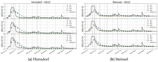
Figure 11. Forecast water levels over 30 days by OL (blue crosses) and by assimilation of GFM flood maps (red circles) and GFM with WASDI-based urban flood maps (green squares) compared to the observed water levels (black line) at (a) Hunsdorf and (b) Steinsel, using GloFAS streamflow forecasts issued on 12 July 2021 (top panels), 13 July 2021 (middle panels), and 14 July 2021 (bottom panels). Sentinel-1 overpass times are indicated as vertical dashed lines.

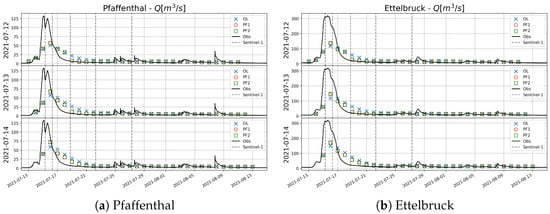
Figure 12. Forecast discharges over 30 days by OL (blue crosses) and by assimilation of GFM flood maps (red circles) and GFM with WASDI-based urban flood maps (green squares) compared to the observed discharges (black line) at (a) Pfaffenthal and (b) Ettelbruck, using GloFAS streamflow forecasts issued on 12 July 2021 (top panels), 13 July 2021 (middle panels), and 14 July 2021 (bottom panels). Sentinel-1 overpass times are indicated as vertical dashed lines.

Similar to Figure 10, Figure 13 and Figure 14 show the contingency maps for the three forecast experiments compared to the Sentinel-1-derived flood maps on 15 July 2021, at 05:50:52Z, and on 16 July 2021, at 05:42:17Z, respectively. Here, only the results using GloFAS forecasts issued on 13 July were shown. Compared to simulations driven by observed inflow discharges, these forecasts exhibit a notably lower agreement with the observed flood maps. In contrast to the 1D quantitative results, the contingency maps in Figure 13 reveal that PF1 and PF2 perform slightly worse than the OL case, showing more areas of under-prediction near Hunsdorf, although with fewer over-predictions in the northern part of the domain. Meanwhile, Figure 14 indicates minimal differences between the OL and the two PF experiments. The underperformance of the PFs relative to OL arises from the global weight computation performed using every pixel across the entire domain, which may have caused the PFs to favor suboptimal scenarios when assimilating imperfect GFM flood maps—particularly in areas affected by radar shadowing or dense vegetation, where flood extent is often underestimated. This underscores the need for a more localized weighting approach that prioritizes reliable flooded areas and employs exclusion maps [97] to mitigate these limitations.

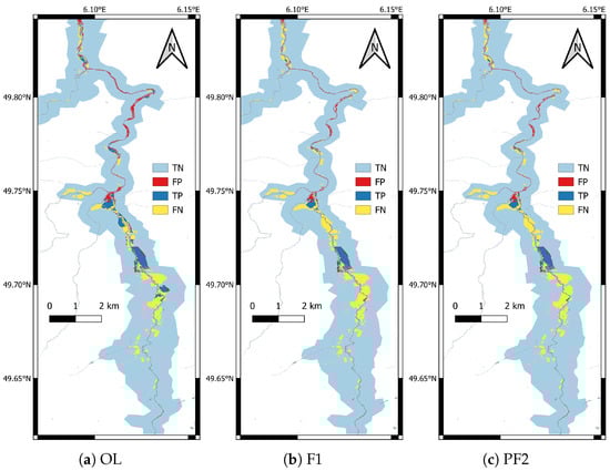
Figure 13. Assessment against Sentinel-1 flood extent map observed on 15 July 2021 05:50:52Z using GloFAS forecasts issued on 13 July 2021.

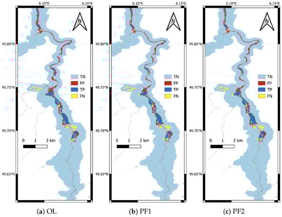
Figure 14. Assessment against Sentinel-1 flood extent map observed on 16 July 2021 05:42:17Z using GloFAS forecasts issued on 13 July 2021.

3.3. Remarks on Uncertainty of GloFAS Streamflow Forecasts

Unavoidably, the uncertainty of GloFAS streamflow forecasts plays a significant role in influencing the accuracy of flood predictions. To provide discharge forecasts used in this research work, GloFAS relies on medium- and extended-range meteorological inputs, which inherently carry uncertainties. These uncertainties tend to be more pronounced at longer lead times, where the spread of forecasted discharge across ensemble members increases, as shown in Figure 6. A key limitation of GloFAS lies in the difficulty of accurately characterizing and parameterizing these uncertainties during extreme flood events. For instance, situations may arise where the “true” discharge falls outside the ensemble spread, in which case the PF approach described here is unable to compensate for the resulting bias. In this regard, gauge data can be used to reduce systematic errors in the GloFAS forcing through post-processing with bias correction or nudging strategies, in which ensemble discharge trajectories are adjusted based on available in situ observations [70]. Such approaches would help reduce discharge forecast bias (potentially related to meteorological forecasts) and timing errors and increase the robustness of the datacube retrieval relying on GloFAS discharge, particularly during atypical or poorly represented events.

The daily discharge of GloFAS averaged over the last 24 h is also a limitation for real-time flood forecasting since it smooths out variations in river discharge, potentially missing crucial short-term fluctuations. This likely contributed to the systematic underestimation of peak flows observed across all experiments (OL, PF1, and PF2), as shown in Figure 12. Flood events often involve rapid changes in river discharge that can occur within hours, not days. By using discharge estimates averaging over a 24 h period, critical peaks in discharge that may signal imminent flooding could be missed or delayed in the data. To address this limitation, temporal disaggregation approaches could be applied to redistribute daily GloFAS discharge into sub-daily hydrographs. Such approaches may rely on representative flow patterns derived from historical observed discharge records (e.g., hourly gauge data) [98] or from high-resolution hydrological model outputs (e.g., with the SUPERFLEX model [99]).

It is important to note that starting the forecast too early is not advisable due to the inaccuracy of the meteorological inputs in GloFAS. Therefore, initiating the forecast 2–3 days before the event would be the most effective approach for a flood event. In addition, it is also advisable to adapt the proposed approach to the newer version 5.0 of GloFAS streamflow forecast with an enhanced spatial resolution of ${0.05}^{°}\times {0.05}^{°}$.

3.4. Discussion of Generation of Flood Hazard Datacube and Particle Filters

In this research work, the flood hazard datacube has been constructed using the 2021 flood event as the input time series to scale up the different scenarios. While this approach provides a concrete and detailed framework for modeling flood hazards, it still presents several limitations. Relying on a single, specific past flood event limits the ability of the method to fully capture the variability and complexity of flood dynamics across different seasons and/or meteorological conditions. The 2021 flood event may have been influenced by unique factors, such as specific rainfall patterns and soil moisture conditions, which might not be representative of other potential flood scenarios. Future work will focus on extending the datacube toward a multi-event and hydrologically diverse library. This will involve compiling a representative set of historical floods covering different seasons, antecedent wetness conditions, and hydrograph shapes, as well as classifying them into distinct flood typologies. Each typology regroups events with similar characteristics, temporal dynamics, and tributary synchronization patterns; sets of scenarios will be generated for each flood typology. Additional synthetic events may also be introduced to fill gaps in the historical record. Constructing such a multi-event flood hazard datacube will not only enhance robustness and adaptability, but also improve the representativeness of the DT under different climatic contexts and extreme-event typologies.

It should also be noted that the manner in which particle weights are maintained after each assimilation step influences the persistence of forecast improvements. The gains achieved through DA can diminish as hydrological conditions evolve—for example, when the hydrograph enters its recession phase—since particles that best match observations at the assimilation time step may no longer accurately represent the system thereafter. The resulting decline in forecast quality underscores the limitation imposed by the relatively long revisit time of satellite missions, emphasizing the need for a DA framework that integrates multiple, complementary EO data sources to sustain accuracy and consistency over time.

4. Conclusions and Perspectives

This article presents a proof-of-concept for integrating satellite EO data into a Digital Twin framework dedicated to flood forecasting, demonstrated through the summer 2021 flood event in the Alzette catchment, G.D. of Luxembourg. The proposed framework dynamically updates flood forecasts and enhances their accuracy, by employing advanced particle filters leveraging Sentinel-1 SAR-derived flood probability maps. The pilot study on the July 2021 flood event confirmed that this approach significantly improved the accuracy of water level and discharge forecasting and reduced predictive uncertainty. This was thanks to the satisfactory performance of the local LISFLOOD-FP hydrodynamic model. Such a model was developed to generate a flood hazard datacube comprised of a comprehensive range of flood scenarios at high spatial resolution. However, this approach is still constrained by uncertainties in GloFAS discharge forecasts and limitations of SAR-based flood detection in vegetated areas. These factors introduce residual forecast bias and highlight the need for further refinement of the DT system. For instance, slight under-predictions of flood peaks may occur due to the coarse daily resolution of GloFAS streamflow forecasts, which cannot fully capture the rapid dynamics of flood events. Nonetheless, the proposed approach markedly reduces forecast errors compared to open-loop simulations. This study demonstrates the potential of incorporating EO data and DA into operational flood forecasting to improve disaster management and preparedness.

Priority for future works will first be given to the development of localized and spatially adaptive weighting strategies in the particle filtering scheme, in order to ensure that observational influence better reflects spatial heterogeneity between model and observations. Upcoming developments will incorporate SAR exclusion maps [97] into the particle weight computation, allowing areas of unreliable flood observations (e.g., dense vegetated areas) to be systematically disregarded. A second key direction concerns the construction of a multi-event flood hazard datacube, which aims at improving the representation of diverse hydrometeorological conditions and reducing dependence on a single-event scenario setting. This shall refine the flood hazard datacube to better capture a wider range of scenarios and flow dynamics, improving forecast robustness. Additionally, updating the framework to use the newer version (v5.0) of GloFAS streamflow forecasts with higher spatial resolution could enhance forecast precision. The discharge forecasts could also be improved with a temporal disaggregation method, allowing a sub-daily redistribution of GloFAS daily dischage. Exploring alternative data sources and further enhancing the assimilation framework could also address some of the current limitations, such as the inability of Sentinel-1 to detect floodwater beneath dense vegetation, using for example L-band/P-band SAR satellites from new space missions such as NISAR (NASA and ISRO), BIOMASS (ESA), and ROSE-L (ESA). To summarize, we planned several subsequent developments including the following: (i) expanding the hazard datacube to incorporate multiple hydrologically diverse events, (ii) integrating multi-source EO observations to support more frequent assimilation updates, (iii) introducing adaptive and spatially aware weighting strategies to improve robustness, and (iv) enhancing operational capability through real-time data streams and user-oriented service components.

Our next steps also undertake what-if scenarios to evaluate flood hazard and risk under different future climatic conditions and mitigation measures, using the same framework based on the flood hazard datacube pre-computed over the studied regions. Using near-future and mid-term climate change projections, it is possible to assess the impacts of changing precipitation and temperature patterns on flood dynamics. Indeed, beyond real-time flood forecasting, the calibrated model and pre-computed flood hazard datacube provide a strong foundation for developing interactive planning and decision-support tools. Such tools could enable policymakers and stakeholders to explore future what-if scenarios, including the impacts of climate change-driven increases in rainfall intensity, the effectiveness of mitigation measures such as levees or upstream retention basins, and the influence of urban expansion and increasing impervious surfaces on flood response. The future development of such a comprehensive DT shall significantly improve flood resilience and early warning systems, contributing to better flood risk management.

Appendix B.1. Hydro-Meteorological Initial Conditions

GloFAS real-time initial states (atmosphere and land surface) are updated daily, incorporating data from the atmosphere, land surface, and river states over the past five days, provided by the latest NRT GloFAS-ERA5 river discharge reanalysis [100]. However, to fill the gaps between the data from GloFAS-ERA5 and the real-time initialization of GloFAS forecasts, the control run 1-day forecasts from the ECMWF Integrated Forecast System (IFS) [88] from the preceding day are used as a fill-up, due to the latency in the availability of NRT reanalysis data [70].

Appendix B.2. ECMWF Numerical Weather Prediction (NWP) Forcing

GloFAS forecasts are generated using the most recent ensemble of NWP forecasts from the ECMWF IFS. The surface and sub-surface runoff within ECMWF IFS are generated using ECMWF’s H-TESSEL land surface model and then routed through the river network using the LISFLOOD hydrological model. The medium-range (5 to 10 days) and extended-range (10 to 30 days) ensemble runoff outputs are utilized for the 30-day GloFAS forecasts.

The ECMWF-ENS (https://www.ecmwf.int/en/forecasts/documentation-and-support/medium-range-forecasts (accessed on 15 October 2025)) is ECMWF’s ensemble forecasting system, comprising 51 members with a resolution of approximately 18 km (for day 1 to day 15) and doubling to 36 km (for day 16 to day 30). For GloFAS 30-day forecasts, outputs from the 00:00 UTC IFS medium-range runs are used daily up to 15 days, while the latest available IFS extended-range runs are used from day 16 to day 30. The 51 members (1 control forecast and 50 forecasts) have slightly varied initial conditions and model physics. ECMWF-ENS is a probabilistic forecast system that shows the range of potential weather conditions up to 15 days in advance, including the likelihood of specific events like high winds or heavy rainfall. A larger spread among the ensemble members indicates higher uncertainty in the forecast.

Appendix B.3. H-TESSEL (Hydrology-Tiled ECMWF Scheme for Surface Exchanges over Land)

H-TESSEL land surface model [88] is an integral component of the ECMWF IFS. The land surface model provides atmospheric BCs—such as heat, moisture, and momentum—by simulating the surface water and energy balances, along with the changes over time in soil temperature and moisture, snowpack, and vegetation interception. Daily ensemble forecasts of surface and sub-surface runoff, including soil-to-groundwater percolation, are produced using the ECMWF-ENS outputs. These runoffs are then downscaled to a resolution of ${0.1}^{°}$ using the nearest-neighbor method before being used as input for the LISFLOOD river routing model [89].

Appendix B.4. LISFLOOD Global

LISFLOOD [89] is a spatially distributed hydrological model based on GIS, featuring a 1D channel routing component. In GloFAS’s global flood modeling framework, H-TESSEL handles the conversion of precipitation into surface and sub-surface runoff, while LISFLOOD is configured to simulate groundwater processes and flow routing. Surface runoff is transported via overland flow to the cell outlet, and sub-surface storage and movement are represented by two linear reservoirs. To improve the representation of hydrological variability, LISFLOOD’s ground water and river routing parameters were calibrated using discharge time series from 1287 catchments worldwide [101].

References

- Lee, J.Y.; Marotzke, J.; Bala, G.; Cao, L.; Corti, S.; Dunne, J.P.; Engelbrecht, F.; Fischer, E.; Fyfe, J.C.; Jones, C.; et al. Future Global Climate: Scenario-Based Projections and Near-Term Information. In Climate Change 2021: The Physical Science Basis. Contribution of Working Group I to the Sixth Assessment Report of the Intergovernmental Panel on Climate Change; Masson-Delmotte, V., Zhai, P., Pirani, A., Connors, S.L., Péan, C., Berger, S., Caud, N., Chen, Y., Goldfarb, L., Gomis, M.I., et al., Eds.; Cambridge University Press: Cambridge, UK, 2021; Section 4. [Google Scholar]
- IPCC. Summary for Policymakers, Global Warming of 1.5 °C. In Global Warming of 1.5 °C. An IPCC Special Report on the Impacts of Global Warming of 1.5 °C Above Pre-Industrial Levels and Related Global Greenhouse Gas Emission Pathways, in the Context of Strengthening the Global Response to the Threat of Climate Change, Sustainable Development, and Efforts to Eradicate Poverty; Masson-Delmotte, V., Zhai, P., Pörtner, H.O., Roberts, D., Skea, J., Shukla, P., Pirani, A., Moufouma-Okia, W., Péan, C., Pidcock, R., et al., Eds.; World Meteorological Organization: Geneva, Switzerland, 2018; p. 32. [Google Scholar]
- Gulev, S.K.; Thorne, P.W.; Ahn, J.; Dentener, F.J.; Domingues, C.M.; Gerland, S.; Gong, D.; Kaufman, D.S.; Nnamchi, H.C.; Quaas, J.; et al. Changing State of the Climate System. In Climate Change 2021: The Physical Science Basis. Contribution of Working Group I to the Sixth Assessment Report of the Intergovernmental Panel on Climate Change; Masson-Delmotte, V., Zhai, P., Pirani, A., Connors, S.L., Péan, C., Berger, S., Caud, N., Chen, Y., Goldfarb, L., Gomis, M.I., et al., Eds.; Cambridge University Press: Cambridge, UK, 2021; Section 2. [Google Scholar]
- Brocca, L.; Barbetta, S.; Camici, S.; Ciabatta, L.; Dari, J.; Filippucci, P.; Massari, C.; Modanesi, S.; Tarpanelli, A.; Bonaccorsi, B.; et al. A Digital Twin of the terrestrial water cycle: A glimpse into the future through high-resolution Earth observations. Front. Sci. 2024, 1, 1190191. [Google Scholar] [CrossRef]
- Hoffmann, J.; Bauer, P.; Sandu, I.; Wedi, N.; Geenen, T.; Thiemert, D. Destination Earth—A digital twin in support of climate services. Clim. Serv. 2023, 30, 100394. [Google Scholar] [CrossRef]
- Rasheed, A.; San, O.; Kvamsdal, T. Digital twin: Values, challenges and enablers from a modeling perspective. IEEE Access 2020, 8, 21980–22012. [Google Scholar] [CrossRef]
- Henriksen, H.J.; Schneider, R.; Koch, J.; Ondracek, M.; Troldborg, L.; Seidenfaden, I.K.; Kragh, S.J.; Bøgh, E.; Stisen, S. A new digital twin for climate change adaptation, water management, and disaster risk reduction (HIP digital twin). Water 2022, 15, 25. [Google Scholar] [CrossRef]
- Barros, A.P. Digital Twin Earth: The next-generation Earth Information System. Front. Sci. 2024, 2, 1383659. [Google Scholar] [CrossRef]
- Nativi, S.; Mazzetti, P.; Craglia, M. Digital ecosystems for developing digital twins of the earth: The destination earth case. Remote Sens. 2021, 13, 2119. [Google Scholar] [CrossRef]
- Ciabatti, I.; Owen, P.; Gilson, V.; Gatter, L.; Tanguy, B.; Zimmerman, A.; Critoph, H.; Prigent, O.; Bryan, K.; Roberts, C.; et al. Floods Directive: Progres in Assessing Risks, While Planning and Implementation Need to Improve; Publications Office of the European Union: Brussels, Belgium, 2018; p. 63. [Google Scholar]
- Ludwig, P.; Ehmele, F.; Franca, M.J.; Mohr, S.; Caldas-Alvarez, A.; Daniell, J.E.; Ehret, U.; Feldmann, H.; Hundhausen, M.; Knippertz, P.; et al. A multi-disciplinary analysis of the exceptional flood event of July 2021 in central Europe—Part 2: Historical context and relation to climate change. Nat. Hazards Earth Syst. Sci. 2023, 23, 1287–1311. [Google Scholar] [CrossRef]
- Wood, E.F.; Roundy, J.K.; Troy, T.J.; Van Beek, L.; Bierkens, M.F.; Blyth, E.; de Roo, A.; Döll, P.; Ek, M.; Famiglietti, J.; et al. Hyperresolution global land surface modeling: Meeting a grand challenge for monitoring Earth’s terrestrial water. Water Resour. Res. 2011, 47, W05301. [Google Scholar] [CrossRef]
- Bierkens, M.F.P.; Bell, V.A.; Burek, P.; Chaney, N.; Condon, L.E.; David, C.H.; de Roo, A.; Döll, P.; Drost, N.; Famiglietti, J.S.; et al. Hyper-resolution global hydrological modelling: What is next? Hydrol. Process. 2015, 29, 310–320. [Google Scholar] [CrossRef]
- Kettig, P.; Baillarin, S.; Blanchet, G.; Taillan, C.; Ricci, S.; Nguyen, T.H.; Huang, T.; Altinok, A.; Chung, N.T.; Valladeau, G.; et al. IGARSS 2021—2021 IEEE International Geoscience and Remote Sensing Symposium; IEEE: Brussels, Belgium, 2021; pp. 1464–1467. [Google Scholar] [CrossRef]
- Rodriguez Suquet, R.; Nguyen, T.H.; Ricci, S.; Piacentini, A.; Bonassies, Q.; Fatras, C.; Lavergne, E.; Brunato, S.; Gaudissart, V.; Guzzonatto, E.; et al. The SCO-FLOODDAM project: Towards a digital twin for flood detection, prediction and flood risk assessments. In IGARSS 2023—2023 IEEE International Geoscience and Remote Sensing Symposium; IEEE: Pasadena, CA, USA, 2023; pp. 1000–1003. [Google Scholar] [CrossRef]
- Rodriguez Suquet, R.; Nguyen, T.H.; Ricci, S.; Piacentini, A.; Bonassies, Q.; Sadki, M.; Fatras, C.; Lavergne, E.; Gaudissart, V.; Guzzonato, E.; et al. The SCO-FLOODDAM Digital Twin Project: A Pre-Operational Demonstrator for Flood Detection, Mapping, Prediction and Risk Impact Assessment. In IGARSS 2024—2024 IEEE International Geoscience and Remote Sensing Symposium; IEEE: Athens, Greece, 2024; pp. 2009–2012. [Google Scholar] [CrossRef]
- Hostache, R.; Chini, M.; Giustarini, L.; Neal, J.; Kavetski, D.; Wood, M.; Corato, G.; Pelich, R.M.; Matgen, P. Near-real-time assimilation of SAR-derived flood maps for improving flood forecasts. Water Resour. Res. 2018, 54, 5516–5535. [Google Scholar] [CrossRef]
- Grimaldi, S.; Li, Y.; Pauwels, V.R.; Walker, J.P. Remote sensing-derived water extent and level to constrain hydraulic flood forecasting models: Opportunities and challenges. Surv. Geophys. 2016, 37, 977–1034. [Google Scholar] [CrossRef]
- Hostache, R.; Lai, X.; Monnier, J.; Puech, C. Assimilation of spatially distributed water levels into a shallow-water flood model. Part II: Use of a remote sensing image of Mosel River. J. Hydrol. 2010, 390, 257–268. [Google Scholar] [CrossRef]
- Pappenberger, F.; Frodsham, K.; Beven, K.; Romanowicz, R.; Matgen, P. Fuzzy set approach to calibrating distributed flood inundation models using remote sensing observations. Hydrol. Earth Syst. Sci. 2007, 11, 739–752. [Google Scholar] [CrossRef]
- Asch, M.; Bocquet, M.; Nodet, M. Data Assimilation: Methods, Algorithms, and Applications; SIAM: Philadelphia, PA, USA, 2016. [Google Scholar]
- Moradkhani, H.; Nearing, G.S.; Abbaszadeh, P.; Pathiraja, S. Fundamentals of Data Assimilation and Theoretical Advances. In Handbook of Hydrometeorological Ensemble Forecasting; Duan, Q., Pappenberger, F., Wood, A., Cloke, H.L., Schaake, J.C., Eds.; Springer: Berlin/Heidelberg, Germany, 2019; pp. 675–699. [Google Scholar] [CrossRef]
- Martinis, S.; Kuenzer, C.; Twele, A. Flood studies using synthetic aperture radar data. In Remote Sensing of Water Resources, Disasters, and Urban Studies; CRC Press: Boca Raton, FL, USA, 2015; pp. 145–173. [Google Scholar]
- Madsen, H.; Skotner, C. Adaptive state updating in real-time river flow forecasting—A combined filtering and error forecasting procedure. J. Hydrol. 2005, 308, 302–312. [Google Scholar] [CrossRef]
- Neal, J.; Jeffrey, C. Flood inundation model updating using an ensemble Kalman filter and spatially distributed measurements. J. Hydrol. 2007, 336, 401–415. [Google Scholar] [CrossRef]
- Neal, J.; Jeffrey, C.; Atkinson, P.; Hutton, C. Evaluating the utility of the ensemble transform Kalman filter for adaptive sampling when updating a hydrodynamic model. J. Hydrol. 2009, 375, 589–600. [Google Scholar] [CrossRef]
- Leedal, D.; Neal, J.; Beven, K.; Young, P.; Bates, P. Visualization approaches for communicating real-time flood forecasting level and inundation information. J. Flood Risk Manag. 2010, 3, 140–150. [Google Scholar] [CrossRef]
- Schumann, G.J.P.; Domeneghetti, A. Exploiting the proliferation of current and future satellite observations of rivers. Hydrol. Process. 2016, 30, 2891–2896. [Google Scholar] [CrossRef]
- Dasgupta, A.; Hostache, R.; Ramsankaran, R.; Grimaldi, S.; Matgen, P.; Chini, M.; Pauwels, V.R.; Walker, J.P. Chapter 12 - Earth Observation and Hydraulic Data Assimilation for Improved Flood Inundation Forecasting. In Earth Observation for Flood Applications; Schumann, G.J.P., Ed.; Earth Observation; Elsevier: Amsterdam, The Netherlands, 2021; pp. 255–294. [Google Scholar] [CrossRef]
- Garambois, P.A.; Larnier, K.; Monnier, J.; Finaud-Guyot, P.; Verley, J.; Montazem, A.S.; Calmant, S. Variational estimation of effective channel and ungauged anabranching river discharge from multi-satellite water heights of different spatial sparsity. J. Hydrol. 2020, 581, 124409. [Google Scholar] [CrossRef]
- Revilla-Romero, B.; Wanders, N.; Burek, P.; Salamon, P.; de Roo, A. Integrating remotely sensed surface water extent into continental scale hydrology. J. Hydrol. 2016, 543, 659–670. [Google Scholar] [CrossRef] [PubMed]
- Giustarini, L.; Matgen, P.; Hostache, R.; Montanari, M.; Plaza, D.; Pauwels, V.; De Lannoy, G.; Keyser, R.D.; Pfister, L.; Hoffmann, L.; et al. Assimilating SAR-derived water level data into a hydraulic model: A case study. Hydrol. Earth Syst. Sci. 2011, 15, 2349–2365. [Google Scholar] [CrossRef]
- Annis, A.; Nardi, F.; Castelli, F. Simultaneous assimilation of water levels from river gauges and satellite flood maps for near-real-time flood mapping. Hydrol. Earth Syst. Sci. 2022, 26, 1019–1041. [Google Scholar] [CrossRef]
- García-Pintado, J.; Mason, D.C.; Dance, S.L.; Cloke, H.L.; Neal, J.C.; Freer, J.; Bates, P.D. Satellite-supported flood forecasting in river networks: A real case study. J. Hydrol. 2015, 523, 706–724. [Google Scholar] [CrossRef]
- Matgen, P.; Montanari, M.; Hostache, R.; Pfister, L.; Hoffmann, L.; Plaza, D.; Pauwels, V.; De Lannoy, G.; De Keyser, R.; Savenije, H. Towards the sequential assimilation of SAR-derived water stages into hydraulic models using the Particle Filter: Proof of concept. Hydrol. Earth Syst. Sci. 2010, 14, 1773–1785. [Google Scholar] [CrossRef]
- Hostache, R.; Matgen, P.; Schumann, G.; Puech, C.; Hoffmann, L.; Pfister, L. Water level estimation and reduction of hydraulic model calibration uncertainties using satellite SAR images of floods. IEEE Trans. Geosci. Remote Sens. 2009, 47, 431–441. [Google Scholar] [CrossRef]
- Nguyen, T.H.; Ricci, S.; Fatras, C.; Piacentini, A.; Delmotte, A.; Lavergne, E.; Kettig, P. Improvement of Flood Extent Representation with Remote Sensing Data and Data Assimilation. IEEE Trans. Geosci. Remote Sens. 2022, 60, 4206022. [Google Scholar] [CrossRef]
- Evensen, G. The ensemble Kalman filter: Theoretical formulation and practical implementation. Ocean Dyn. 2003, 53, 343–367. [Google Scholar] [CrossRef]
- Nguyen, T.H.; Ricci, S.; Piacentini, A.; Fatras, C.; Kettig, P.; Blanchet, G.; Peña Luque, S.; Baillarin, S. Dual state-parameter assimilation of SAR-derived wet surface ratio for improving fluvial flood reanalysis. Water Resour. Res. 2022, 58, e2022WR033155. [Google Scholar] [CrossRef]
- Nguyen, T.H.; Piacentini, A.; Ricci, S.; Munier, S.; Cassan, L.; Bonassies, Q.; Rodriguez Suquet, R. Remote sensing data assimilation with a chained hydrologic-hydraulic model for flood forecasting. Water Resour. Res. 2026, 62, e2024WR039468. [Google Scholar] [CrossRef]
- Nguyen, T.H.; Ricci, S.; Piacentini, A.; Simon, E.; Rodriguez Suquet, R.; Peña Luque, S. Gaussian Anamorphosis for Ensemble Kalman Filter Analysis of SAR-Derived Wet Surface Ratio Observations. IEEE Trans. Geosci. Remote Sens. 2023, 62, 4200521. [Google Scholar] [CrossRef]
- Nguyen, T.H.; Ricci, S.; Boy, F.; Piacentini, A.; Munier, S.; Peña Luque, S.; Fatras, C.; Cassan, L.; Rodriguez Suquet, R. Chained hydrologic-hydraulic for flood modeling by assimilating SAR-derived flood extent and FFSAR-processed altimetry data. J. Hydrol. 2025, 663, 134013. [Google Scholar] [CrossRef]
- Yao, J.; Xu, N.; Wang, M.; Liu, T.; Lu, H.; Cao, Y.; Tang, X.; Mo, F.; Chang, H.; Gong, H.; et al. SWOT satellite for global hydrological applications: Accuracy assessment and insights into surface water dynamics. Int. J. Digit. Earth 2025, 18, 2472924. [Google Scholar] [CrossRef]
- Nguyen, T.H.; Ricci, S.; Piacentini, A.; Emery, C.; Rodriguez Suquet, R.; Peña Luque, S. Assimilation of SWOT Altimetry And Sentinel-1 Flood Extent Observations for Flood Reanalysis-A Proof-Of-Concept. In IGARSS 2024—2024 IEEE International Geoscience and Remote Sensing Symposium; IEEE: Athens, Greece, 2024; pp. 3163–3167. [Google Scholar]
- Bonassies, Q.; Nguyen, T.H.; Cassan, L.; Piacentini, A.; Ricci, S.; Emery, C.; Fatras, C.; Peña Luque, S.; Rodriguez Suquet, R. Assimilation of SWOT Altimetry Data for Riverine Flood Reanalysis: From Synthetic to Real Data. IEEE J. Sel. Top. Appl. Earth Obs. Remote Sens. 2026, 19, 7024–7041. [Google Scholar] [CrossRef]
- Bonassies, Q.; Fatras, C.; Peña-Luque, S.; Dubois, P.; Piacentini, A.; Cassan, L.; Ricci, S.; Nguyen, T.H. A comprehensive study of Surface Water and Ocean Topography (SWOT) Pixel Cloud data for flood extent extraction. Remote Sens. Environ. 2026, 333, 115101. [Google Scholar] [CrossRef]
- Andreadis, K.M.; Clark, E.A.; Lettenmaier, D.P.; Alsdorf, D.E. Prospects for river discharge and depth estimation through assimilation of swath-altimetry into a raster-based hydrodynamics model. Geophys. Res. Lett. 2007, 34, L10403. [Google Scholar] [CrossRef]
- Andreadis, K.M.; Schumann, G.J. Estimating the impact of satellite observations on the predictability of large-scale hydraulic models. Adv. Water Resour. 2014, 73, 44–54. [Google Scholar] [CrossRef]
- García-Pintado, J.; Neal, J.C.; Mason, D.C.; Dance, S.L.; Bates, P.D. Scheduling satellite-based SAR acquisition for sequential assimilation of water level observations into flood modelling. J. Hydrol. 2013, 495, 252–266. [Google Scholar] [CrossRef]
- Cooper, E.S.; Dance, S.L.; García-Pintado, J.; Nichols, N.K.; Smith, P.J. Observation operators for assimilation of satellite observations in fluvial inundation forecasting. Hydrol. Earth Syst. Sci. 2019, 23, 2541–2559. [Google Scholar] [CrossRef]
- Di Mauro, C.; Hostache, R.; Matgen, P.; Pelich, R.; Chini, M.; Jan van Leeuwen, P.; Nichols, N.; Bloschl, G. Assimilation of probabilistic flood maps from SAR data into a coupled hydrologic-hydraulic forecasting model: A proof of concept. Hydrol. Earth Syst. Sci. 2021, 25, 4081–4097. [Google Scholar] [CrossRef]
- Dasgupta, A.; Hostache, R.; Ramsankaran, R.; Schumann, G.J.P.; Grimaldi, S.; Pauwels, V.R.N.; Walker, J.P. A Mutual Information-Based Likelihood Function for Particle Filter Flood Extent Assimilation. Water Resour. Res. 2021, 57, e2020WR027859. [Google Scholar] [CrossRef]
- García-Alén, G.; Hostache, R.; Cea, L.; Puertas, J. Joint assimilation of satellite soil moisture and streamflow data for the hydrological application of a two-dimensional shallow water model. J. Hydrol. 2023, 621, 129667. [Google Scholar] [CrossRef]
- Lai, X.; Liang, Q.; Yesou, H.; Daillet, S. Variational assimilation of remotely sensed flood extents using a 2-D flood model. Hydrol. Earth Syst. Sci. 2014, 18, 4325–4339. [Google Scholar] [CrossRef]
- Zhang, Y.; Hong, Y.; Wang, X.; Gourley, J.J.; Gao, J.; Vergara, H.J.; Yong, B. Assimilation of passive microwave streamflow signals for improving flood forecasting: A first study in Cubango River Basin, Africa. IEEE J. Sel. Top. Appl. Earth Obs. Remote Sens. 2013, 6, 2375–2390. [Google Scholar] [CrossRef]
- Munier, S.; Polebistki, A.; Brown, C.; Belaud, G.; Lettenmaier, D.P. SWOT data assimilation for operational reservoir management on the upper Niger River Basin. Water Resour. Res. 2015, 51, 554–575. [Google Scholar] [CrossRef]
- Pedinotti, V.; Boone, A.; Ricci, S.; Biancamaria, S.; Mognard, N. Assimilation of satellite data to optimize large-scale hydrological model parameters: A case study for the SWOT mission. Hydrol. Earth Syst. Sci. 2014, 18, 4485–4507. [Google Scholar] [CrossRef]
- Wongchuig-Correa, S.; de Paiva, R.C.D.; Biancamaria, S.; Collischonn, W. Assimilation of future SWOT-based river elevations, surface extent observations and discharge estimations into uncertain global hydrological models. J. Hydrol. 2020, 590, 125473. [Google Scholar] [CrossRef]
- Emery, C.M.; Biancamaria, S.; Boone, A.; Ricci, S.; Rochoux, M.C.; Pedinotti, V.; David, C.H. Assimilation of wide-swath altimetry water elevation anomalies to correct large-scale river routing model parameters. Hydrol. Earth Syst. Sci. 2020, 24, 2207–2233. [Google Scholar] [CrossRef]
- Oubanas, H.; Gejadze, I.; Malaterre, P.O.; Durand, M.; Wei, R.; Frasson, R.P.; Domeneghetti, A. Discharge estimation in ungauged basins through variational data assimilation: The potential of the SWOT mission. Water Resour. Res. 2018, 54, 2405–2423. [Google Scholar] [CrossRef]
- Liang, X.; Lettenmaier, D.P.; Wood, E.F.; Burges, S.J. A simple hydrologically based model of land surface water and energy fluxes for general circulation models. J. Geophys. Res. Atmos. 1994, 99, 14415–14428. [Google Scholar] [CrossRef]
- Bicknell, B.R.; Imhoff, J.C.; Kittle, J.L., Jr.; Donigian, A.S., Jr.; Johanson, R.C. Hydrological Simulation Program—FORTRAN, User’s Manual for Release 11; U.S. Environmental Protection Agency, National Exposure Research Laboratory: Athens, GA, USA, 1996. [Google Scholar]
- Collischonn, W.; Allasia, D.; Da Silva, B.C.; Tucci, C.E. The MGB-IPH model for large-scale rainfall—Runoff modelling. Hydrol. Sci. J. 2007, 52, 878–895. [Google Scholar] [CrossRef]
- Malaterre, P.; Baume, J.; Dorchies, D. Simulation and integration of control for canals software (sic 2), for the design and verification of manual or automatic controllers for irrigation canals. In Proceedings of the USCID Conference on Planning, Operation and Automation of Irrigation Delivery Systems, Phoenix, AZ, USA, 2–5 December 2014; pp. 339–353. [Google Scholar]
- Plaza, D.; De Keyser, R.; De Lannoy, G.; Giustarini, L.; Matgen, P.; Pauwels, V. The importance of parameter resampling for soil moisture data assimilation into hydrologic models using the particle filter. Hydrol. Earth Syst. Sci. 2012, 16, 375–390. [Google Scholar] [CrossRef]
- Moradkhani, H. Hydrologic remote sensing and land surface data assimilation. Sensors 2008, 8, 2986–3004. [Google Scholar] [CrossRef]
- Giustarini, L.; Hostache, R.; Kavetski, D.; Chini, M.; Corato, G.; Schlaffer, S.; Matgen, P. Probabilistic flood mapping using synthetic aperture radar data. IEEE Trans. Geosci. Remote Sens. 2016, 54, 6958–6969. [Google Scholar] [CrossRef]
- Di Mauro, C.; Hostache, R.; Matgen, P.; Pelich, R.; Chini, M.; van Leeuwen, P.J.; Nichols, N.; Blöschl, G. A Tempered Particle Filter to Enhance the Assimilation of SAR-Derived Flood Extent Maps Into Flood Forecasting Models. Water Resour. Res. 2022, 58, e2022WR031940. [Google Scholar] [CrossRef]
- Kong, A.; Liu, J.S.; Wong, W.H. Sequential imputations and Bayesian missing data problems. J. Am. Stat. Assoc. 1994, 89, 278–288. [Google Scholar] [CrossRef]
- Harrigan, S.; Zoster, E.; Cloke, H.; Salamon, P.; Prudhomme, C. Daily ensemble river discharge reforecasts and real-time forecasts from the operational Global Flood Awareness System. Hydrol. Earth Syst. Sci. 2023, 27, 1–19. [Google Scholar] [CrossRef]
- Zsoter, E.; Harrigan, S.; Barnard, C.; Wetterhall, F.; Ferrario, I.; Mazzetti, C.; Alfieri, L.; Salamon, P.; Prudhomme, C. River Discharge and Related Historical Data from the Global Flood Awareness System, v3.1. 2021. Available online: https://ewds.climate.copernicus.eu/datasets/cems-glofas-historical?tab=overview (accessed on 18 March 2024).
- Salamon, P.; Mctlormick, N.; Reimer, C.; Clarke, T.; Bauer-Marschallinger, B.; Wagner, W.; Martinis, S.; Chow, C.; Böhnke, C.; Matgen, P.; et al. The new, systematic global flood monitoring product of the copernicus emergency management service. In IGARSS 2021—2021 IEEE International Geoscience and Remote Sensing Symposium; IEEE: Brussels, Belgium, 2021; pp. 1053–1056. [Google Scholar]
- Wagner, W.; Bauer-Marschallinger, B.; Roth, F.; Stachl, T.; Reimer, C.; McCormick, N.; Matgen, P.; Chini, M.; Li, Y.; Martinis, S.; et al. The Fully-Automatic Sentinel-1 Global Flood Monitoring Service: Scientific Challenges and Future Directions. Remote Sens. Environ. 2026, 333, 115108. [Google Scholar] [CrossRef]
- Chini, M.; Hostache, R.; Giustarini, L.; Matgen, P. A hierarchical split-based approach for parametric thresholding of SAR images: Flood inundation as a test case. IEEE Trans. Geosci. Remote Sens. 2017, 55, 6975–6988. [Google Scholar] [CrossRef]
- Chini, M.; Pelich, R.; Pulvirenti, L.; Pierdicca, N.; Hostache, R.; Matgen, P. Sentinel-1 InSAR coherence to detect floodwater in urban areas: Houston and Hurricane Harvey as a test case. Remote Sens. 2019, 11, 107. [Google Scholar] [CrossRef]
- Bates, P.D.; De Roo, A. A simple raster-based model for flood inundation simulation. J. Hydrol. 2000, 236, 54–77. [Google Scholar] [CrossRef]
- Bates, P.D.; Horritt, M.S.; Fewtrell, T.J. A simple inertial formulation of the shallow water equations for efficient two-dimensional flood inundation modelling. J. Hydrol. 2010, 387, 33–45. [Google Scholar] [CrossRef]
- de Almeida, G.A.; Bates, P.; Freer, J.E.; Souvignet, M. Improving the stability of a simple formulation of the shallow water equations for 2-D flood modeling. Water Resour. Res. 2012, 48, W05528. [Google Scholar] [CrossRef]
- Neal, J.; Schumann, G.; Bates, P. A subgrid channel model for simulating river hydraulics and floodplain inundation over large and data sparse areas. Water Resour. Res. 2012, 48, W11506. [Google Scholar] [CrossRef]
- Bates, P.; Trigg, M.; Neal, J.; Dabrowa, A. LISFLOOD-FP. In User Manual; School of Geographical Sciences, University of Bristol: Bristol, UK, 2013. [Google Scholar]
- Neal, J.C.; Odoni, N.A.; Trigg, M.A.; Freer, J.E.; Garcia-Pintado, J.; Mason, D.C.; Wood, M.; Bates, P.D. Efficient incorporation of channel cross-section geometry uncertainty into regional and global scale flood inundation models. J. Hydrol. 2015, 529, 169–183. [Google Scholar] [CrossRef]
- Aronica, G.; Bates, P.; Horritt, M. Assessing the uncertainty in distributed model predictions using observed binary pattern information within GLUE. Hydrol. Process. 2002, 16, 2001–2016. [Google Scholar] [CrossRef]
- Hunter, N.M.; Bates, P.D.; Horritt, M.S.; De Roo, A.; Werner, M.G. Utility of different data types for calibrating flood inundation models within a GLUE framework. Hydrol. Earth Syst. Sci. 2005, 9, 412–430. [Google Scholar] [CrossRef]
- Chow, V.T. Open Channel Hydraulics; McGraw-Hill Book Company, Inc.: New York, NY, USA, 1959. [Google Scholar]
- Helton, J.C.; Davis, F.J. Latin hypercube sampling and the propagation of uncertainty in analyses of complex systems. Reliab. Eng. Syst. Saf. 2003, 81, 23–69. [Google Scholar] [CrossRef]
- Beven, K.; Freer, J. Equifinality, data assimilation, and uncertainty estimation in mechanistic modelling of complex environmental systems using the GLUE methodology. J. Hydrol. 2001, 249, 11–29. [Google Scholar] [CrossRef]
- Gupta, H.V.; Kling, H.; Yilmaz, K.K.; Martinez, G.F. Decomposition of the mean squared error and NSE performance criteria: Implications for improving hydrological modelling. J. Hydrol. 2009, 377, 80–91. [Google Scholar] [CrossRef]
- Balsamo, G.; Beljaars, A.; Scipal, K.; Viterbo, P.; van den Hurk, B.; Hirschi, M.; Betts, A.K. A Revised Hydrology for the ECMWF Model: Verification from Field Site to Terrestrial Water Storage and Impact in the Integrated Forecast System. J. Hydrometeorol. 2009, 10, 623–643. [Google Scholar] [CrossRef]
- van der Knijff, J.; Younis, J.; De Roo, A. LISFLOOD: A GIS-based distributed model for river basin scale water balance and flood simulation. Int. J. Geogr. Inf. Sci. 2010, 24, 189–212. [Google Scholar] [CrossRef]
- Torres, R.; Snoeij, P.; Geudtner, D.; Bibby, D.; Davidson, M.; Attema, E.; Potin, P.; Rommen, B.; Floury, N.; Brown, M.; et al. GMES Sentinel-1 mission. Remote Sens. Environ. 2012, 120, 9–24. [Google Scholar] [CrossRef]
- Martinis, S.; Kersten, J.; Twele, A. A fully automated TerraSAR-X based flood service. ISPRS J. Photogramm. Remote Sens. 2015, 104, 203–212. [Google Scholar] [CrossRef]
- Bauer-Marschallinger, B.; Cao, S.; Tupas, M.E.; Roth, F.; Navacchi, C.; Melzer, T.; Freeman, V.; Wagner, W. Satellite-Based Flood Mapping through Bayesian Inference from a Sentinel-1 SAR Datacube. Remote Sens. 2022, 14, 3673. [Google Scholar] [CrossRef]
- Krullikowski, C.; Chow, C.; Wieland, M.; Martinis, S.; Bauer-Marschallinger, B.; Roth, F.; Matgen, P.; Chini, M.; Hostache, R.; Li, Y.; et al. Estimating ensemble likelihoods for the Sentinel-1 based Global Flood Monitoring product of the Copernicus Emergency Management Service. IEEE J. Select. Top. Appl. Earth Observ. Remote Sens. 2023, 16, 6917–6930. [Google Scholar] [CrossRef]
- Van Leeuwen, P.J.; Künsch, H.R.; Nerger, L.; Potthast, R.; Reich, S. Particle filters for high-dimensional geoscience applications: A review. Q. J. R. Meteorol. Soc. 2019, 145, 2335–2365. [Google Scholar] [CrossRef] [PubMed]
- Zhu, M.; Van Leeuwen, P.J.; Amezcua, J. Implicit equal-weights particle filter. Q. J. R. Meteorol. Soc. 2016, 142, 1904–1919. [Google Scholar] [CrossRef]
- Nash, J.E.; Sutcliffe, J.V. River flow forecasting through conceptual models part I—A discussion of principles. J. Hydrol. 1970, 10, 282–290. [Google Scholar] [CrossRef]
- Zhao, J.; Pelich, R.; Hostache, R.; Matgen, P.; Cao, S.; Wagner, W.; Chini, M. Deriving exclusion maps from C-band SAR time-series in support of floodwater mapping. Remote Sens. Environ. 2021, 265, 112668. [Google Scholar] [CrossRef]
- Acharya, A.; Ryu, J.H. Simple Method for Streamflow Disaggregation. J. Hydrol. Eng. 2014, 19, 509–519. [Google Scholar] [CrossRef]
- Zoccatelli, D.; Nguyen, T.H.; Wong, J.S.; Chini, M.; Van Hateren, T.C.; Matgen, P. Drought Monitoring in Luxembourg and the Greater Region Using Hydrological Modelling and Satellite Data. In IGARSS 2024—2024 IEEE International Geoscience and Remote Sensing Symposium; IEEE: Athens, Greece, 2024; pp. 1892–1895. [Google Scholar]
- Harrigan, S.; Zsoter, E.; Alfieri, L.; Prudhomme, C.; Salamon, P.; Wetterhall, F.; Barnard, C.; Cloke, H.; Pappenberger, F. GloFAS-ERA5 operational global river discharge reanalysis 1979–present. Earth Syst. Sci. Data 2020, 12, 2043–2060. [Google Scholar] [CrossRef]
- Hirpa, F.A.; Salamon, P.; Beck, H.E.; Lorini, V.; Alfieri, L.; Zsoter, E.; Dadson, S.J. Calibration of the Global Flood Awareness System (GloFAS) using daily streamflow data. J. Hydrol. 2018, 566, 595–606. [Google Scholar] [CrossRef] [PubMed]
Disclaimer/Publisher’s Note: The statements, opinions and data contained in all publications are solely those of the individual author(s) and contributor(s) and not of MDPI and/or the editor(s). MDPI and/or the editor(s) disclaim responsibility for any injury to people or property resulting from any ideas, methods, instructions or products referred to in the content. |
© 2026 by the authors. Licensee MDPI, Basel, Switzerland. This article is an open access article distributed under the terms and conditions of the Creative Commons Attribution (CC BY) license.