Man-Made Objects Classification in Long-Baseline Monostatic–Bistatic SAR Images: Algorithm Training and Testing on Repeat-Pass CSG Images

Highlights

What are the main findings?

• A complete classification pipeline combining multi-angle CSG SAR imagery and an XGBoost model with different types of features, such as intensity, polarimetric, spatial, and textural, reliably detects man-made objects, achieving stable F1 scores (0.72–0.73) and true positive rates (0.78–0.80).
• Feature-importance analysis shows that multi-angle Gabor and modified Freeman–Durden descriptors provide most of the discriminative power, confirming the relevance of long-baseline geometry and tailored polarimetric–textural features for urban object detection.

What are the implications of the main findings?

• Multi-angle monostatic–bistatic SAR configurations, such as those foreseen for PLATiNO-1, can supply an additional information layer that mitigates the underestimation of urban areas and small man-made structures in products like CGLS-LC100.
• The proposed workflow, from data preprocessing to imbalance handling and hyperparameter tuning, can be directly transferred to future real monostatic–bistatic acquisitions and extended to multi-class LULC mapping and other application scenarios.

Abstract

Land cover mapping is a crucial component of the Copernicus Land Monitoring Service, but existing products underestimate urbanized areas and small-scale man-made objects, limiting their ability to capture the complexity of built environments. Long-baseline monostatic–bistatic Synthetic Aperture Radar (SAR) images, such as the ones that will be made available by the upcoming PLATiNO-1 mission, have the potential to contribute to the detection of the mentioned targets, e.g., by traditional supervised classification approaches. Since bistatic measurements from the PLATiNO-1 mission are not yet available, repeat-pass COSMO-SkyMed second generation (CSG) images collected with different incidence angles are employed to emulate the expected diversity of future monostatic–bistatic products. A complete classification pipeline is developed, and a structured dataset of 48 features is built, combining intensity, polarimetric, spatial, and textural descriptors to train an XGBoost model to identify urban targets within a representative area in Italy. The results demonstrate stable performance, with F1 scores around 0.73 and true positive rates close to 80%, showing good agreement with reference data and confirming the feasibility of the proposed methodology. Although conceived as a proof of concept, the study shows that integrating multi-angle information into classification tasks can improve the detection of man-made structures and provide an additional information layer to be integrated with Copernicus services.

1. Introduction

Copernicus Land Monitoring Service (CLMS) is an example of a state-of-the-art tool for land cover, for its changes, and for gathering land use data [1]. Indeed, CLMS provides geographical information on different aspects of land monitoring, earth surface energy, ground motion, water cycle, and vegetation state. With specific reference to land use land cover (LULC), and following the CLMS website [2], land cover maps represent spatial information on different types (classes) of physical coverage of the Earth’s surface, e.g., forests, grasslands, croplands, lakes, wetlands. Dynamic land cover maps include transitions of land-cover classes over time and hence capture land cover changes. Land use maps contain spatial information on the arrangements, activities, and inputs people undertake in a certain land cover type to produce, change, or maintain it. Again, according to [2], land cover and land cover change information are used by resource managers, policy makers, and scientists studying the global carbon cycle, biodiversity loss, and land degradation. Therefore, the Land Cover product is used for a broad range of applications. These include, but are not limited to, deforestation, desertification, urbanization, land degradation, loss of biodiversity and ecosystem functions, water resource management, agriculture and food security, urban and regional development, and climate change. Changes in land availability for agriculture and forestry are a key factor in the sustainable development of many regions and can be a major driver of societal conflicts. Reliable land cover change information is crucial to monitor and understand a number of processes at the global level. The overall thematic accuracy of dynamic land cover mapping products is expected to be better than 80% [3]. According to these needs, the CLMS delivers an annual dynamic global Land Cover product at 100 m spatial resolution called Copernicus Global Land Service (CGLS) land cover. The CGLS product provides a primary land cover scheme with class definitions according to the LCCS scheme. The CGLS-LC100 products in version 3 (collection 3) cover the geographic area from longitude 180°E to 180°W and latitude 78.25°N to 60°S. They are provided in 20 × 20 degrees tiles in a regular latitude/longitude grid with the ellipsoid WGS84 [3]. The resolution of the grid is 1°/1008 or approximately 100 m at the equator. In terms of land cover types, bare/sparse vegetation, snow/ice, and permanent water are mapped with high accuracy, while shrubs and herbaceous wetland classes are mapped with the lowest accuracy. Despite the satisfactory performance and overall effectiveness of the service and the strategy to minimize errors through the usage of an ancillary dataset, residual errors are inevitable. A complete list of the main limitations experienced in the product is discussed in [3]. In particular, a systematic underestimation of urbanized areas is documented, compromising the identification of small settlements, scattered houses, and isolated buildings.

In the literature, numerous studies have addressed land cover and object classification using Synthetic Aperture Radar (SAR) images acquired in monostatic configuration from satellite platforms. These approaches typically leverage multi-polarimetric high-resolution sensors, such as those onboard TerraSAR-X, RADARSAT-2, or Sentinel-1, and increasingly incorporate machine learning (ML) or deep learning (DL) methods to enhance classification performance. In [4], large-scale, high-resolution SAR images from TerraSAR-X were classified using a deep transfer learning strategy. However, the study highlighted key limitations, notably the dependence on extensive annotated datasets, the complexity of balancing class distributions, and the difficulty of generalizing across different geographical areas. In [5], a compact convolutional neural network for the classification of polarimetric monostatic SAR images was proposed. Their approach reduced the computational cost compared to standard DL models but still required sufficient training data and introduced limitations in capturing spatial context. In [6], Sentinel-1 data were used to segment snow avalanche areas using fully convolutional networks, confirming the need for large, high-quality annotated datasets and model architectures that are robust to noise and spatial variability. In [7], urban applications have received considerable attention. TerraSAR-X Spotlight images were processed using a combination of CNN and Conditional Random Fields for building detection, showing good results under controlled conditions. However, the method required prior knowledge (e.g., high-precision building masks), limiting its scalability and applicability to broader geographic areas. From a large perspective, in monostatic SAR configurations, the principal limitation arises from the restricted observational geometry, as only a single incidence angle is available for each acquisition. Consequently, the backscattered signal conveys a limited amount of geometric and scattering information, which constrains the discrimination of complex targets and surface features. However, these limitations are alleviated in bistatic configurations, where the separation between transmitter and receiver enables the acquisition of complementary information from multiple viewing angles. This multi-angular geometry enhances the sensitivity to diverse scattering mechanisms and surface anisotropies, thereby enriching the descriptive power of the radar signal and improving target discrimination.

These limitations underline the need for alternative approaches, particularly those that can exploit different geometries and scattering behaviours not accessible via monostatic configurations. In this context, the bistatic SAR architecture [8,9], especially in long-baseline scenarios [10,11,12], allows one to reveal scattering behaviours that cannot be sensed by monostatic configurations. Specifically, bistatic SAR involves a physical separation between the two elements (e.g., transmitter and receiver), allowing simultaneous acquisition from different observation geometries. This configuration introduces new information about the angular and structural properties of the observed objects, significantly changing the behaviour of electromagnetic scattering, particularly for complex targets such as buildings, sloping roofs, or metal structures. Significant scattering variations are observed when monostatic and bistatic images, collected with large bistatic angles, are compared [13], and this information can be used to support classification. Furthermore, bistatic SAR offers potential advantages in improving discriminability between classes, mitigating the effects of shading and cloud cover, and handling highly fragmented or urbanized scenarios.

The present work proposes an approach to support the classification of man-made objects, thus widening the information that CGLS is able to provide. In order to overcome some of the critical issues described above, this study explores the use of radar imagery obtained in a bistatic configuration, i.e., a mode still partially unexplored in the literature in the context of land-cover classification for integration into Copernicus services. The methods developed in this study are intended to be used for classification purposes, processing together monostatic and bistatic images collected over the same area at the same time with large bistatic angles (>10°). Even though this type of data is not available at the present time, several missions are planned that are expected to generate it in the near future [10,11]. As an example, one can mention the monostatic–bistatic SAR system realized by COSMO-SkyMed Second Generation (CSG) and PLATiNO-1 (PLT-1) satellites. The CSG constellation, developed by the Italian Space Agency (ASI), represents the technological evolution of the COSMO-SkyMed first-generation (CSK), offering improved image performance. In Stripmap mode, CSG is able to collect monostatic data in either single (HH or VV) or dual polarization (HH-HV or VV-VH) [14]. In addition, CSG can also operate as a transmitter for the PLT-1 mission, also funded by ASI. PLT-1 SAR payload has also been designed for operations in receiving-only mode, collecting bistatic echoes of the radar signals transmitted by CSG and reflected from the area of interest [15]. Due to the different orbital configurations that will be assumed by PLT-1 during its two mission phases, a wide variety of bistatic geometries will be realized, including both in-plane and out-of-plane configurations, with along-track baselines up to about 350 km and cross-track baselines up to about 100 km, corresponding to a maximum bistatic angle in the order of 30 degrees [16,17]. These geometries produce significant variations in the scattering response, particularly evident for complex man-made objects such as buildings and infrastructures.

In this study, the processing workflow is intended to work with three SAR images: two acquired by CSG in a Stripmap dual-pol mode, and a third one acquired by PLT-1 in a bistatic configuration. However, since PLT-1 data are not yet available, the third image is replaced with another CSG acquisition taken in a repeat-pass fashion with a different incidence angle. The goal is to build a multi-geometry dataset to preliminarily define and validate the proposed processing chain while acknowledging that a repeat-pass monostatic acquisition does not reproduce the full physics of a monostatic–bistatic measurement [18]. Based on this approach, a complete classification pipeline is built, from dataset creation and feature extraction to model training, so it can be directly applied once real bistatic data from PLT-1 becomes available.

The classification method uses eXtreme Gradient Boosting (XGBoost), a machine learning (ML) algorithm chosen for its robustness, high efficiency, and strong performance with structured data, even when training samples are limited [19,20]. The classification outcomes based on bistatic SAR are neither intended to replace a product like CGLS-LC100 nor solve all the highlighted limitations. Indeed, classification based on bistatic SAR should be interpreted as an additional layer that can be used as an input for the generation of a global land cover map like CGLS-LC100.

The paper is organized as follows. Section 2 presents the study area, the characteristics of the SAR acquisitions, and the preprocessing pipeline for image preparation. It also describes the dataset construction and the feature extraction techniques. Section 3 reports the experimental results, the evaluation of model performance through the chosen metrics, and the effect of hyperparameter tuning. Finally, Section 4 critically analyzes and discusses the achieved results and highlights the potential of the proposed method for the classification of man-made objects.

2. Materials and Methods

2.1. Study Area and Ground Truth Definition

In the context of CLMS, while it is true that the global map is updated once per year, there are specific zones in which more services are guaranteed. Concerning this, CLMS provides additional services within the framework of Priority Area Monitoring (PAM) [21]. These services include the identification of hot-spot areas where more detailed land cover and land use information are delivered. Within the PAM framework, products are characterized by a higher spatial resolution, reaching up to 2 m, and by an increased temporal frequency, with updates delivered on a monthly or even shorter time basis [21,22].

The Area of Interest (AoI) for the present study is located in Emilia Romagna, Italy, and is depicted in Figure 1. The geographical coordinates of the AoI central point are 44.96°N and 12.33°E, and the area extends for about 1.179 km². The chosen site is included in the framework of PAM zones, being both an N2K site and a riparian zone, considering that it has experienced several natural disasters in recent years, including heavy flooding and landslides. Moreover, the morphology of the selected AoI, which is characterized by flat areas, reduces layover and speckle effects that affect SAR images’ interpretability, thus representing a good training ground to characterize the potential added value of SAR images to the classification task.

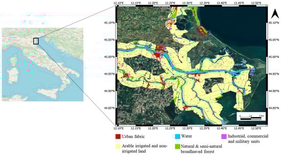
Figure 1. The area of interest (AoI) and the representation of the classes of objects present in the scene. The classes are imported from the Natura 2000 (N2K) dataset [23].

The identification of man-made objects is challenging and makes the urban classification more complex, in contrast to other classes, such as water or vegetation. Indeed, there are several categories of single and or multistorey buildings, various rooftop materials, the occurring interaction with surrounding vegetation, and the effects of look direction during data collection. To assess the validity of the chosen approach, only a portion of the entire AoI is analyzed, as illustrated in Figure 2. The selected area includes various examples of urban objects, allowing the exploitation of their intrinsic scattering properties as well as the influence of the bistatic acquisition geometry during data collection [24]. From this point on, AoI refers to the one shown in Figure 2.

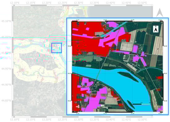
Figure 2. The visual representation of the AoI. The blue box represents the portion of the entire AoI used to assess and validate the approach. Only the classes that refer to urban objects are isolated from the entire dataset of N2K. The red zones represent the urban area, the purple zones depict industrial, commercial, and military units, while the blue zones represent the water of the River Po. (The legend is in meter scale. The legend ranges from 0 to 500 m).

To train the machine learning model, the truth data were extracted from the available data of CSLG-LC100, obtained from the open dataset available on N2K [23]. In particular, the raster data related to the AoI were imported into QGIS [25], and only those relating to the urban classes were isolated. The raster data were then exported and annotated via SeNtinel Applications Platform (SNAP) [26] on the original images to constitute the Ground Truth, which is also essential for proceeding with the evaluation of the model’s performance. The man-made objects identification and the Ground Truth are shown in the right part of Figure 3.

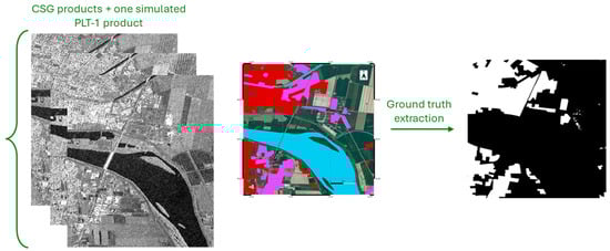
Figure 3. (Left) Selected CSG products acquiring the AoI; (Right) identification and extraction of the urban object class from the N2K site (red zones represent the urban area, the purple zones depict industrial, commercial, and military units) and Ground Truth, in which each pixel is annotated according to the object class to which they belong.

The Ground Truth extracted from the N2K dataset could be used to train a classification algorithm. However, these original annotations resulted in poor model performance. This is primarily due to the limitations of the classification map provided by CSLG-LC100 [21,22], which often includes misclassified or unclassified buildings and contains both incomplete and imprecise annotations within the area of interest, where the imprecise annotations are those in which the mask covers not only the building but also surrounding classes (e.g., vegetation, street). Therefore, a manual correction is performed before proceeding to the dataset construction. First, the buildings unidentified in the classification map were identified and manually annotated. Then, existing masks were modified to create new and more truthful annotations, enabling the model to be trained more robustly and effectively.

To highlight the differences from the original annotations, Figure 4a displays a part of the area of interest as captured by Google Earth, where man-made objects are clearly visible. Figure 4b shows the original annotations obtained from the N2K dataset, which are imprecise and inaccurate. Notably, the two central buildings in the scene remain unclassified from the original annotation, while existing annotations group multiple classes under the same mask. Figure 4c presents the manual annotations, where existing masks are refined, and new masks are added. From this point forward, the term Ground Truth will refer exclusively to these manually corrected annotations.

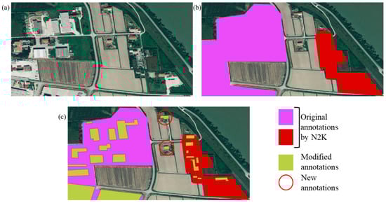
Figure 4. Example of corrected annotation on a zoom view of the AoI: (a) Google Earth image; (b) annotation taken from N2K dataset; (c) example of manual and new annotations.

Finally, to highlight the differences, Figure 5 shows the updated Ground Truth compared with the original one.

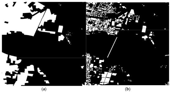
Figure 5. Presentation of the binary Ground Truth image used for training the model: (a) original Ground Truth extracted from the N2K dataset; (b) new manually corrected Ground Truth.

2.2. Monostatic–Bistatic Data Combination and Processed SAR Images

The aim of this study is to define a classifier able to process monostatic and bistatic SAR images, thus contributing as an additional information layer to the systems already used to produce the CGLS data. Within the scenario envisaged by the PLT-1 mission [11], considering that the CSG transmitter is assumed to work in Stripmap acquisition mode [14,27], the monostatic image, over the area of interest, will be available either in single polarization (HH or VV) or in dual polarization (HH and HV or VV and VH). Moreover, considering that PLT-1 receives in vertical polarization only [16], there are basically two possibilities to merge the information coming from the two platforms:

• If CSG works in a single polarization, only two images can be generated in a single-pass fashion by CSG and PLT-1. The first is related to CSG acquisition, and the second refers to PLT-1 bistatic acquisition. Hence, depending on the current transmitted and received polarization adopted by the transmitter, the following couples can be obtained: (HH_|CSG, HV_|PLT-1), (HV_|CSG, HV_|PLT-1), (VV_|CSG, VV_|PLT-1), and (VH_|CSG, VV_|PLT-1).
• If CSG works in a dual-polarization mode, three images can be acquired in a single-pass fashion. The first two images come from CSG, the latter one comes from the PLT-1 bistatic acquisition. Even in this case, different possibilities exist, namely (HH_|CSG, HV_|CSG, HV_|PLT-1) and (VV_|CSG, VH_|CSG, VV_|PLT-1).

However, due to the unavailability of the PLT-1 products at the current stage, the bistatic image is replaced in this work by a further CSG monostatic acquisition collected over the same area with a short temporal lag (days) and from a significantly different looking angle. This substitution introduces additional geometric diversity (incidence angle) useful for data-driven classification, but it is not equivalent to a true bistatic acquisition, which may involve different scattering mechanisms and calibration constraints [28,29]. In this work, the monostatic–bistatic proxy is generated at the image level from backscatter intensity channels. Therefore, the full Sinclair scattering matrix is not modelled, and cross-correlation terms between acquisitions are not exploited. The expected variations in scattering and geometric effects, even though different from an actual bistatic acquisition, are expected to introduce a sufficient diversity among the images to emulate monostatic–bistatic imagery. Processed products are listed in Table 1.

Table 1. Specifications of the COSMO-SkyMed Second Generation (CSG) products used for the simulation.

Platform	Acquisition Date	Pass Direction	Look Side	Incidence Angle	Polarization
CSG1	15 May 2023	Descending	Right	49°	HH-HV
CSG2	27 April 2023	Descending	Right	33°	HV

In particular, the first product was acquired on 15 May 2023 and is available in dual-polarization HH-HV, with an incidence angle of 49°. The second product was acquired on 27 April 2023, with polarization HV and an incidence angle of 33°. These products were properly pre-processed before entering the classification algorithm. Specifically, the following preprocessing steps have been applied using SNAP tools:

• Speckle filtering;
• Terrain correction;
• Linear to decibel (dB) conversion.

During the pre-processing steps, radiometric calibration is not applied. This is because the CSG Stripmap products used in this analysis are already radiometrically calibrated [30].

SNAP’s speckle filtering toolbox offers several options for speckle removal, e.g., Lee Sigma, Frost, Boxcar, and is worth elaborating further on the selection process for the speckle filter. Extensive investigations were conducted to assess various filters available in the SNAP Speckle Filter toolbox, aiming at identifying the most effective method for detecting and distinguishing different features within the images. Particularly, significant attention was given to evaluating the outcomes yielded by the Lee-Sigma speckle filter and the Refined-Lee speckle filter. Table 2 shows a comparison between the Lee-Sigma speckle filter and the Refined-Lee speckle filter in terms of scattering coefficient in two different polarizations.

Table 2. The comparison of minimum, mean, and maximum of the backscatter coefficient σ° (in dB) for the two CSG polarizations (HH and HV) under different speckle-filtering settings (no filter, Lee-Sigma, Refined-Lee). Speckle filtering was applied to the full scene in SNAP, and the statistics were computed after cropping to the AoI, on the resulting σ° (dB) images.

Methodology	${\mathit{\sigma }}_{\mathit{H}\mathit{V}}^0$ (dB)			${\mathit{\sigma }}_{\mathit{H}\mathit{H}}^0$ (dB)
	Min	Mean	Max	Min	Mean	Max
No speckle filter	−34.29	−23.30	−7.31	−48.70	−30.96	−13.22
Lee-Sigma	−18.54	−12.94	−7.33	−27.547	−20.53	−13.51
Refined-Lee	−19.11	−13.16	−7.22	−28.51	−20.92	−13.33

Following the speckle removal, the co-registration process was performed through SNAP’s co-registration toolbox, using the second product of Table 1 as the master image. The reported statistics values are computed over the AoI on σ° (dB) images and are intended as descriptive indicators of how the different speckle filters affect the overall backscatter distribution, not as classification performance metrics.

2.3. XGBoost Application

XGBoost is a state-of-the-art supervised classification algorithm [18] belonging to the family of gradient boosting methods. It builds an ensemble of decision trees in a sequential manner, where each new tree is trained to correct the residual errors of the previously built ensemble. This strategy allows the model to progressively refine its predictions and achieve higher accuracy and generalization performance compared to classical approaches [19,20].

One of the main advantages of XGBoost lies in its ability to combine robustness with efficiency. In this work, the classification task is point-wise, meaning that each pixel is independently assigned to a class based on its feature vector, and only a limited number of SAR images are available for training. Under these conditions, XGBoost is particularly suitable, as it can be effectively trained on relatively small datasets while maintaining strong generalization capabilities. Conversely, more complex neural network architectures would require substantially larger and more diverse training datasets, offering limited benefits in terms of classification accuracy for this specific problem. As a result, XGBoost can capture more complex and non-linear relationships while mitigating the risk of overfitting. Moreover, XGBoost is designed for scalability and computational efficiency, enabling fast training even on large datasets. Its flexibility also allows the fine-tuning of numerous hyperparameters, giving the user direct control over the trade-off between model complexity and generalization. The algorithm expects as input a structured dataset in tabular form, where each sample is described by a set of features. A feature in this context is a numerical descriptor that encodes some property of the data, such as scattering intensity, polarimetric indicators, or spatial characteristics extracted from SAR imagery and presented next in the study. When organized for training, the dataset is represented as a matrix of dimensions K × M, where K is the number of pixels and M is the number of features. Each row corresponds to a single pixel, and each column corresponds to one of the extracted features. This data organization matches XGBoost’s requirements [19], as the model is explicitly designed to operate on feature matrices. By leveraging this structure, the algorithm can learn decision rules that maximize separation between classes while exploiting its inherent advantages, such as regularization, efficient tree boosting, and advanced handling of class imbalance, to outperform more conventional supervised classification methods.

2.4. Feature Extraction and Dataset Creation

Particular attention is given to the creation of the dataset used to train the algorithm. The XGBoost algorithm was trained on a total of 48 features. The choice of these features was driven by the need to capture the different aspects that can discriminate man-made objects from other land cover types. Specifically, the adopted set of features includes not only scattering intensity but also spatial and polarimetric properties. The complete list of extracted features is provided in Table 3.

Table 3. The composition of the dataset in terms of the number and type of features. The symbol # indicates the number of the extracted features.

Features	Type	#	Explanation
Original products	SAR monostatic–bistatic intensity	3	Original SAR products in HH, HV, HV polarization
Cloude–Pottier	Polarimetric	3	Output of the Cloude–Pottier decomposition
Freeman–Durden	Polarimetric	3	Output of the Freeman–Durden decomposition
Gabor Filter	Spatial and Textural	12	Four contributions for each original image
Stationary Wavelet Transform	Frequency	12	Four contributions for each original image (LL, LH, HL, HH)
Laplacian Filter	Spatial	3	One for each original image
Sobel Filter	Spatial	6	Two for each original image. One in the x-direction and one in the y-direction
Mean and Standard Deviation	Statistical	6	One for each original image

Starting from the scattering coefficient, different σ⁰ values lead to different pixel values in the image, so the first three features are related to SAR image intensity. However, before proceeding with the feature extraction, it is important to perform image normalization. For XGBoost, normalization is not strictly needed due to the nature of decision trees. However, if the extracted features have very different scales of variation, the tree construction process could favour the feature with greater variations, especially in the first iterations. Therefore, in general, normalizing the features helps to improve the stability, convergence, and overall performance of the model. Different normalization approaches have been explored, comparing an approach without normalization, one with static (i.e., identify the absolute minimum and maximum in the dataset and normalize all features against these), and another with dynamic normalization (i.e., identify the minimum and maximum for every single feature and normalize it with respect to its maximum and minimum). Considering that each pixel of the image represents the intensity captured by the SAR, to preserve this physical information, a dynamic normalization was chosen. The normalization model is defined in Equation (1):

$$X_{norm}=a+\left({\displaystyle \frac{X-\min \left(X\right)}{\max \left(X\right)-\min \left(X\right)}}\right)\left(b-a\right),$$

(1)

where $X$ represents the value of a pixel to be normalized, $\max \left(X\right)$ and $\min \left(X\right)$ denote the maximum and minimum values of the histogram of the given image, respectively. The parameters $a$ and $b$ define the range for normalization, in this case [−1, 1]. After normalization, the histograms of the three original products are constrained within the specified range. The other types of features are fully described in the following sections. In accord with the ML model, before model training, the constructed dataset is divided once into training and test subsets using a spatially coherent hold-out region. The test subset (20%) is kept fixed for all experiments to provide an independent benchmark.

2.4.1. Cloude–Pottier Decomposition

Cloude–Pottier polarimetric decomposition is a technique used in the processing of polarimetric Synthetic Aperture Radar data. This methodology makes it possible to analyze the electromagnetic behaviour of land surfaces and interpret the physical properties of the terrain based on the radar response [31,32]. In general, the decomposition is based on a complete covariance or coherence matrix analysis. However, considering that from the CSG acquisitions, the available data are only in two distinct polarizations, HH and HV, and given the lack of a co-polarized VV component, Cloude–Pottier decomposition is modified for dual-polarization SAR applications. Following the methods proposed in [31], the modified covariance matrix to perform the polarimetric decomposition is expressed in Equation (2).

$$⟨T_{CP}⟩={\displaystyle \frac{1}{2}}\left[\begin{array}{ccc}{\left|S_{HH}+S_{HV}\right|}^2& \left(S_{HH}+S_{HV}\right){\left(S_{HH}-S_{HV}\right)}^{*}& \left(S_{HH}+S_{HV}\right)S_{HV}^{*}\\ {\left(S_{HH}+S_{HV}\right)}^{*}\left(S_{HH}-S_{HV}\right)& {\left|S_{HH}-S_{HV}\right|}^2& \left(S_{HH}-S_{HV}\right)S_{HV}^{*}\\ {S_{HV}\left(S_{HH}+S_{HV}\right)}^{*}& {S_{HV}\left(S_{HH}-S_{HV}\right)}^{*}& {\left|S_{HV}\right|}^2\end{array}\right],$$

(2)

where * denotes the complex conjugate. $S_{ij}$ is the complex signal of the SAR data, computed taking into account the in-phase component, the real part of the radar signal, and the quadrature component, which represents the imaginary part of the received radar signal. It is demonstrated that HH and HV data can only partially extract low, medium, and high entropy scattering mechanisms due to the lack of co-polarization VV [31]. However, in this context, the purpose is not to construct a detailed H-α plane, but to use the decomposition output (H, α, and A) as additional features for training the model. For this reason, these three outputs will have the same dimension as the original products and can be inserted into the dataset to constitute three additional features.

2.4.2. Freeman–Durden Decomposition

Freeman–Durden decomposition is a method used to analyze and interpret polarimetric SAR images to identify and separate different mechanisms of radar signal dispersion. The main objective is to decompose the polarimetric behaviour of the radar signal into three distinct physical scattering mechanisms [33,34], namely double-bounce, volumetric, and surface scattering. Decomposition requires full SAR polarimetric (quad-pol) images with three main channels: two in co-polarization (i.e., HH and VV) and at least one in cross-polarization (i.e., HV). Despite its wide use, the Freeman–Durden decomposition has limitations that must be considered in this work. Indeed, the method assumes that volumetric scattering is homogeneous and isotropic, which may not always be true, especially in these complex environments that include different types of targets. On the other hand, in reality, multiple scattering mechanisms may coexist in the same pixel (e.g., buildings with surrounding vegetation), leading to misclassification errors. In this study, the biggest limitation concerns data availability. The decomposition requires full polarimetric SAR data (HH, HV, and VV), which are not available in this analysis. To overcome this limitation, a modified decomposition is proposed, which uses the dual-pol data from CSG and the single-pol data acquired from PLT-1. The approach is to construct the Freeman–Durden coherence matrix, $T_{FD}$, using these three sources of information, rather than following its standard definition [34]. The modified $T_{FD}$ used for the Freeman–Durden decomposition is expressed in Equation (3):

$$⟨T_{FD}⟩=\left[\begin{array}{ccc}{\left|S_{HH}\right|}^2& S_{HH}{S_{HV}}^{*}& 0\\ {S_{HH}}^{*}{S}_{HV}& {\left|S_{HV}\right|}^2& 0\\ 0& 0& {\left|S_{HV\_PLT}\right|}^2\end{array}\right],$$

(3)

where the notation is the same used for the Cloude–Pottier decomposition, while $S_{ij\_PLT}$ is the contribution of the bistatic acquisition performed by PLT-1. The modified Freeman–Durden descriptor is adopted here as a physically informed feature extractor under the constraint of limited polarimetric availability (i.e., the lack of full quad-pol measurements). Therefore, its design is driven by the available polarization/geometry information while preserving the interpretability of the three canonical scattering contributions (surface, volume, and double bounce). It is important to highlight that, in this context, the terms representing the correlation between the monostatic acquisition of CSG and the bistatic acquisition of PLT-1 are set to zero, deviating from the standard definition of the covariance matrix. This adjustment is made because, considering the long-baseline configuration, the backscatter and the phase contributions of PLT-1 are decorrelated with respect to the ones of CSG. The same is true for repeat-pass CSG data collected with extremely different-looking angles. Following [34], a function in a Python environment was initialized to compute the covariance matrix $T_{FD}$ for each pixel and calculate its eigenvalues. It is important to emphasize that, in a strict sense, the eigenvalues, ordered in ascending order, enable differentiation between the various scattering contributions. In this context, using a different notation could be misleading, so the strict notation of the Freeman–Durden decomposition that associates the maximum eigenvalue with the volumetric scattering contribution, the minimum eigenvalue with the surface scattering contribution, and the double-bounce contribution as the difference between the first and minimum eigenvalues is maintained. The output of this function consists of three images, each emphasizing different scattering contributions. These images will have the same dimensions as the input image, allowing them to be added to the dataset as additional features for model training. An example of the output of the Freeman–Durden decomposition is shown in Figure 6, where the different scattering contributions were computed following the logic outlined above.

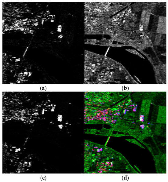
Figure 6. The output of the Freeman–Durden decomposition on the AoI: (a) double-bounce scattering; (b) surface scattering; (c) volume scattering; (d) the false colour RGB image created using R: double-bounce, G: surface scattering, and B: volume scattering as the association of the channels.

2.4.3. Gabor Features Extraction

The Gabor filter is a linear filter mostly employed in edge detection, surface evaluation, feature extraction, object recognition, and in many other applications [35,36,37]. According to [35], the filter has a real and an imaginary component, and the function used in this study is expressed in Equation (4):

$$G\left(x,y,\sigma , \theta , \lambda , \gamma , \phi \right)=\exp \left[-{\displaystyle \frac{x^2+{\gamma }^2{y}^2}{{2\sigma }^2}}\right]\exp \left[i\left({\displaystyle \frac{2\pi x}{\lambda }}+\phi \right)\right],$$

(4)

where ($x,y$) defines the kernel size, $\sigma$ is the standard deviation, $\lambda$ denotes the wavelength, $\gamma$ the aspect ratio, $\phi$ the phase offset, and $\theta$ is the orientation that defines the direction in which the filter is applied (e.g., with $\theta$ = $\pi$ the filter extracts the vertical features). In this context, a 2D Gabor filter is utilized to enhance dataset characterization and to extract spatial and textural information from the original SAR product. Specifically, the Gabor filter was initialized with the following parameters: kernel size = 20, $\gamma$ = 0.5, $\lambda$ = $\pi$/2, $\theta$ = [0, $\pi$/2], $\sigma$ = [5, 10]. In the discrete image domain, the wavelength $\lambda$ controls the central spatial frequency of the band-pass response, while $\theta$ controls the orientation of maximum sensitivity. The adopted orthogonal directions ($\theta$ = 0 and $\pi$/2) are intended to capture dominant rectilinear urban patterns at two spatial scales; it is applied independently to each acquisition (HH 49°, HV 49°, HV 33°) to exploit geometry-dependent variations in the resulting texture responses. With this set of values, applying the Gabor filter generates 4 images, one for each input image and with its dimensions. Each of these images will contribute to the dataset, resulting in a total of 12 features. Figure 7 shows an example of the application of the Gabor filter to the first product listed in Table 1.

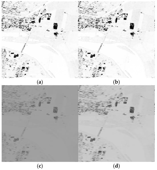
Figure 7. Output of the Gabor filtering process on AoI with a different set of parameters. (a) $\sigma =5$, $\theta =0°$; (b) $\sigma =10$, $\theta =0°$; (c) $\sigma =5$, $\theta =90°$; (d) $\sigma =10$, $\theta =90°$.

2.4.4. Stationary Wavelet Transform

Wavelet Transform (WT) is a widely used tool in computational harmonic analysis, known for its ability to provide localization in both the spatial and frequency domains. A key feature of WT is its capacity for multiresolution analysis, enabling efficient performance in applications such as data compression and denoising. Moreover, WT is excellent in highlighting local changes in the image, such as rapid intensity transitions, i.e., edges, anomalies, or rare details [38,39]. Within this framework, the Stationary Wavelet Transform (SWT) is specifically chosen to extract spatial and frequency features from the original products. With respect to WT, SWT does not reduce the size of coefficients during the extraction. This preserves spatial information and facilitates the reuse of coefficients to extract detailed features without loss of data. This is essential in dataset construction, as it preserves the size of the original images. In this study, the original products coming from CSG and PLT-1 are analyzed at different scale levels to extract texture information useful in classification and pattern recognition. SWT decomposes the three images into a series of layers, each representing image features at different frequency scales. In particular, each original image is decomposed into four different layers: low–low frequency (LLF), low–high frequency (LHF), high–low frequency (HLF), and high–high frequency (HHF). This decomposition makes it possible to identify fine high-frequency details such as edges and contours, as well as global low-frequency structures such as general shapes or textures. In this framework, SWT is applied to extract multiscale features that highlight edges (e.g., perimeters of buildings or streets) and textures (to distinguish water, vegetation, and urban areas). The extracted 12 coefficients and different layers, 4 for each original image, are inserted within the dataset and will correspond to additional features useful to training the XGBoost model. The example of the four contributions, extracted from the first product listed in Table 1, is depicted in Figure 8.

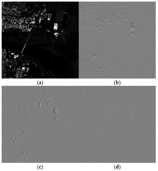
Figure 8. Output of application of SWT on AoI: (a) LLF; (b) LHF; (c) HLF; (d) HHF.

2.4.5. Sobel and Laplacian Filter

In addition to the Gabor filter, to extract edge and spatial features from the SAR products, Sobel and Laplacian filters are also used. Sobel and Laplacian edge detection are popular techniques used in image processing and computer vision for detecting edges in an image. The kernel size for Laplacian and Sobel filters is set in accordance with [40]. The Sobel operator uses two 3 × 3 convolution kernels, one for detecting changes in the x-direction and one for detecting changes in the y-direction. These kernels are used to compute the gradient of the image intensity at each point, which helps in detecting the edges. This strategy allows two features to be extracted from each SAR original product, one in the x-direction and one in the y-direction, and it is conducted on a total of six features. Regarding the Laplacian operator, it is applied, with the same logic used for the Sobel filter, at each SAR original product, leading to three additional features useful to build the dataset and to train the model. The example of the three contributions extracted from the first product listed in Table 1 is shown in Figure 9.

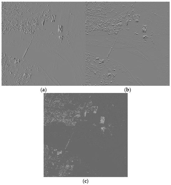
Figure 9. The output of the application of the Sobel and Laplacian filters on the AoI: (a) Sobel in x-direction; (b) Sobel in y-direction; (c) Laplacian filtering.

2.4.6. Mean and Standard Deviation

The last features inserted in the dataset are mean and standard deviation, which belong to the space of statistical features as they describe local or global statistics of the image. In this context, mean and standard deviation are applied locally by defining a kernel size of 5 × 5 that creates a local window running over the image. This helps describe local features of the image, such as textures or intensity variations. The mean and standard deviation are computed with Equations (5) and (6), respectively:

$$\mu ={\displaystyle \frac{1}{N}}\sum _{i=1}^N{I}_i,$$

(5)

$$\sigma =\sqrt{{\displaystyle \frac{1}{N}}\sum _{i=1}^N{\left(I_i-\mu \right)}^2},$$

(6)

where $N$ is the total number of pixels, and $I_i$ represents the intensity value of the i-th pixel.

3. Results

This section presents the evaluation strategy adopted to assess the classification model’s performance. It is important to underline that the accuracy associated with the CSLG-LC100 product refers to absolute classification accuracy and can be interpreted as the probability that a given pixel is correctly classified among different classes. The target accuracy of the CSLG-LC100 product is approximately 80%, and this value results from the integration of SAR data, PROBA-V optical data, and UAV data, while the estimation of the overall accuracy is carried out through in situ verification. However, at this stage of the analysis, it is not possible to estimate absolute accuracy using a single metric due to issues that will be discussed later in this section. Therefore, the accuracy of the model is evaluated through three standard metrics: Precision, Recall, and F1 score. These metrics assess the model’s ability to predict target classes by comparing its predictions with the ground truth (provided as input during training). The inability to define absolute accuracy comes from the nature of the classification task and the model itself. The model output will be a binary image where each pixel is classified as either urban or non-urban, and relying on a single score to calculate absolute accuracy is misleading. Moreover, the Ground Truth in Figure 5 shows that the number of non-urban pixels significantly exceeds that of urban pixels. This class imbalance could result in a high accuracy value, which is, again, not correct in an absolute sense. For example, the model might correctly classify most non-urban pixels while failing to accurately predict urban pixels, and this would result in a high overall accuracy value that fails to reflect the model’s inadequate performance on the minority class. Precision and Recall are important measures in machine learning that assess the performance of a model [41]. Precision evaluates the correctness of positive predictions, while Recall determines how well the model recognizes all pertinent instances [42]. Mathematically, Precision and Recall can be expressed by Equations (7) and (8), respectively:

$$Precision={\displaystyle \frac{TP}{TP+FP}},$$

(7)

$$Recall={\displaystyle \frac{TP}{TP+FN}},$$

(8)

where $TP$ marks the true positives, $FP$ marks the false positive and $FN$ marks the false negatives. Which of these metrics to maximize depends on the task. As of today, the goal is to achieve the highest possible values for both, and for this reason, the F1 score is used. It is the harmonic mean of the Precision and Recall and is expressed in Equation (9).

$$F1 score=2\times {\displaystyle \frac{Precision\times Recall}{Precision+Recall}}.$$

(9)

In general, a good F1 score indicates a good balance between Precision and Recall values.

To achieve optimal model performance, several factors must still be addressed. On one hand, the imbalance between the non-urban and urban classes presents a significant challenge that must be managed. On the other hand, fine-tuning the hyperparameters of the model can help maximize performance metrics.

3.1. Class Imbalance Management

Class imbalance is a common challenge in machine learning. Various techniques have been developed to address this issue, primarily by either increasing the number of minority-class samples (over-sampling) or reducing the number of majority-class samples (under-sampling). In this work, we tested and compared the effectiveness of the Synthetic Minority Over-sampling Technique (SMOTE) [43] with the use of the scale_pos_weight parameter, an XGBoost hyperparameter specifically designed to handle imbalanced classification problems by adjusting the model’s sensitivity to different classes.

SMOTE is a technique that uses an over-sampling approach in which the minority class is over-sampled by creating “synthetic” examples. This technique generates synthetic examples in a less application-specific manner by operating in feature space [43]. The minority class is oversampled by creating synthetic instances along the line segments connecting each sample of the minority class with one or more of its k nearest neighbours. The specific neighbours used are randomly chosen from the k nearest ones, based on the desired oversampling rate. This approach helps the classifier learn broader and more generalized decision boundaries, rather than narrow and overly specific ones. Consequently, the representation of the minority class is enhanced, preventing it from being overshadowed by the prevalence of the majority class and improving the generalization performance of decision trees. However, while the SMOTE provides significant advantages for handling unbalanced datasets, it increases computational complexity as the model must process a larger volume of data during training, alters the original non-uniform data distribution, potentially reducing its fidelity to the actual distribution, and can lead to a higher risk of overfitting.

For this reason, the use of scale_pos_weight has been evaluated in parallel with the SMOTE. Scale_pos_weight is a hyperparameter of the model that controls the balance of positive and negative weights [20,44]. By default, the scale_pos_weight hyperparameter is set to the value of 1.0 and has the effect of weighing the balance of positive examples, relative to negative examples, when boosting decision trees. XGBoost is trained to minimize a loss function, and the gradient is used as the basis for fitting subsequent trees added to boost or correct errors made by the existing state of the ensemble of decision trees. The scale_pos_weight value is used to scale the gradient for the positive class. This has the effect of scaling errors made by the model during training on the positive class and encourages the model to over-correct them [44]. This encourages the model to achieve better performance when making predictions on the positive class. However, if it is pushed too far, it can lead the model to overfit the positive class, at the expense of performing worse on the negative class or both classes. The results achieved by the SMOTE and the scale_pos_weight hyperparameter are compared on the AoI, in which the ratio of the majority class (negative) to the minority class (positive) is approximately 7:1. SMOTE allows one to set the sampling_strategy parameter, which specifies the desired ratio between the minority and majority classes. A sampling_strategy = 1 indicates a perfect balance, meaning the number of samples in the minority class will be equal to those in the majority class. In contrast, a sampling_strategy = 0 means no changes will be made to the original class distribution. Figure 10 shows that the two techniques produce equivalent results. For both approaches, the F1 score increases as the ratio of positive to negative samples rises, either through a higher percentage of synthetic samples with SMOTE or by increasing the scale_pos_weight parameter. It is worth noting that Precision and Recall trends are similar for both methods but exhibit inverse behaviour, consistent with the definitions provided in Equations (7) and (8). Using the SMOTE, the highest F1 score is achieved with a sampling_strategy of 0.25, while the optimal F1 score using the scale_pos_weight parameter is reached around a value of 1.9. It is observable that excessively high values of scale_pos_weight or sampling_strategy lead to overfitting, resulting in a decline in the model’s performance.

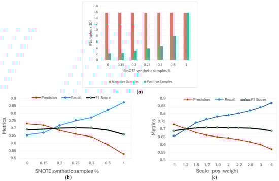
Figure 10. Comparison between SMOTE and scale_pos_weight use: (a) histogram of negative and positive class samples (the symbol # indicate the number); (b,c) comparison of Precision, Recall, and F1 score metrics under varying synthetic data generation and scale_pos_weight.

Table 4 provides a comprehensive comparison of Precision, Recall, and F1 values for both methods. Since the two methods appear equivalent, adjusting the XGBoost gradient using the scale_pos_weight hyperparameter, rather than generating synthetic data with the SMOTE, seems to be a better approach. For this reason, only the scale_pos_weight will be adjusted in the continuation of the analysis, in line with the previous evaluation.

Table 4. Metrics evaluation with different values of synthetic samples and scale_pos_weight.

% Synthetic Samples	Precision	Recall	F1 Score
Original (=0)	0.728	0.655	0.690
0.15	0.718	0.669	0.693
0.20	0.685	0.718	0.701
0.25	0.660	0.749	0.702
0.30	0.642	0.771	0.701
0.50	0.591	0.822	0.688
1.00	0.526	0.875	0.657
Scale_pos_weight
Default (=1.0)	0.728	0.655	0.690
1.5	0.676	0.740	0.707
1.7	0.662	0.762	0.708
1.9	0.648	0.782	0.709
2.0	0.642	0.789	0.708
2.2	0.632	0.802	0.707
2.5	0.617	0.820	0.705
3.0	0.599	0.841	0.700
4.0	0.570	0.870	0.689

3.2. Hyperparameter Tuning

Preliminary tests comparing XGBoost with a Random Forest baseline have been performed in the early stage of the study. XGBoost provided consistently higher performance in general, and so, it has been selected for subsequent experiments. XGBoost offers several hyperparameters that directly interact with the model’s objective function. Unlike the parameters learned during training, hyperparameters are predefined and play a key role in shaping the learning process. One common approach to finding the best hyperparameters is through methods like grid search analysis [45], where a parameter’s grid is defined, and various combinations of specified parameter values are evaluated against a specified evaluation metric, in this case, the F1 score [46]. This grid establishes the potential values for each hyperparameter. Once a grid with possible values for each hyperparameter is defined, the model is trained, and its performance is evaluated for each combination using k-fold cross-validation as the validation technique. Finally, a selection of the set of hyperparameters that yields the best performance is carried out. Although this approach is straightforward to implement and use, it comes with high computational costs, particularly when searching for the optimal combination among a large set of hyperparameters and/or possible values. Before training the model, the data are divided into the test data and the training data. Following [47], in this analysis, the training data are further divided into two parts, training data and validation data, following an iterative process that splits the data into k partitions. Each iteration keeps one partition for testing and the remaining k − 1 partitions for training the model. The next iteration sets the next partition as test data and the remaining k − 1 as train data, and so on. In each iteration, the process records the performance of the model, also giving the average of all the performances at the end. This process makes grid search analysis a highly time-consuming technique. In particular, the higher the k parameter in k-fold cross-validation, the longer it takes to determine the optimal combination of hyperparameters. For this reason, k = 3 was chosen at this stage, providing a balance between ensuring a sufficiently robust validation while keeping the model training time manageable. Table 5 shows the XGBoost hyperparameters, on which k-fold cross-validation is conducted with their simple explanation and default value (if not set) [48,49].

Table 5. Ranges of hyperparameter values to conduct the grid search analysis.

Hyperparameter	Default Value	Value
Max_depth	6	9, 10
Min_child_weight	1	3.2, 3.4, 3.6
Scale_pos_weight	1	1.9, 2.5
Learning_rate	0.3	0.1, 0.15, 0.2, 0.8
${\alpha }_{L1}$	0	0.8, 1, 1.2
${\lambda }_{L2}$	1	0.1, 0.5, 1

The influence of various hyperparameters on the model’s performance, measured through the F1 score, is explored by varying learning_rate against different parameters such as max_depth, ${\alpha }_{L1}$, and ${\lambda }_{L2}$. However, since the differences among the results are generally small, only one representative example is reported in Figure 11, where learning_rate is analyzed in combination with the min_child_weight. This pair of hyperparameters is chosen as an illustrative case.

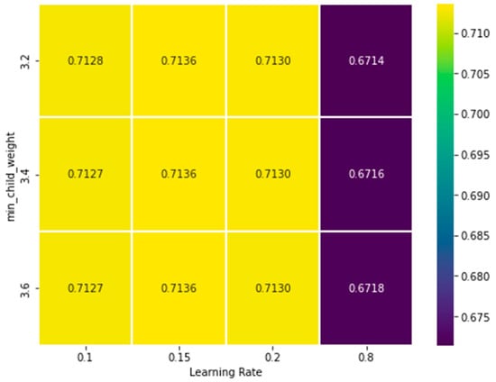
Figure 11. The heatmap of variation in learning rate and min_child_weight to reach the best F1 score. Each cell represents a single F1 score value associated with a specific combination of the two chosen hyperparameters.

As expected, learning_rate controls how fast the model adapts to the training data, while min_child_weight regulates the minimum number of samples required for a node split, effectively balancing model complexity and generalization.

The colour intensity in each cell of the heatmap represents the F1 score value for the corresponding parameter combination. For each pair of varying hyperparameters, the different values of the remaining fixed ones (e.g., scale_pos_weight or ${\alpha }_{L1}$) is also considered.

Since it is not feasible to explore all possible hyperparameter combinations (433 × 3) simultaneously, the F1 score associated with a given point in the heatmap is computed as the average across the different settings of the other parameters. For instance, for a combination of learning_rate = 0.1 and min_child_weight = 3.2, multiple F1 scores may arise depending on the values of scale_pos_weight. By averaging the different F1 scores, a single representative value is obtained, summarizing the performance of that combination.

The heatmap shown in Figure 11 illustrates that the best F1 scores are obtained when learning_rate is set between 0.1 and 0.2, combined with min_child_weight around 3.2. For example, increasing learning_rate from 0.1 to 0.8, while keeping min_child_weight fixed, reduces the model stability and leads to a noticeable decrease in F1 score. Similarly, setting min_child_weight above 3.6 constrains tree growth too strongly, preventing the model from capturing smaller urban objects and leading to more false negatives.

Overall, this pairwise analysis was conducted for all the hyperparameters listed above, with learning_rate compared in turn with max_depth, ${\alpha }_{L1}$, and ${\lambda }_{L2}$, while keeping the remaining parameters fixed. This exploration makes it possible to evaluate how different ranges influence the F1 score and mostly to identify the combination of values that maximizes this score and leads to a better model’s performance. The outcome of this process is the selection of the optimal hyperparameters used for training, which are summarized in Table 6.

Table 6. Hyperparameters chosen to train the XGBoost model.

Hyperparameter	Chosen Value
Max_depth	10
Min_child_weight	3.2
Scale_pos_weight	1.9
Learning_rate	0.15
${\alpha }_{L1}$	1
${\lambda }_{L2}$	0.1
Threshold	0.54

In machine learning models, and particularly in XGBoost, the prediction is returned in the form of a probability associated with the positive class. To convert this probability into a binary decision (class 0 or class 1), a classification threshold must be defined. By default, XGBoost uses a threshold of 0.5, which means that an observation is classified as “positive” if the predicted probability is greater than or equal to 0.5; otherwise, it is classified as “negative”. However, this threshold is not always the optimal choice, because in many applications the balance between Precision and Recall is crucial. In this context, in parallel with hyperparameter tuning, a further analysis has been conducted to optimize the classification threshold, aiming to achieve the best trade-off between these two metrics by maximizing the F1 score. Moreover, adjusting the threshold is particularly beneficial when dealing with imbalanced datasets, as it can enhance the recognition of the minority class. Threshold optimization was carried out by evaluating different threshold values and selecting the one that maximized the metric of interest, the F1 score. Specifically, Figure 12 illustrates the adopted strategy, where a variable threshold has been tested between 0 and 1, with a step size of 0.01.

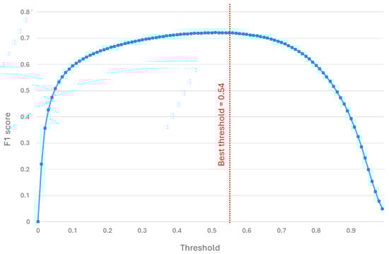
Figure 12. F1 score computed for different threshold values. The vertical red line highlighted the threshold value for the best F1 score.

The results indicate that the threshold maximizing the F1 score is close to the model’s default value, settling at 0.54. Therefore, adopting this optimized threshold enhances the balance between Precision and Recall, resulting in a more robust and better-suited model for the application context. Following the presented study, the hyperparameters chosen for training the model have been selected and are summarized in Table 6.

It is worth clarifying that the XGBoost hyperparameters reported here are not claimed to be universal. When other scenarios are selected, parameters linked to class imbalance and model complexity (e.g., scale_pos_weight, max_depth, min_child_weight, and regularization terms) should be re-optimized with the same cross-validated tuning strategy adopted in this work.

3.3. Validation and Performance Assessment

To assess the performance and accuracy of the model, the Ground Truth and the model’s predictions are compared as depicted in Figure 13. This representation provides an initial visual and qualitative feedback to the model’s ability to accurately differentiate between classes of urban and non-urban.

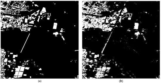
Figure 13. Qualitative representation of the final prediction outcome of the XGBoost algorithm compared with the Ground Truth used for training: (a) Ground Truth; (b) Prediction of the XGBoost model.

To evaluate the performance of the model in quantitative terms, a detailed analysis has been conducted using the confusion matrix [50], as shown in Figure 14.

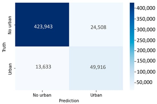
Figure 14. Confusion matrix for the final configuration (80% training, fixed 20% test).

The confusion matrix highlights that the main error mode is false positives, which is consistent with the presence of unannotated man-made targets (e.g., trellis/vehicles) discussed in Section 4. To guarantee a consistent validation strategy, the dataset was divided into two subsets, using 80% of the samples for training and the remaining 20% for testing. The 20% test set was kept fixed throughout all training configurations to provide an independent and invariant benchmark for performance evaluation and to avoid the random variability introduced by repeated re-splitting of the data. The test set corresponds to a spatially coherent portion of the AoI rather than a pixel-wise random hold-out. This is necessary to reduce the optimistic bias caused by spatial autocorrelation. Since some features use local spatial support (e.g., Gabor filter), using spatial hold-out for testing is preferred over random pixel-wise splitting [51].

The model was trained using three different portions of the available training data, corresponding to 50%, 70%, and 80% (full dataset) of the total dataset. The goal of this strategy is to evaluate both the evolution of model performance and its robustness to variations in the amount of available training data while keeping the same independent test set for validation. All training configurations used the same set of hyperparameters identified during the tuning phase and reported in Table 6. The different trained models were evaluated in terms of Precision, Recall, and F1 score. In addition to the standard metrics, the True Positive Percentage (TP%) accuracy was also computed to provide a more direct indication of the model’s ability to correctly identify the positive class (i.e., the urban objects). It is defined as the ratio between the correctly predicted positives and the total number of positive samples in the test set, and it is computed in accordance with Equation (10):

$$TP\% Accuracy={\displaystyle \frac{TP (in test set)}{AP (in test set)}},$$

(10)

The obtained results are shown and summarized in Table 7.

Table 7. Metrics and percentages of the TP accuracy for different sizes of training data.

Training Set	Precision	Recall	F1 Score	TP% Accuracy
50%	0.668	0.775	0.718	0.775
70%	0.669	0.783	0.722	0.783
80%	0.669	0.785	0.723	0.785

The results show that all metrics are stable across different training sizes, with improvements as the amount of training data increases. Specifically, the model trained with 50% of the total data achieved a Precision of 0.67, a Recall of 0.78, and an F1 score of 0.72. When the proportion of training data was increased to 70% and 80%, both Recall and F1 score slightly improved, reaching 0.785 and 0.723, respectively, for the largest training set. To quantify the contribution of the additional incidence-angle acquisition, an experiment using only the two monostatic CSG1 channels (HH 49°, HV 49°) was performed and evaluated with the same validation protocol adopted in this section. In this baseline, the feature set necessarily reduces from 48 to 31, since the modified Freeman–Durden descriptor cannot be computed and all per-image descriptors scale with the number of inputs (Gabor from 12 to 8, SWT from 12 to 8, Laplacian from 3 to 2, Sobel from 6 to 4, and mean and standard deviation from 6 to 4). Using only CSG1, the model achieves F1 = 0.670–0.675 across the three training configurations, while the full three-product configuration reaches F1 = 0.718–0.723. The gain is mainly driven by the Recall increase, indicating improved sensitivity to man-made objects when the additional viewing geometry is available. This behaviour confirms that the classifier benefits from a broader representation of the input space, leading to enhanced robustness and generalization, while maintaining stable Precision values. The results demonstrate the overall stability of the XGBoost classifier and its capacity to generalize effectively even when trained with a reduced number of samples. As expected, providing more training data leads to higher Recall and F1 score values, confirming that the model learns progressively richer class representations. The 50% and 70% training configurations are obtained by reducing the amount of training samples while keeping the same fixed test region unchanged, thus producing a robustness learning analysis under an invariant spatial benchmark.

4. Discussion

Overall, the model shows promising quantitative and qualitative results. Across the different train/test splits, metrics are stable (Precision ≈ 0.67, Recall ≈ 0.78, and F1 ≈ 0.72–0.73), while the predicted image in Figure 13 exhibits good spatial agreement with the Ground Truth. Further improvements are expected by enlarging and diversifying the dataset. Even though this type of monostatic–bistatic data is not available at the present time and systematic spaceborne bistatic benchmarks are still emerging, a direct experimental comparison with recent bistatic space-based SAR classification methods is currently not feasible; therefore, this work should be interpreted as a test of the proposed processing chain. Increasing positive examples should strengthen minority-class learning and leading into higher Precision without sacrificing Recall and so increasing the F1 score.

At present, the main limitation is the occurrence of false positives, often linked to unmodeled or unannotated man-made targets (e.g., vehicles, trellis, or highly reflective infrastructures) and to local geometrical effects. Despite this, the achieved results are already in line with the 80% requirement. In fact, the confusion-matrix analysis indicates true-positive rates around 0.78–0.83, which is consistent with the accuracy of 80% and supports the suitability of the proposed approach for downstream land-cover services.

False positives predicted by the model are affected by the presence of various man-made objects, which, for practical reasons, cannot be annotated in the Ground Truth construction phase. These man-made objects include targets like cars and trellis. The shape and material of these objects make them systematically predictable by the model, which classifies them as FP and lowers the performance of the model in terms of metrics. This is linked to the scattering behaviour exhibited by these objects when observed in a particular acquisition geometry. It is interesting to highlight some peculiar features of trellis. These objects are characterized by a repetitive shape and material; additionally, they are often far from other types of artificial targets. These peculiarities make these objects precious from a classification point of view, as shown in Figure 15.

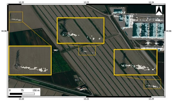
Figure 15. The superposition between the Google Earth image and the prediction image. The white pixels are associated with the true prediction by the model. The yellow box highlights the zoom-view of the target of interest.

The background in Figure 15 consists of a scene captured from Google Earth, overlaid with the model’s predictions. These predictions are represented as a binary image, with predicted positives highlighted in white pixels. The yellow boxes in Figure 15 contain zoomed-in views of specific targets within the scene. As shown, the trellis in the image is identified as a positive prediction by the model. However, within the evaluation metrics, they contribute to a decrease in the F1 score, as they are classified as false positives. This suggests that XGBoost can detect man-made objects, even those not manually annotated. Comparing the model’s predictions with the Google Earth image reveals a spatial shift between the position of the trellis and the prediction performed by the model. This shift is attributed to layover effects in the SAR image.

Analyzing the model’s predictions reveals that other false positives are often linked to moving objects, such as cars or large parking areas. These false positives are highly variable and challenging to predict accurately, as they do not follow a systematic pattern but rather depend on time and the spatial configuration of acquisitions. However, false alarms caused by moving objects can be mitigated through time-series analysis, where multiple images of the same area are captured over time to reduce this effect.

One further point that deserves consideration concerns the composition of the dataset of features. Within the set of 48 features employed for training, one should assess whether all of them contributed meaningfully to the achieved performance, or whether a significant share of the result was sustained by a smaller core subset. This analysis also contributes to the explainability of results. For this purpose, a feature importance evaluation was carried out using the internal criteria of XGBoost, i.e., gain-based ranking, aggregated across folds. The complete ranking of features by importance score was obtained, but for the sake of clarity, Table 8 reports only the top three and the bottom three features, which represent the most and least relevant contributors to model training.

Table 8. The feature importance ranking. The importance score is computed using the gain criterion in XGBoost and normalized such that the total sum equals 1, allowing a direct comparison of the relative contribution of each feature.

Feature	Importance Score
$\mathrm{Gabor} \mathrm{Filter} ($$\gamma =0.5,$ $\lambda =\pi$$/2,$ $\theta =0, \sigma$ = 10) on HV product with 33° of incidence angle	0.4538
Freeman–Durden decomposition	0.1014
$\mathrm{Gabor} \mathrm{Filter} ($$\gamma =0.5,$ $\lambda =\pi$$/2,$ $\theta =0, \sigma$ = 10) on HV product with 49° of incidence angle	0.0740
…	…
…	…
…	…
$\mathrm{Gabor} \mathrm{Filter} ($$\gamma =0.5,$ $\lambda =\pi$$/2,$ $\theta =\pi$$/2, \sigma$ = 5) on HH product with 49° of incidence angle	0.0027
Laplacian filter on HH product with 33° of incidence angle	0.0026
Laplacian filter on HV product with 49° of incidence angle	0.0026

The results clearly show that the contribution of the features is far from being uniform. The top three features alone account for about 63% of the total importance, indicating that a substantial portion of the performance is sustained by a compact subset of descriptors. This finding is physically consistent with the problem. Indeed, the Gabor filters, applied on HV polarization at different incidence angles, capture the rectilinear structures and contours typical of urban areas, while the volumetric scattering component enhances the separation between built-up and natural surfaces. Alongside this dominant core, some statistical and spatial features provide intermediate contributions, helping refine class separation, though with significantly lower weight. At the opposite end, several features contributed only marginally. In particular, the Gabor filter, applied on HH polarization, and the Laplacian filter, together account for less than 1.3% of the total importance, suggesting that their incremental value beyond the leading features is marginal. Although the presence of these characteristics does not necessarily compromise performance, their exclusion can simplify the model without a substantial decrease in accuracy. The prominence of HV 33° derived descriptors supports the interpretation that the additional geometry provides complementary information. This qualitative evidence is also confirmed by the ablation experiment reported in Section 3.3. Furthermore, when training the same pipeline using only the two CSG1 channels (HH 49°, HV 49°) and the corresponding reduced feature set (31 features), the F1 score decreases to 0.670–0.675. When the additional HV 33° acquisition is included, the F1 score increases to 0.718–0.723, mainly driven by a marked Recall gain. Overall, this indicates that the additional incidence-angle observation improves the detectability of man-made objects by providing complementary textural/scattering information.

5. Conclusions

Multi-angle repeat-pass CSG products were used in this work to support discrimination of man-made objects for LULC tasks. This strategy was adopted to approximate the benefit of combining observations acquired under different viewing geometries, emulating a bistatic scenario. Nevertheless, repeat-pass monostatic data do not capture bistatic-specific effects (e.g., possible deviations from reciprocity assumptions and geometry-dependent bistatic polarimetric or Radar Cross Section (RCS) responses). Therefore, the transferability of the learned features to monostatic–bistatic SAR must be verified using real bistatic data. The presented work is a proof of concept aimed at building and validating a complete processing chain, so that the methodology can be readily applied to real monostatic–bistatic images in the near future. Hence, a case-study validation has been carried out on a single area supported by a manually refined Ground Truth mask. In a longer-term perspective, the same framework is expected to be extended beyond the present binary task, for instance, by addressing a broader range of land-cover classes or by exploring application domains other than urban object detection. Furthermore, additional experiments are needed to assess transferability across regions with different land-cover composition and urban morphology. Future work will thus extend the validation to multiple areas and, when compatible acquisition modes are available, to publicly accessible SAR datasets in order to quantify cross-region generalization.

Reproducibility

The experiments were performed using QGIS 3.36, Maidenhead, and ESA SNAP v10.0 for SAR pre-processing. The machine configuration and software environment were as follows: OS: Windows 11, CPU: 11th Gen Intel(R) Core(TM) i7-11800H @ 2.30 GHz, RAM: 16 GB, GPU: 4 GB VRAM. Model training and feature extraction were implemented in Python 3.12.1 using XGBoost 2.0.3 and Scikit-learn 1.5.0. Key dependencies include NumPy 1.26.3, SciPy 1.11.4, Pandas 2.2.2, OpenCV 4.10.0, and rasterio 1.3.10.

References

- Copernicus Land Monitoring Service. Available online: https://land.copernicus.eu/en (accessed on 1 July 2025).
- Global Dynamic Land Cover. Available online: https://land.copernicus.eu/en/products/global-dynamic-land-cover (accessed on 1 July 2025).
- Buchhorn, M.; Smets, B.; Bertels, L.; De Roo, B.; Lesiv, M.; Tsendbazar, N.E.; Linlin, L.; Tarko, A. Copernicus Global Land Service: Land Cover 100 m: Version 3 Globe 2015–2019: Product User Manual; Zenodo: Geneve, Switzerland, 2020. [Google Scholar] [CrossRef]
- Huang, Z.; Dumitru, C.; Pan, Z.; Lei, B.; Datcu, M. Classification of Large-Scale High-Resolution SAR Images with Deep Transfer Learning. IEEE Geosci. Remote Sens. Lett. 2020, 18, 107–111. [Google Scholar] [CrossRef]
- Ahishali, M.; Kiranyaz, S.; Ince, T.; Gabbouj, M. Classification of Polarimetric SAR Images Using Compact Convolutional Neural Networks. GISci. Remote Sens. 2021, 58, 28–47. [Google Scholar] [CrossRef]
- Leinss, S.; Wicki, R.; Holenstein, S.; Baffelli, S.; Bühler, Y. Snow avalanche detection and mapping in multitemporal and multiorbital radar images from TerraSAR-X and Sentinel-1. Nat. Hazards Earth Syst. Sci. 2020, 20, 1783–1803. [Google Scholar] [CrossRef]
- Shahzad, M.; Maurer, M.; Fraundorfer, F.; Wang, Y.; Zhu, X. Buildings Detection in VHR SAR Images Using Fully Convolution Neural Networks. IEEE Trans. Geosci. Remote Sens. 2018, 57, 1100–1116. [Google Scholar] [CrossRef]
- Moccia, A.; Renga, A. Bistatic synthetic aperture radar. In Distributed Space Missions for Earth System Monitoring; Springer: New York, NY, USA, 2013; Volume 31. [Google Scholar]
- Moccia, A.; D’Errico, M. Bistatic SAR for Earth Observation; Cherniakov, M., Ed.; John Wiley & Sons Ltd.: Chichester, UK, 2008. [Google Scholar]
- Dekker, P.L.; Rott, H.; Prats-Iraola, P.; Chapron, B.; Scipal, K.; Witte, E. Harmony: An Earth Explorer 10 Mission Candidate to Observe Land, Ice, and Ocean Surface Dynamics. In Proceedings of the 2019 IEEE International Geoscience and Remote Sensing Symposium, Yokohama, Japan, 28 July–2 August 2019. [Google Scholar] [CrossRef]
- Pulcino, V.; Ansalone, L.; Longo, F.; Blasone, G.P.; Picchiani, M.; Luciani, R.; Zoffoli, S.; Tapete, D.; Virelli, M.; Rinaldi, M.; et al. PLATiNO-1 mission: A compact X-band monostatic and bistatic SAR. In Proceedings of the 75th International Astronautical Congress (IAC 2024), Milan, Italy, 14–18 October 2024. [Google Scholar]
- Gebert, N.; Dominguez, B.C.; Davidson, M.W.; Martin, M.D.; Silvestrin, P. SAOCOM-CS—A passive companion to SAOCOM for singlepass L-band SAR interferometry. In Proceedings of the 10th European Conference on Synthetic Aperture Radar, Berlin, Germany, 3–5 June 2014; pp. 1251–1254. [Google Scholar]
- Capella Space. Available online: https://www.capellaspace.com/blog/capella-space-r-d-team-demonstrates-bistatic-collect-capability (accessed on 10 January 2026).
- Agenzia Spaziale Italiana (ASI). COSMO-SkyMed Mission and Products Description. 2016. Available online: https://www.asi.it/wp-content/uploads/2019/08/COSMO-SkyMed-Mission-and-Products-Description_rev3-1.pdf (accessed on 13 March 2024).
- PLATiNO Minisatellite Platform. Available online: https://www.eoportal.org/satellite-missions/platino#references (accessed on 29 June 2025).
- Renga, A.; Gigantino, A.; Graziano, M.D.; Moccia, A.; Tebaldini, S.; Monti-Guarnieri, A.; Rocca, F.; Verde, S.; Zamparelli, V.; Mastro, P.; et al. Bistatic SAR Techniques and Products in a long baseline spaceborne scenario: Application to PLATiNO-1 mission. In Proceedings of the 15th European Conference on Synthetic Aperture Radar, Munich, Germany, 23–26 April 2024. [Google Scholar]
- Gigantino, A.; Renga, A.; Graziano, M.D.; Moccia, A.; Verde, A.; Tedesco, L.; Blasone, G.P.; Zoffoli, S.; Tapete, D.; Pulcino, V. Bistatic Observation Opportunities in PLATiNO-1 SAR Mission. In IAF Earth Observation Symposium, Held at the 75th International Astronautical Congress (IAC 2024); International Astronautical Federation (IAF): Milan, Italy, 2024; pp. 544–550. [Google Scholar] [CrossRef]
- Perissin, D.; Wang, T. Repeat-Pass SAR Interferometry with Partially Coherent Targets. IEEE Trans. Geosci. Remote Sens. 2011, 50, 271–280. [Google Scholar] [CrossRef]
- Chen, T.; Guestrin, C. XGBoost: A Scalable Tree Boosting System. In Proceedings of the 22nd ACM SIGKDD International Conference on Knowledge Discovery and Data Mining, San Francisco, CA, USA, 13–17 August 2016; pp. 785–794. [Google Scholar] [CrossRef]
- XGBoost Developers. XGBoost Documentation. Revision ae68466e. Available online: https://xgboost.readthedocs.io/en/stable/ (accessed on 5 December 2024).
- Buck, O.; Sousa, A. Copernicus Land Monitoring Service N2K User Manual 1|Page N2K Product User Manual (Version 1.0). Available online: https://land.copernicus.eu/en/products/n2k (accessed on 10 January 2026).
- European Environment Agency (EEA). Copernicus Land Monitoring Service Riparian Zones LC/LU and Change 2012–2018. Available online: https://land.copernicus.eu/en/products/riparian-zones (accessed on 10 January 2026).
- European Environment Agency (EEA). Natura 2000—Spatial Data. Available online: https://www.eea.europa.eu/data-and-maps/data/natura-14/natura-2000-spatial-data (accessed on 20 May 2025).
- Pradhan, B.; Abdullahi, S.; Seddighi, Y. Detection of urban environments using advanced land observing satellite phased array type L-band synthetic aperture radar data through different classification techniques. J. Appl. Remote Sens. 2016, 10, 036029. [Google Scholar] [CrossRef]
- QGIS Maidenhead—Version 3.36. Available online: https://www.qgis.org/ (accessed on 5 December 2024).
- European Space Agency (ESA). SNAP (Sentinel Application Platform)—Software for Processing Sentinel Data. EO Science for Society. Available online: https://eo4society.esa.int/resources/snap/ (accessed on 27 May 2024).
- European Space Agency (ESA). COSMO-SkyMed Second Generation. Earth Online. Available online: https://earth.esa.int/eogateway/missions/cosmo-skymed-second-generation (accessed on 3 September 2024).
- Krieger, G.; Moreira, A.; Fiedler, H.; Hajnsek, I.; Werner, M.; Younis, M.; Zink, M. TanDEM-X: A Satellite Formation for High-Resolution SAR Interferometry. IEEE Trans. Geosci. Remote Sens. 2007, 45, 3317–3341. [Google Scholar] [CrossRef]
- Krieger, G.; Zink, M.; Bachmann, M.; Bräutigam, B.; Schulze, D.; Martone, M.; Rizzoli, P.; Steinbrecher, U.; Antony, J.W.; De Zan, F.; et al. TanDEM-X: A Radar Interferometer with Two Formation Flying Satellites. Acta Astronaut. 2013, 89, 83–98. [Google Scholar] [CrossRef]
- Agenzia Spaziale Italiana (ASI). COSMO-SkyMed Seconda Generazione: System and Products Description; Agenzia Spaziale Italiana: Rome, Italy, 2021.
- Ji, K.; Wu, Y. Scattering Mechanism Extraction by a Modified Cloude-Pottier Decomposition for Dual Polarization SAR. Remote Sens. 2015, 7, 7447–7470. [Google Scholar] [CrossRef]
- Cloude, S.R.; Pottier, E. An entropy based classification scheme for land applications of polarimetric SAR. IEEE Trans. Geosci. Remote Sens. 1997, 35, 68–78. [Google Scholar] [CrossRef]
- Freeman, A.; Durden, S.L. A three-component scattering model for polarimetric SAR data. IEEE Trans. Geosci. Remote Sens. 1998, 36, 963–973. [Google Scholar] [CrossRef]
- Guo, S.; Li, Y.; Yin, Q.; Chen, H.; Richardson, A.; Hong, W. Applying the Freeman-Durden decomposition tocompact polarimetric SAR Interferometry. In Proceedings of the 2014 IEEE Geoscience and Remote Sensing Symposium, Quebec City, QC, Canada, 13–18 July 2014; pp. 3486–3489. [Google Scholar] [CrossRef]
- Fogel, I.; Sagi, D. Gabor filters as texture discriminator. Biol. Cybern. 1989, 61, 103–113. [Google Scholar] [CrossRef]
- Xiang, Y.; Wang, F.; Wan, L.; You, H. An Advanced Multiscale Edge Detector Based on Gabor Filters for SAR Imagery. IEEE Geosci. Remote Sens. Lett. 2017, 14, 1522–1526. [Google Scholar] [CrossRef]
- Munawar, H.S.; Aggarwal, R.; Qadir, Z.; Khan, S.I.; Kouzani, A.Z.; Mahmud, M.A.P. A Gabor Filter-Based Protocol for Automated Image-Based Building Detection. Buildings 2021, 11, 302. [Google Scholar] [CrossRef]
- Lee, G.; Gommers, R.; Waselewski, F.; Wohlfahrt, K.; O’Leary, A. PyWavelets: A Python package for wavelet analysis. J. Open Source Softw. 2019, 4, 1237. [Google Scholar] [CrossRef]
- Procházka, A.; Kukal, J.; Vyšata, O. Wavelet Transform Use for Feature Extraction and EEG Signal Segments Classification. In Proceedings of the 2008 3rd International Symposium on Communications, Control, and Signal Processing, ISCCSP 2008, Saint Julian’s, Malta, 12–14 March 2008; pp. 719–722. [Google Scholar] [CrossRef]
- Malche, T. Edge Detection in Image Processing: An Introduction. Roboflow. Available online: https://blog.roboflow.com/edge-detection/ (accessed on 5 December 2024).
- Huilgol, P. Precision and Recall in Machine Learning. Analytics Vidhya. Available online: https://www.analyticsvidhya.com/articles/precision-and-recall-in-machine-learning/#What_is_Precision? (accessed on 5 December 2024).
- Kundu, R. Precision vs. Recall: Differences, Use Cases & Evaluation. V7 Labs. Available online: https://www.v7labs.com/blog/precision-vs-recall-guide (accessed on 5 December 2024).
- Chawla, N.; Bowyer, K.; Hall, L.; Kegelmeyer, W. SMOTE: Synthetic Minority Over-sampling Technique. J. Artif. Intell. Res. (JAIR) 2002, 16, 321–357. [Google Scholar] [CrossRef]
- Brownlee, J. How to Configure XGBoost for Imbalanced Classification. Machine Learning Mastery. Available online: https://machinelearningmastery.com/xgboost-for-imbalanced-classification/ (accessed on 27 February 2025).
- Shah, R. Tune Hyperparameters with GridSearchCV. Analytics Vidhya. Available online: https://www.analyticsvidhya.com/blog/2021/06/tune-hyperparameters-with-gridsearchcv/#h-what-is-gridsearchcv (accessed on 27 February 2025).
- Hyperparameter Tuning. Algoretico. Available online: https://algoretico.it/it/magazine/tech/hyperparameter-tuning (accessed on 27 February 2025).
- Brownlee, J. A Gentle Introduction to k-Fold Cross-Validation. Machine Learning Mastery. Available online: https://machinelearningmastery.com/k-fold-cross-validation/ (accessed on 27 February 2025).
- XGBoost Developer. XGBoost Parameters. XGBoost Documentation. Available online: https://xgboost.readthedocs.io/en/stable/parameter.html (accessed on 27 February 2025).
- Jain, A. XGBoost Parameters Tuning: A Complete Guide with Python Codes. Analytics Vidhya. Available online: https://www.analyticsvidhya.com/blog/2016/03/complete-guide-parameter-tuning-xgboost-with-codes-python/ (accessed on 27 February 2025).
- Kundu, R. Confusion Matrix: How To Use It & Interpret Results [Examples]. V7 Labs. Available online: https://www.v7labs.com/blog/confusion-matrix-guide#confusion-matrix-for-binary-classes (accessed on 13 March 2024).
- Roberts, D.R.; Bahn, V.; Ciuti, S.; Boyce, M.S.; Elith, J.; Guillera-Arroita, G.; Hauenstein, S.; Lahoz-Monfort, J.J.; Schröder, B.; Thuiller, W.; et al. Cross-validation strategies for data with temporal, spatial, hierarchical, or phylogenetic structure. Ecography 2017, 40, 913–929. [Google Scholar] [CrossRef]
Disclaimer/Publisher’s Note: The statements, opinions and data contained in all publications are solely those of the individual author(s) and contributor(s) and not of MDPI and/or the editor(s). MDPI and/or the editor(s) disclaim responsibility for any injury to people or property resulting from any ideas, methods, instructions or products referred to in the content. |
© 2026 by the authors. Licensee MDPI, Basel, Switzerland. This article is an open access article distributed under the terms and conditions of the Creative Commons Attribution (CC BY) license.