Highlights
What are the main findings?
- A novel Shape-Aware Attention Network (SAANet) is proposed, establishing a unified paradigm to effectively resolve the challenges of complex stray light interference and dense overlapping trajectories.
- SAANet achieves state-of-the-art performance in challenging scenarios with intense stray light interference and dense trajectories, demonstrating superior precision with APs of 0.864 and 0.815 on benchmark datasets.
What is the implication of the main finding?
- This study provides a high-precision and robust technical solution for Space Situational Awareness (SSA), enhancing the ability to monitor and manage the increasingly crowded space environment.
Abstract
With the deployment of mega-constellations, the proliferation of on-orbit Resident Space Objects (RSOs) poses a severe challenge to Space Situational Awareness (SSA). RSOs produce elongated and stripe-like signatures in long-exposure imagery as a result of their relative orbital motion. The accurate detection of these signatures is essential for critical applications like satellite navigation and space debris monitoring. However, on-orbit detection faces two challenges: the obscuration of dim RSOs by complex stray light interference, and their dense overlapping trajectories. To address these challenges, we propose the Shape-Aware Attention Network (SAANet), establishing a unified Shape-Aware Paradigm. The network features a streamlined Shape-Aware Feature Pyramid Network (SA-FPN) with structurally integrated Two-way Orthogonal Attention (TTOA) to explicitly model linear topologies, preserving dim signals under intense stray light conditions. Concurrently, we propose an Adaptive Linear Oriented Bounding Box (AL-OBB) detection head that leverages a Joint Geometric Constraint Mechanism to resolve the ambiguity of regressing targets amid dense, overlapping trajectories. Experiments on the AstroStripeSet and StarTrails datasets demonstrate that SAANet achieves state-of-the-art (SOTA) performance, achieving Recalls of 0.930 and 0.850, and Average Precisions (APs) of 0.864 and 0.815, respectively.
1. Introduction
With the rapid advancement of space technology, the technology for high-function-density small satellites has matured. Consequently, mega-constellations composed of thousands or even tens of thousands of small satellites, such as SpaceX’s Starlink, are being rapidly deployed [1,2,3]. The establishment of these constellations has vastly increased the quantity of on-orbit spacecraft and, simultaneously, the amount of space debris. The scale of this increase is one to two orders of magnitude greater than the total number of spacecraft launched since humanity entered the space age [4,5]. This rapid growth has led to a sharp increase in the number of RSOs in orbital space, posing a significant threat to the existing space environment [6].
The detection of space objects using optical imaging systems has long been a critical area of research. For long-exposure observations, these optical systems primarily operate in two modes: target-tracking and star-gazing. In target-tracking mode, as illustrated in Figure 1b, the camera tracks a specific RSO, rendering it as a point while background stars form streaks [7].
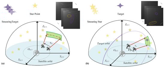
Figure 1.
Observation modes. (a) Star gazing mode: stars appear as points and RSOs as stripes. (b) Target gazing mode: the tracked RSO is a point and stars appear as stripes [8].
We focus on the star-gazing mode, illustrated in Figure 1a, where the observation platform maintains a fixed orientation relative to the celestial sphere. Due to their immense distance, stars exhibit negligible angular motion and thus appear as points. In contrast, RSOs orbiting the Earth have significant relative motion, causing their trajectories to be integrated over the exposure time and appear as distinct stripes [9]. The primary focus of this research is the detection of these stripe-like space resident targets under the star-gazing mode, a task we refer to as Stripe-like RSO Target Detection (SRTD).
The precise SRTD is critical for SSA and Space Traffic Management (STM) [10]. By interpreting a stripe’s geometric properties, such as length and orientation, one can extract kinematic data like velocity and motion vectors. This information is foundational for proactive STM tasks like collision warning and orbit prediction, elevating space surveillance from simple discovery to dynamic management. However, this detection task is complicated by two main challenges: environmental interference and the increasing number of RSOs.
1.1. Challenge 1: Complex Stray Light Interference
In the space environment, the detection of dim RSOs is severely hampered by complex stray light interference [4]. Long-exposure imaging, while necessary to capture dim targets, inevitably amplifies various types of environmental noise.
Specifically, intense background clutter arises from a diverse array of space stray lights and sensor disturbances, such as reflections from the Earth, Moon, and Sun, as well as dense star background interference shown in Figure 2. These interference sources manifest as non-uniform, high-intensity noise patterns that can overwhelm the faint signatures of RSOs [11]. Consequently, the targets are often submerged in the background with extremely weak contrast, making it difficult for standard detectors to distinguish valid stripe features from environmental disturbances.
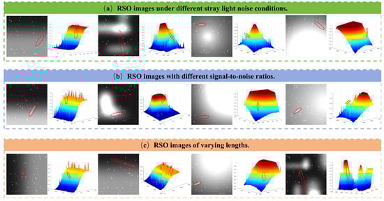
Figure 2.
Representative images of stripe-like targets (indicated by red dashed circles). (a) RSOs submerged in diverse complex stray light interferences. (b) RSOs under different stray light intensities. (c) RSOs with varying streak lengths.
1.2. Challenge 2: Dense and Overlapping Trajectories
The dramatic increase in the number of RSOs has led to the presence of many complex scenarios within the captured images [8]. In these scenarios, the trajectories of multiple RSOs overlap, making the precise detection of individual stripe-like targets difficult, as illustrated in Figure 3.
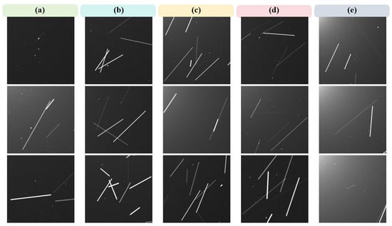
Figure 3.
Stripe-like targets in complex situations (a) Complex stellar and RSO combination patterns. (b) RSOs densely packed in the same direction. (c) RSOs with overlapping trajectories. (d) RSOs with strong signal strength contrast. (e) High noise background interference.
As can be seen in Figure 3, the dense accumulation of streaks, combined with their varying SNRs, makes it impossible to accurately identify each target. This constitutes another core challenge in the detection of stripe-like RSOs.
1.3. Limitations of Existing Methods
To address these challenges, existing research methods can be broadly categorized into three types [4,9,12]. However, traditional unsupervised methods [12,13] and semi-supervised learning strategies [14,15] often struggle in complex space environments. Relying on hand-crafted features or unstable pseudo-labels, these approaches lack the robustness to handle complex stray light interference and fail to adapt to variable target morphologies, resulting in limited generalization ability.
Consequently, deep networks based on fully supervised learning have become the mainstream approach due to their superior precision [16,17]. Nevertheless, current SOTA networks are predominantly optimized for generic or point-like infrared targets. They inherently lack the geometric modeling capabilities required to capture the dim features of stripe-like RSOs or to resolve the ambiguity of dense, overlapping trajectories. This fundamental mismatch between existing tools and the unique properties of RSOs highlights the urgent need for a specialized shape-aware architecture.
To effectively address the aforementioned challenges, we propose the Shape-Aware Attention Network (SAANet). The primary contributions are summarized as follows:
- We construct a specialized framework by integrating a streamlined Dense Nested Attention Network (DNANet) encoder with a Shape-Aware Feature Pyramid Network (SA-FPN). This design structurally embeds Two-way Orthogonal Attention (TTOA) to explicitly model linear topologies, efficiently preserving dim signals and overcoming complex interference bottlenecks.
- We propose an Adaptive Linear Oriented Bounding Box (AL-OBB) head. By formulating a joint geometric constraint mechanism via collinearity and aspect ratio, this strategy achieves precise target separation and localization, effectively resolving ambiguities in dense and intersecting scenarios.
- We perform extensive validation on the AstroStripeSet and StarTrails datasets. Results demonstrate that SAANet achieves SOTA performance, exhibiting superior accuracy and robustness compared to existing methods.
2. Materials and Methods
This section aims to review the related technologies, with a focus on discussing the traditional unsupervised learning paradigm, fully supervised learning strategies, and semi-supervised learning methods. By analyzing the limitations of these approaches in complex space environments, we identify the critical research gaps that motivate our proposed shape-aware framework.
2.1. Traditional Unsupervised Methods for SRTD
Traditional unsupervised methods for stripe-like target detection primarily solve the problem by designing specific features and filtering strategies. One such approach is the customized stripe pattern filtering method [18,19]. This method designs specific filter templates to match the expected stripe patterns in an image, thereby enabling the recognition and localization of stripe targets. It exhibits high efficiency and accuracy when dealing with specific targets that have a fixed morphology and well-defined features. However, due to the customized nature of the templates, this method struggles to adapt to the diversity of stripe targets. Its performance degrades sharply when the target’s shape or angle changes, and it is extremely sensitive to parameter settings.
Alternatively, methods based on morphological principles can be used [20]. For example, by applying morphological operations with a linear structuring element oriented parallel to the stripe’s direction, a stripe target can be enhanced while point-like stars and noise in the background are suppressed [21]. This approach demonstrates a certain degree of robustness when processing images with intense stray light interference. Nevertheless, its performance is heavily dependent on the design of the structuring element and it has difficulty adapting to the complex shapes and varying widths of stripe targets.
In summary, traditional unsupervised methods for SRTD are fundamentally limited by their reliance on rigid, hand-crafted geometric priors. This inflexibility prevents them from adapting to complex scenarios, as they struggle to disentangle overlapping targets and require separately designed filters for diverse backgrounds, ultimately leading to poor generalization and robustness.
2.2. Semi-Supervised Methods for Object Detection
In recent years, to address the challenge of large-scale data annotation, semi-supervised learning methods have been widely adopted in numerous fields, including object detection and image segmentation [1,2]. This paradigm significantly enhances a model’s generalization ability by combining a limited amount of labeled data with a large volume of unlabeled data.
Current mainstream semi-supervised learning approaches can be divided into two main categories: methods based on consistency regularization [22] and those based on pseudo-labeling [23,24]. Sajjadi et al. [22] first proposed the consistency regularization method, which compels the model to learn more robust feature representations by minimizing the prediction discrepancies between different perturbations of the same unlabeled data. The Mean Teacher framework is a classic example of this approach. However, such methods tend to be overconfident about low-quality or noisy labels, which affects the capture of the true structure of the data.
Lee et al. [23] first proposed the pseudo-labeling method, which utilizes a model trained on a small amount of labeled data to generate “pseudo-labels” for unlabeled data, subsequently incorporating this newly labeled data into the training process. The effectiveness of this approach is highly dependent on the quality of the pseudo-labels.
Early self-training methods were prone to errors due to incorrect pseudo-labels. To solve this problem, Liu et al. [25] and Xu et al. [26] introduced an end-to-end strategy based on the Mean Teacher (MT) framework [27], proposing the use of an Exponential Moving Average (EMA) mechanism to smooth the outputs of the teacher model. More recently, Zhu et al. introduced the MRSA-Net [28] and the CSDT semi-supervised framework to address SSTD under conditions of complex light pollution and data scarcity.
In summary, while semi-supervised learning reduces data annotation requirements, its performance is highly dependent on the quality of the unlabeled data. Since these methods rely on the model’s own predictions for self-supervision, they are prone to introducing and amplifying errors when data is noisy, leading to performance instability and limiting their reliability in complex SRTD scenarios.
2.3. Fully Supervised Methods for Object Detection
With the rise of Convolutional Neural Networks (CNNs), a number of deep learning-based methods for space object detection have been proposed. Unlike traditional methods that rely on hand-crafted filters, CNNs can automatically extract high-level abstract features from large-scale labeled data, allowing them to maintain excellent robustness when faced with diverse target morphologies and complex backgrounds.
Jia et al. [29] were the first to apply CNNs to space scenes, proposing a framework based on Faster R-CNN to classify point-like stars and stripe-like space objects. Wu et al. [30] proposed a simple yet effective “U-Net in U-Net” framework (UIU-Net), which embeds a smaller U-Net into a larger U-Net backbone. This design achieves multi-level [31], multi-scale representation learning for small infrared targets, addressing the issues of small target disappearance and limited feature differentiability in deep networks. To solve the problems of data scarcity and class imbalance in infrared small target detection, Sun et al. [32] constructed a large-scale dataset named IRDST and proposed a novel deep learning model called the Receptive Field and Direction-induced Attention Network (RDIAN). Li et al. [33] introduced a fully supervised method named the Dense Nested Attention Network (DNA) [33], which resolves the issue of small infrared target loss in deep networks by designing a Dense Nested Interactive Module (DNIM).
In essence, these fully supervised methods demonstrate the significant power of deep learning. By leveraging large-scale data, CNN-based approaches with innovative nested or attention-based architectures have proven highly effective for detecting small and dim targets. However, a critical review reveals that these state-of-the-art networks were predominantly designed for and evaluated on point-like small targets. Their architectural optimizations are therefore not tailored for targets with a distinct elongated morphology, such as the stripe-like RSOs central to the SRTD task. This fundamental mismatch between existing tools and the specific target shape constitutes a key research gap.
2.4. Summary of Related Works and Research Gap
In summary, existing methods for SRTD face significant limitations, revealing a clear research gap. Unsupervised methods lack robustness in complex backgrounds, while semi-supervised approaches are hampered by unreliable pseudo-labels. Even the most promising fully supervised methods are fundamentally mismatched for SRTD, as current architectures are designed for point-like targets and fail to address the unique elongated morphology and overlapping arrangements of RSOs. This highlights a critical need for a network architecture specifically tailored to the shape-aware detection of stripe-like targets.
Our research introduces and improves a network for infrared small target detection, directly addressing these methodological limitations and providing a more flexible, accurate, and computationally efficient approach for target detection. This allows for more precise detection of RSOs with a smaller number of parameters and floating-point operations.
3. Proposed Framework
To address the unique challenges of detecting stripe-like RSOs, we propose the SAANet. This architecture is established upon a unified Shape-Aware Paradigm, explicitly modeling the linear topology of targets. As illustrated in Figure 4, the framework comprises three theoretically aligned modules:
First, in the encoder stage, SAANet implements Streamlined Feature Maintenance to mitigate the loss of dim signals inherent in standard CNNs. By restructuring the DNANet encoder into a specialized feed-forward backbone without redundant upsampling, we ensure the high-fidelity preservation of faint features during the initial extraction phase.
Subsequently, in the decoder stage, to address the problem of traditional FPNs being shape-agnostic and diluting key morphological information, the multi-scale features are processed by our SA-FPN. Functioning as an Orthogonal Directional Modeler, this module structurally integrates TTOA to adaptively aggregate and enhance the target’s stripe-like morphology. This process transforms passive feature fusion into active topological refinement, offering a discriminative feature foundation for subsequent localization.
Finally, in the detection head stage, to resolve the inaccurate and unstable localization of elongated targets common with Horizontal Bounding Boxes (HBBs) [34] and standard Oriented Bounding Boxes (OBBs) [35], the feature pyramid is fed into the AL-OBB head. This module introduces a Joint Geometric Constraint Mechanism into the dynamic point set representation. By utilizing a linear-aware mechanism to impose strict collinearity and aspect ratio priors, it adaptively generates OBBs that are highly consistent with the physical morphology of RSOs, achieving precise separation and stable detection.

Figure 4.
SAANet Framework Diagram.
Figure 4.
SAANet Framework Diagram.

3.1. DNANet Encoder
Standard Convolutional Neural Networks (CNNs), such as ResNet, often cause the feature information of small, dim targets to be progressively lost in the deeper layers due to repeated pooling and strided convolutions. For stripe-like space objects that are only a few pixels wide, effectively preserving these dim signals is critically important. Therefore, we adopt the feature extraction philosophy of DNANet [31], which features a dense nested structure designed to prevent information loss. However, considering the specific characteristics of stripe-like targets and computational efficiency, we do not adopt the original architecture entirely. Instead, we introduce a streamlined version of the DNANet encoder, optimized to balance feature retention with inference speed.
3.1.1. Dense Nested Interactive Module
The Dense Nested Interactive Module (DNIM) is the core component of the encoder. Distinct from the original DNIM which employs tri-directional interactions (including bottom-up upsampling) between nodes, we implement a streamlined feed-forward structure, as illustrated in Figure 5. Specifically, we remove the computationally redundant upsampling pathways within the encoder to focus on pure feature extraction.
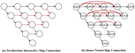
Figure 5.
U-shaped skip structure.
In our modified design, each node aggregates features mainly from shallower layers and the current layer. For the initial column (), the node receives features only from the previous layer via max-pooling:
where denotes a convolution operation, and denotes a max-pooling operation.
For nodes at deeper nested positions (), we simplified the interaction to receive inputs from only two directions: the same layer and the shallower layer. The computation is redefined as:
where denotes the concatenation operation. Note that the up-sampling term from the deeper layer present in the original DNANet is omitted here, and the input from the shallower layer is consistently processed via max-pooling to match the feature map resolution.
3.1.2. Cascaded Channel and Spatial Attention Module
To further enhance the representation of dim stripe-like targets, we integrate the Cascaded Channel and Spatial Attention Module (CSAM) into the convolutional blocks of our encoder. Based on the widely adopted Convolutional Block Attention Module (CBAM) design, this module sequentially infers attention maps along two separate dimensions: channel and spatial. By multiplying the input feature map with these attention maps, the network adaptively recalibrates features, emphasizing target-relevant information while suppressing background noise. This integration ensures that dim signals are amplified within the feature extraction stage, preventing them from being overwhelmed by background clutter.
3.2. Shape-Aware Feature Pyramid
Following the streamlined feature extraction, we propose the Shape-Aware Feature Pyramid Network (SA-FPN) to explicitly model the topological orientation of stripe-like targets. Standard Feature Pyramid Networks (FPN) rely on element-wise addition for feature fusion, which treats spatial information isotropically. However, this mechanism inherently dilutes the critical directional information required to distinguish stripe-like RSOs from noise. To overcome this theoretical limitation, we redesign the top-down pathway by constructing a shape-aware orthogonal fusion mechanism.
Instead of simple linear superposition, we structurally integrate the TTOA module [36] as the core fusion operator. Crucially, this integration establishes a global recursive directional refinement process. As illustrated in Figure 6, the SA-FPN accepts four hierarchical feature maps from the encoder as input. Through the top-down pathway, the high-level feature map is fused with the current stage features after upsampling to generate the pyramid levels . Additionally, to distinctively expand the receptive field for ultra-long trajectories, we generate a fifth level, , by applying max-pooling operation on . Consequently, the final output consists of five scale levels . This design ensures that the directional shape priors captured at coarser scales are explicitly propagated and preserved to guide the feature refinement at finer scales. By iteratively modeling row-wise and column-wise correlations across scales, SA-FPN transforms the fusion process from passive aggregation into active topological reconstruction.
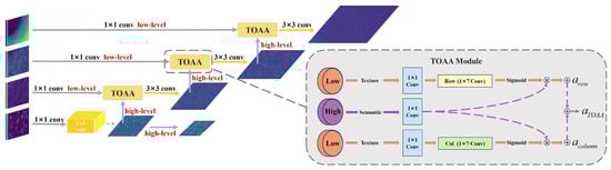
Figure 6.
Shape-Aware Feature Pyramid Network.
The detailed mechanism of the TTOA fusion unit is shown in Figure 6. It contains two parallel branches: one branch applies a deformable convolution to capture contextual information in the horizontal (row-wise) direction, while the other applies a deformable convolution to capture contextual information in the vertical (column-wise) direction. These attention maps then modulate the high-level features, effectively guiding the fusion process to focus on features consistent with the elongated structure of the target.
The output of the TTOA module, , is the sum of the outputs from the two attention branches: row and column:
The attention features for each direction are calculated as follows:
where is the Sigmoid function. is a bottleneck structure containing a convolution for noise and channel reduction. is a deformable convolution, is a deformable convolution, and ⊗ denotes element-wise multiplication. The kernel size k is a critical hyperparameter governing the receptive field of the TTOA module. A brief ablation study indicated that when , the receptive field fails to cover the full context of elongated stripe targets. Conversely, when , redundant background noise is introduced, interfering with feature aggregation. We found that setting effectively balances feature integrity and noise resistance, and thus adopted it as the default setting.
3.3. Adaptive Linear Oriented Bounding Box
While the dynamic point-set representation in DC-OBB offers flexibility for general object detection, it lacks specific geometric constraints for elongated objects, leading to unstable regression in dense RSO scenarios. To bridge this gap, we propose the AL-OBB detection head by incorporating a joint geometric constraint mechanism. This mechanism imposes a strong linear structure prior onto the adaptive point learning process. By forcing the representative points to align strictly with the target’s principal axis, our method resolves the ambiguity issues inherent in standard OBB approaches when dealing with high-aspect-ratio and overlapping trajectories.
The workflow of the AL-OBB detection head is divided into two closely coupled stages. The first is the generation and conversion of an adaptive point set, where a representative point set learned by the network is transformed into an OBB that precisely encloses the target. The second stage is a quality assessment and selection process based on enhanced linear awareness, which further ensures that the selected bounding box accurately reflects the elongated and directional characteristics of the stripe-like target. A detailed flowchart of this process is shown in Figure 7.
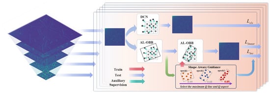
Figure 7.
Overall configuration of AL-OBB.
Through this approach, the AL-OBB detection head provides more accurate and stable detection results for elongated targets, making it particularly suitable for application scenarios where traditional HBB and OBB methods perform poorly.
3.3.1. Adaptive Point Learning
First, for each potential target in the image, a set of representative points is generated that can flexibly describe its morphology. Specifically, the detection head employs a Dynamic [26] Convolutional Network (DCN) to learn a position-dependent offset for each location on the feature map. At each location, we predefine an initial regular grid of N = 9 points as
where represents the 2D coordinates of the k-th initial point for the i-th potential target.
Simultaneously, the network learns a set of offsets, , which are applied to this initial grid to adjust it, resulting in the final adaptive representative point set, . This process can be expressed by the following formula:
This adaptive approach allows the point set to distribute itself freely according to the target’s actual shape and orientation, greatly enhancing the fitting capability for stripe-like targets with variable morphologies. After obtaining the adaptive point set , which accurately outlines the target’s contour, we convert it into a final OBB using standard computational geometry algorithms.
First, the minimum convex hull of the point set is constructed using an algorithm such as the Jarvis March, ensuring that all representative points are contained within it. Subsequently, the Rotating Calipers algorithm is applied to the convex hull to efficiently find the enclosing rectangle with the minimum area that envelops the hull. This minimum-area enclosing rectangle is the desired OBB, denoted as .
3.3.2. Joint Geometric Constraint Mechanism
The Joint Geometric Constraint Mechanism is the theoretical core of the AL-OBB head, distinguishing it from general-purpose object detectors. We posit that for a point set to accurately represent a stripe-like RSO, merely satisfying collinearity is insufficient, as it fails to distinguish between a compact noise cluster and an elongated streak. Therefore, we formulate a novel joint quality metric, , which integrates two orthogonal geometric dimensions: collinearity and aspect ratio. This metric functions as a shape-aware regularizer during the learning process, comprehensively evaluating the topological consistency of the predicted point set.
The first step is to quantify how closely the spatial distribution of approximates a straight line, evaluating the collinearity of the point set as the basis for an initial metric. First, the centroid of the point set is calculated, and all points are centralized to obtain , as computed by the following formulas:
where .
Subsequently, we calculate the second-order moments of the centralized point set, , , , and construct the covariance matrix C of the point set:
These values are then used to construct an initial metric, , which is highly sensitive to collinearity. Its calculation formula is as follows:
where [35] represents an initial, unnormalized collinearity score whose value increases sharply as the point set approaches collinearity, since its denominator is related to the determinant of the covariance matrix which approaches zero. The terms are the second-order central moments of the centralized point set, respectively, used to describe its degree of dispersion. Finally, (epsilon) is a very small positive number (e.g., ) used to prevent division by zero and ensure the numerical stability of the computation.
To facilitate network optimization, we use an exponential function to smoothly map the initial score into the interval , yielding the final collinearity quality metric, :
where is a tunable positive hyperparameter that controls the steepness of the normalization function.
However, collinearity alone is insufficient to describe a stripe. A point-like noise artifact or a compact cluster of points could also achieve a high collinearity score. Therefore, in the second step of this mechanism, we introduce an aspect ratio metric to explicitly encourage elongated morphologies. This metric is inspired by the core idea of Principal Component Analysis (PCA).
We construct the covariance matrix from the centralized point set and solve for its two eigenvalues, and (ensuring that ). Based on these, we define the aspect ratio quality metric, :
where and are the largest and smallest eigenvalues of the covariance matrix, respectively. precisely reflects the variance or degree of spread of the point set along its principal axis (i.e., the direction of the stripe’s length), while reflects the variance along the minor axis (i.e., the direction of the stripe’s width). For an ideal stripe, is significantly larger than . The term (epsilon) is, likewise, a very small positive number included to ensure numerical stability.
Finally, we multiply the collinearity metric and the aspect ratio metric to fuse them into a more robust, comprehensive, and accurate joint quality metric, :
The enhanced metric, , provides a highly precise geometric prior for the network’s learning process. During training, only those point sets that are both highly collinear and have an elongated morphology can achieve a final high score approaching 1, thereby occupying a dominant role in the loss function calculation. This mechanism effectively compels the model to generate representative points that precisely delineate the complete morphology of RSOs, laying a solid theoretical foundation for achieving superior localization and regression precision in complex space environments.
3.4. Loss Function
The training process of SAANet is guided by a joint loss function, , which is designed to simultaneously optimize target classification, localization, and the spatial distribution of the representative point set. The total loss function is composed of a weighted sum of three components: the classification loss, [37]; the localization loss, [38]; and the spatial constraint loss, [35]:
The weighting hyperparameters , and were determined through an empirical grid search on the validation set to balance the gradient magnitudes of different loss terms. Based on the experimental results, we set to ensure stable model convergence.
3.4.1. Classification Loss
The classification loss term is used to distinguish between targets (stripes) and the background. Due to the severe class imbalance problem, where background pixels far outnumber target pixels in the images, we adopt the Focal Loss. The Focal Loss reduces the weight of well-classified, easy samples, forcing the model to focus more on learning hard-to-distinguish samples during training.
where represents the total number of points in a batch, and is the model’s predicted probability for the ground-truth class. The parameter is a balancing factor used to adjust the contribution weight of positive versus negative samples. The parameter is a modulating factor; when , it reduces the contribution of well-classified samples with high prediction probabilities () to the total loss.
3.4.2. Localization Loss
The localization loss term measures the geometric discrepancy between the predicted bounding box, which is converted from the representative point set, and the ground-truth OBB. We employ a loss function based on the Generalized Intersection over Union (GIOU) because it not only considers the overlapping area but also accounts for the non-overlapping regions, making it more effective at handling cases where the boxes do not overlap.
The calculation of GIOU relies on the standard Intersection over Union (IoU), which is defined as follows:
where A and B represent the predicted bounding box and the ground-truth bounding box, respectively, and C is the smallest convex set that encloses both A and B.
The localization loss, , is thus given by:
where represents the number of point sets in a batch that are assigned as positive samples.
3.4.3. Spatial Constraint Loss
The spatial constraint loss term is a key regularization term that ensures the adaptively learned representative points fall within the target region instead of being scattered outside of it. It enforces this constraint by penalizing any representative points that lie outside the ground-truth bounding box. The penalty function, , is defined as follows:
where represents the distance between the representative point and the geometric center of the ground-truth bounding box, .
With the penalty function defined, we can now formulate the full spatial constraint loss, :
where represents the total number of positive samples in a batch.
4. Experiment
This chapter aims to comprehensively evaluate the performance of our proposed SAANet on the task of detecting stripe-like RSOs. We begin by detailing the experimental setup, including the datasets, evaluation metrics, and implementation details. Subsequently, we demonstrate the superiority of SAANet through quantitative and qualitative comparisons with several state-of-the-art infrared target detection models and the traditional ResNet50. Finally, we conduct a series of thorough ablation studies to validate the effectiveness of each innovative component within our model.
4.1. Experimental Setup
4.1.1. Dataset
To address the challenges posed by the complex spatial situations involving stripe-like RSOs, we conducted extensive experiments on two datasets, each presenting distinct characteristics and challenges.
AstroStripeSet [28]: This dataset was specifically constructed for the task of stripe-like space object detection. It comprises images affected by four typical types of space stray light: Earthlight, Sunlight, Moonlight, and mixed light. The complete dataset contains 1500 images of size 256 × 256, divided into a fixed set of 1000 training images, 100 validation images, and 400 test images. The dataset simulates varying exposure durations through different streak lengths. This variation in signal intensity, combined with complex stray light backgrounds, allows for a comprehensive verification of the model’s robustness under diverse exposure and noise interference conditions.
StarTrails Dataset [8]: This dataset was built for space object detection in a scanning imaging mode, generated by simulating the motion and imaging processes of stars and space objects combined with time delay integration technology. The entire dataset consists of 2000 images of size 1024 × 1024, containing over 70,000 valid RSO annotations. To simulate specific exposure levels, the dataset is explicitly parameterized with 32, 64, 96, and 128 integration stages [8], resulting in targets with inconsistent signal intensities and streak lengths. This configuration, combined with a high density of overlapping and intersecting trajectories, serves as a rigorous benchmark for assessing a detection model’s ability to precisely discriminate and localize dense, arbitrarily oriented targets in complex environments.
The AstroStripeSet and StarTrails Dataset are derived from benchmarks established in [8,28]. We strictly adhered to their original data partitioning and annotation protocols for fair comparison. The datasets are available at https://github.com/Lyy-7/SAANet (accessed on 5 January 2026).
4.1.2. Evaluation Metrics
To quantitatively evaluate the model’s performance, we adopted widely recognized evaluation metrics from the field of object detection, including Recall and Average Precision (AP).
First, we introduce Recall, which is a metric that measures the model’s ability to find all existing targets. It is defined as the ratio of the number of correctly detected positive samples to the total number of actual positive samples:
where TP is the number of correctly detected targets, and FN is the number of actual targets that the model failed to detect.
Additionally, we introduce the AP metric to provide a comprehensive evaluation of the model’s Precision and Recall for a single class. It measures the model’s overall performance by calculating the weighted average of precision at various recall levels.
4.1.3. Implementation Details
Our proposed SAANet model and all comparative experiments were implemented based on the MMRotate open-source toolbox and the PyTorch (version 1.11.0) deep learning framework. To ensure a consistent experimental environment, all models were trained and tested on a single server equipped with an NVIDIA RTX 4090 GPU.
We employed the Stochastic Gradient Descent (SGD) optimizer with an initial learning rate set to 0.008. To accommodate the characteristics of the different datasets, input images were uniformly resized to a fixed dimension. For the AstroStripeSet, the input size was pixels with a batch size of 16. For the StarTrails dataset, owing to its higher original resolution and sparser targets, the input size was set to pixels with a batch size of 2. Furthermore, to enhance the model’s generalization ability, we applied data augmentation techniques during the training phase, primarily consisting of random horizontal, vertical, and diagonal flips. We intentionally excluded geometric rotations to prevent interpolation artifacts from degrading the structural integrity of faint, pixel-level stripe targets. Furthermore, since the datasets already contain complex, real-world stray light interference, we avoided adding synthetic noise to preserve the realistic noise distribution characteristics. All models were trained for 100 epochs.
4.2. Comparative Experiments
To comprehensively evaluate the performance of SAANet, we conducted extensive comparative experiments against a diverse set of baselines. In the category of traditional methods, we selected representative algorithms including TopHat [39], MaxMedian [40], LCM [41], the Frangi Filter [42], and the recent tensor-based DDCF [43]. For deep learning comparisons, we employed the classic ResNet50 [44] as a baseline, alongside several state-of-the-art networks optimized for dim object detection, such as ISNet [36], MSHNet [45], ISTDUNet [46], LW-IRSTNet [47], and SARATRNet [48]. This evaluation encompasses quantitative, qualitative, and ablation analyses on both the AstroStripeSet and StarTrails datasets to verify the effectiveness and robustness of the proposed framework.
4.2.1. Analysis on AstroStripeSet
As presented in Table 1, SAANet achieves optimal performance across most evaluation metrics. The quantitative results clearly demonstrate the limitations of traditional approaches for this task. Relying on hand-crafted features, these methods struggle in complex stray light environments. As shown in the table, methods like LCM and Frangi yield limited performance. Even the latest tensor-based method DDCF, while outperforming classical filters, only attains a Recall of 0.613 and an AP of 0.478. In contrast, SAANet achieves a Recall of 0.930 and an AP of 0.864, representing a substantial performance leap over traditional baselines. This validates that data-driven deep networks are essential for distinguishing dim targets from complex backgrounds.

Table 1.
Performance comparison on the AstroStripeSet. The notation “Red” indicates the best performance in each category (closest to Gts for Dets).
Among deep learning approaches, SAANet consistently outperforms both the classic ResNet50 baseline and representative SOTA networks. While ResNet50 and ISTDUNet show competitive performance with Recalls of 0.877 and 0.897, they lack specific mechanisms for orientation regression, limiting their AP to around 0.77. Notably, compared to SOTA networks like MSHNet and SARATRNet which are optimized for infrared small targets, SAANet achieves a significant lead of 7.6% and 17.9% in AP respectively. This superiority stems from the Shape-Aware Paradigm which explicitly models the linear topology that generic small target detectors fail to capture.
Regarding detection quantity, SAANet generates 406 detection boxes, a figure remarkably close to the ground truth count of 400. This high level of consistency demonstrates the exceptional precision of the model and its capability to effectively suppress false alarms. In comparison, networks such as SARATRNet and ISTDUNet generate 502 and 470 candidates respectively, indicating a higher incidence of false positives in noisy backgrounds. Under detailed illumination conditions, SAANet exhibits exceptional robustness. It achieves the highest performance in Moon Light and Earth Light scenarios with Recalls of 0.960 and 0.920 respectively, and maintains the top AP of 0.856 even under intense Sun Light interference.
Figure 8 presents a qualitative comparison of the proposed SAANet against several competing networks. The visual results demonstrate the superior detection capability and robustness of our method.
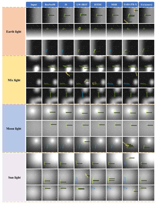
Figure 8.
Comparison of Detection Results for Stripe-like RSOs in AstroStripeSet. Green boxes indicate successful detections. Blue boxes highlight missed targets, whereas yellow boxes denote false alarms.
The performance gap is most evident under complex scenarios such as cluttered Mix Light and low-illumination Moon Light. When strong interfering light causes a sharp increase in background interference, networks like MSHNet and LW-IRSTNet exhibit significant missed detections. Although ISNet and ISTDUNet show relatively high precision, they generate incomplete bounding boxes, failing to effectively preserve target integrity. In stark contrast, SAANet demonstrates exceptional robustness, precisely detecting dim targets missed by other methods while maintaining their structural continuity.
Even under relatively clearer conditions like Earth Light and Sun Light, competing networks still exhibit limitations. Specifically, in scenarios dominated by intense Sun Light, the strong background radiance creates severe interference. Comparative methods, such as MSHNet and SARATRNet, struggle to distinguish between this high-intensity stray light noise and valid targets, resulting in noticeable false alarms. While SAANet maintains robustness, the misclassification by other models highlights the severity of strong stray light influence in these environments. Meanwhile, ResNet50 and ISNet suffer from missed detections due to weak feature extraction. Furthermore, even when competing networks successfully detect targets, their detection precision is inferior to that of SAANet.
Collectively, the visual results across all conditions validate the advanced capabilities of the Shape-Aware Paradigm in handling dim and obscured targets and confirm its strong generalization performance in diverse space imaging environments.
4.2.2. Analysis on StarTrails Dataset
As detailed in Table 2, SAANet demonstrates outstanding performance on the StarTrails dataset. Traditional methods struggle severely in this scenario characterized by dense and overlapping trajectories. Methods like LCM and Max-Median achieve an Average Precision of less than 0.26. Even the latest method DDCF [43] and the tubular-specific Frangi Filter fail to yield satisfactory results, achieving APs of only 0.332 and 0.391, respectively. This highlights the inability of hand-crafted features to disentangle complex geometric intersections in high-density environments.
Table 2.
Performance comparison on the StarTrails dataset. The notation “Red” indicates the best performance in each category.
In the deep learning category, SAANet leads all competing networks with a Recall of 0.850 and an AP of 0.815. It is worth noting that while recent SOTA networks like MSHNet and SARATRNet perform well on small targets, they show limited effectiveness on this dataset with APs of 0.739 and 0.730 respectively. This suggests that architectures optimized for point-like targets may fail to capture the orientation features required for dense stripes. SAANet surpasses the runner-up ISTDUNet by 1.2% in AP, validating the effectiveness of the proposed joint geometric constraint mechanism in resolving overlapping ambiguities.
An analysis of detection counts further underscores the superior quality of candidates generated by SAANet. As detailed in the table, SAANet yields 7965 detections, a figure that most closely aligns with the ground truth count. In contrast, LW-IRSTNet and SARATRNet produce notably fewer detections, specifically 6956 and 7084. These reduced counts correlate directly with their lower recall rates, indicating that these models fail to detect a significant portion of valid targets. Conversely, ISTDUNet generates an excessive 9150 candidates, which implies a propensity for false alarms within cluttered regions. By maintaining a detection count that is highly consistent with the ground truth, SAANet achieves an optimal trade-off between precision and recall, demonstrating its robustness in accurately localizing valid targets while effectively suppressing background noise in dense environments.
The macroscopic qualitative results in Figure 9 corroborate the quantitative findings. Distinct from the multi-color error analysis in Figure 8, we adopt a prediction-only protocol for the StarTrails dataset to directly assess regression consistency. The visualizations reveal that classic networks like ResNet50 and ISNet, along with recent methods such as MSHNet and SARATRNet, struggle with the dataset’s complexity, yielding numerous missed detections and false alarms. Although ISTDUNet achieves a relatively high recall rate, its performance is compromised by a large number of cluttered and fragmented detection boxes. In contrast, SAANet demonstrates a clear advantage, striking an optimal balance between a high detection rate and clean, precise results. It is important to note that due to the extremely high target density in this dataset, explicitly marking all detection errors in the global view would result in severe visual occlusion. Therefore, we focus on the macroscopic distribution here. While SAANet exhibits superior global coverage, it still encounters challenges in regions with explosive trajectory density, where signal saturation can lead to occasional missed detections.
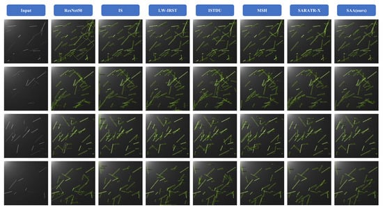
Figure 9.
Detection Visualization for Stripe-like RSOs on the StarTrails Dataset. Green boxes represent the network’s prediction outputs.
To provide a more in-depth analysis, Figure 10 presents a magnified view of several typical challenging scenarios. In the case of overlapping trajectories (a), competing networks often produce fragmented detections or fail to disentangle the intersection. SAANet, however, maintains the structural integrity of each target. Similarly, for densely packed RSOs (b), other models exhibit low precision or incorrectly merge adjacent targets, while SAANet accurately separates each object, demonstrating a superior understanding of spatial relationships. However, a specific limitation persists in these ultra-dense intersections. When multiple trajectories intersect at narrow angles, the significant spatial overlap may trigger the Non-Maximum Suppression mechanism to incorrectly suppress valid adjacent bounding boxes, resulting in minor discontinuities.
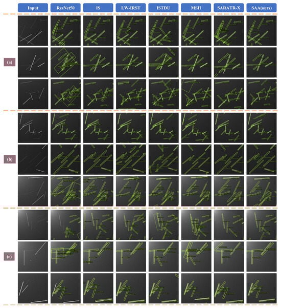
Figure 10.
Magnified Comparison of Stripe-like RSO Detection Results on the StarTrails Dataset. Green boxes represent the network’s prediction outputs. (a) RSOs with overlapping trajectories. (b) RSOs densely packed in the same direction. (c) RSOs with strong signal strength contrast against high noise background interference.
Finally, in the high-noise environment (c), while networks like SARATRNet generate false alarms and ResNet50 misses dim targets, our model achieves an optimal balance, detecting both strong and weak-signal targets while effectively suppressing noise. Collectively, these extensive qualitative comparisons validate the exceptional performance and robustness of the SAANet when handling dense, overlapping, and interference targets.
4.2.3. Ablation Study
In this section, we conduct a series of comprehensive ablation studies to systematically evaluate the effectiveness of the core modules within our proposed framework. To quantify the contribution of each component to the final performance, we trained different model configurations on the AstroStripeSet and StarTrails datasets. The detailed experimental results are summarized in Table 3.
Table 3.
Comprehensive ablation study of each component in SAANet.
Our analysis begins with the baseline model. Equipping the baseline model with the SA-FPN and CSAM modules significantly enhances performance. On the AstroStripeSet, it achieves substantial gains of 11.5% in Recall and 13.1% in AP, while on the StarTrails dataset, the AP is also boosted by approximately 9.5%. This series of improvements fully validates the designated role of SA-FPN as a powerful decoder and CSAM as a feature enhancer, proving their exceptional effectiveness in capturing the dim image features of stripe-like RSOs.
Furthermore, to verify the effectiveness of the proposed joint geometric constraints, we analyze the internal mechanisms of the AL-OBB head. Here, and denote the collinearity and aspect ratio constraints in the AL-OBB head, respectively. As shown in Table 3, applying either or individually yields performance improvements compared to the configuration without geometric constraints. However, the consistent and significant gains are maximized when both constraints are applied jointly. This highlights the core value of the AL-OBB module: it successfully imposes effective constraints on the linear features of the targets, thereby generating more precise detection boxes that are better suited to the unique geometry of stripe-like objects.
Finally, when all modules including SA-FPN, CSAM, and the complete AL-OBB are integrated simultaneously, our complete model achieves optimal performance across all metrics on both datasets. On AstroStripeSet, it reaches a Recall of 0.930 and an AP of 0.864, while on StarTrails, it achieves a Recall of 0.850 and an AP of 0.815. This result profoundly validates the effectiveness of our proposed Unified Shape-Aware Paradigm: the explicit modeling of linear topologies by SA-FPN and the joint geometric constraint mechanism of AL-OBB are tightly coupled to successfully resolve the core challenges of complex stray light interference and dense overlapping trajectories, thereby establishing the SOTA performance of SAANet in space stripe-like object detection tasks.
4.2.4. Model Efficiency Analysis
In practical space-based applications, the computational resources and storage capacity of satellite platforms are extremely limited. Therefore, in addition to detection precision, we evaluated the model’s parameters (Params), floating-point operations (FLOPs), and inference speed (FPS). The experiments were conducted on an NVIDIA RTX 4090 GPU with a unified input size of .
The quantitative results in Table 4 highlight the significant advantages of SAANet in terms of model lightweighting. Its parameter count is only 11.22 M, which is approximately one-third of the standard ResNet50. More critically, compared to the Transformer-based SARATRNet, SAANet’s parameter count is only about 15% of the former, drastically reducing the demand for on-orbit storage space. Regarding computational complexity, although SAANet introduces attention mechanisms to effectively capture faint stripe features, resulting in a higher computational load than some other SOTA networks, its 105.92 G FLOPs remains far below the computationally intensive ISTDUNet and is on par with MSHNet and LW-IRSTNet.
Table 4.
Comparison of model complexity and inference speed. The arrows ↓ and ↑ indicate that lower and higher values are better, respectively.
Considering the precision performance in Table 1 and Table 2, SAANet achieves optimal detection performance with a lower storage cost and reasonable computational cost. This balance between precision and efficiency makes it a highly competitive solution for space situational awareness tasks.
A comprehensive analysis synthesizing the efficiency metrics in Table 4 with the detection precision in Table 1 and Table 2 reveals that SAANet achieves the highest Average Precision of 0.864 on the AstroStripeSet and 0.815 on the StarTrails dataset, while maintaining a moderate footprint of 11.22 M parameters and 105.92 G FLOPs. In contrast, although SARATRNet exhibits a higher inference speed, its extensive parameter count of 75.06 M yields substantially lower accuracies of 0.681 and 0.730. Similarly, LW-IRSTNet, despite having the smallest parameter size, attains APs of only 0.566 and 0.773, indicating limited generalization capability. This comparison demonstrates that SAANet utilizes parameters more efficiently to capture stripe-like features. Consequently, the optimal balance between precision and efficiency positions SAANet as a highly competitive solution for space situational awareness tasks.
5. Conclusions
In this work, we propose the Shape-Aware Attention Network (SAANet) to address the challenges of detecting stripe-like Resident Space Objects (RSOs). To tackle the limitations of standard detectors in complex stray light and dense environments, we establish a unified shape-aware paradigm with three core contributions. First, we implement streamlined feature maintenance by restructuring the encoder into a specialized feed-forward backbone, ensuring the preservation of dim signals. Second, we construct a shape-aware orthogonal fusion mechanism within the Shape-Aware Feature Pyramid Network (SA-FPN), explicitly modeling linear topologies to enhance feature discriminability. Third, we propose a joint geometric constraint mechanism in the Adaptive Linear Oriented Bounding Box (AL-OBB) head. By enforcing strict collinearity and aspect ratio alignment, this strategy theoretically resolves regression ambiguities in overlapping scenarios.
Extensive experiments on the AstroStripeSet and StarTrails datasets demonstrate that SAANet achieves state-of-the-art performance. Specifically, on the AstroStripeSet, it achieves a Recall of 0.930 and an Average Precision (AP) of 0.864, while on the StarTrails dataset, it attains a Recall of 0.850 and an AP of 0.815. Qualitative analysis further confirms its robustness in maintaining target integrity and suppressing noise. This work provides an effective theoretical and practical solution for Space Situational Awareness (SSA), offering new avenues for the detection of morphologically specific targets.
Although the datasets used in this study rigorously simulate space environments, we acknowledge the necessity of validation on real-world observational imagery. Due to the extreme scarcity of public, accurately annotated real-world datasets for stripe-like RSOs, we will dedicate future work to acquiring such data to further verify the generalization capability of the proposed model.
Author Contributions
Conceptualization, Y.L. and H.L.; methodology, Y.L.; software, Y.L. and X.S.; validation, Y.M.; investigation, Y.Z.; data curation, Z.C.; writing—original draft preparation, X.S.; writing—review and editing, H.L.; visualization, Y.L.; supervision, R.Z.; funding acquisition, R.Z. All authors have read and agreed to the published version of the manuscript.
Funding
This work was supported by the Sichuan Science and Technology Program under Grant No. 2025ZNSFSC1504.
Data Availability Statement
The data presented in this paper will be released soon.
Acknowledgments
Thanks to the accompaniers working with us in department of the Institute of Optics and Electronics, Chinese Academy of Sciences.
Conflicts of Interest
The authors declare no conflicts of interest.
References
- Guo, X.; Chen, T.; Liu, J.; Liu, Y.; An, Q. Dim Space Target Detection via Convolutional Neural Network in Single Optical Image. IEEE Access 2022, 10, 52306–52318. [Google Scholar] [CrossRef]
- Li, M.D.; Xiao, S.P.; Chen, S.W. Polarimetric ISAR Space Target Structure Recognition Based on Embedded Scattering Mechanism and Semi-Supervised Representation Learning. IEEE Trans. Geosci. Remote Sens. 2025, 63, 5102019. [Google Scholar] [CrossRef]
- Chen, Y.; Tang, Q.y.; He, Q.g.; Chen, L.t.; Chen, X.w. Review on Hypervelocity Impact of Advanced Space Debris Protection Shields. Thin-Walled Struct. 2024, 200, 111874. [Google Scholar] [CrossRef]
- Liu, D.; Wang, X.; Xu, Z.; Li, Y.; Liu, W. Space Target Extraction and Detection for Wide-Field Surveillance. Astron. Comput. 2020, 32, 100408. [Google Scholar] [CrossRef]
- Sun, B.; Zhang, Y.; Zhou, Q.; Zhang, X. Effectiveness of Semi-Supervised Learning and Multi-Source Data in Detailed Urban Landuse Mapping with a Few Labeled Samples. Remote Sens. 2022, 14, 648. [Google Scholar] [CrossRef]
- Wu, D.; Dell’Elce, L.; Rosengren, A.J. RSO Proper Elements: Concept, Methods, and Application to Maneuver Detection. Adv. Space Res. 2024, 73, 64–84. [Google Scholar] [CrossRef]
- Felt, V.; Fletcher, J. Seeing Stars: Learned Star Localization for Narrow-Field Astrometry. In Proceedings of the 2024 IEEE/CVF Winter Conference on Applications of Computer Vision (WACV), Waikoloa, HI, USA, 3–8 January 2024; pp. 8282–8290. [Google Scholar] [CrossRef]
- Fu, Z.; Lei, Y.; Tang, X.; Xu, T.; Tian, G.; Gao, S.; Du, J.; Yang, X. Oriented Clustering Reppoints for Resident Space Objects Detection in Time Delay Integration Images. IEEE Trans. Geosci. Remote Sens. 2024, 62, 5650715. [Google Scholar] [CrossRef]
- Lévesque, M.P. Automatic Reacquisition of Satellite Positions by Detecting Their Expected Streaks in Astronomical Images. In Proceedings of the Advanced Maui Optical and Space Surveillance Technologies Conference, Maui, HI, USA, 1–4 September 2009. [Google Scholar]
- Hilton, S.; Sabatini, R.; Gardi, A.; Ogawa, H.; Teofilatto, P. Space traffic management: Towards safe and unsegregated space transport operations. Prog. Aerosp. Sci. 2019, 105, 98–125. [Google Scholar] [CrossRef]
- Lu, K.; Li, H.; Lin, L.; Zhao, R.; Liu, E.; Zhao, R. A Fast Star-Detection Algorithm under Stray-Light Interference. Photonics 2023, 10, 889. [Google Scholar] [CrossRef]
- Jiang, P.; Liu, C.; Yang, W.; Kang, Z.; Li, Z. Automatic Space Debris Extraction Channel Based on Large Field of View Photoelectric Detection System. Publ. Astron. Soc. Pac. 2022, 134, 024503. [Google Scholar] [CrossRef]
- Levesque, M.P.; Buteau, S. Image Processing Technique for Automatic Detection of Satellite Streaks; Defense Technical Information Center: Fort Belvoir, VA, USA, 2007. [Google Scholar]
- Chen, Z.; Wang, R.; Xu, Y. Semi-Supervised Remote Sensing Building Change Detection with Joint Perturbation and Feature Complementation. Remote Sens. 2024, 16, 3424. [Google Scholar] [CrossRef]
- Guan, D.; Xing, Y.; Huang, J.; Xiao, A.; El Saddik, A.; Lu, S. S2Match: Self-paced Sampling for Data-Limited Semi-Supervised Learning. Pattern Recognit. 2025, 159, 111121. [Google Scholar] [CrossRef]
- Liu, L.; Niu, Z.; Li, Y.; Sun, Q. Multi-Level Convolutional Network for Ground-Based Star Image Enhancement. Remote Sens. 2023, 15, 3292. [Google Scholar] [CrossRef]
- Zhang, T.; Cao, S.; Pu, T.; Peng, Z. AGPCNet: Attention-Guided Pyramid Context Networks for Infrared Small Target Detection. arXiv 2021, arXiv:2111.03580. [Google Scholar] [CrossRef]
- Jiang, P.; Liu, C.; Yang, W.; Kang, Z.; Fan, C.; Li, Z. Space Debris Automation Detection and Extraction Based on a Wide-field Surveillance System. Astrophys. J. Suppl. Ser. 2022, 259, 4. [Google Scholar] [CrossRef]
- Cegarra Polo, M.; Yanagisawa, T.; Kurosaki, H. Real-Time Processing Pipeline for Automatic Streak Detection in Astronomical Images Implemented in a Multi-GPU System. Publ. Astron. Soc. Jpn. 2022, 74, 777–790. [Google Scholar] [CrossRef]
- Xi, J.; Wen, D.; Ersoy, O.K.; Yi, H.; Yao, D.; Song, Z.; Xi, S. Space Debris Detection in Optical Image Sequences. Appl. Opt. 2016, 55, 7929–7940. [Google Scholar] [CrossRef]
- Filho, J.; Duarte, P.; Gordo, P.; Peixinho, N.; Melicio, R.; Valério, D.; Gafeira, R. Space Surveillance Payload Camera Breadboard: Star Tracking and Debris Detection Algorithms. Adv. Space Res. 2023, 72, 4215–4228. [Google Scholar] [CrossRef]
- Sajjadi, M.; Javanmardi, M.; Tasdizen, T. Regularization With Stochastic Transformations and Perturbations for Deep Semi-Supervised Learning. In Proceedings of the Advances in Neural Information Processing Systems, Barcelona, Spain, 5–10 December 2016; Curran Associates, Inc.: New York, NY, USA, 2016; Volume 29. [Google Scholar]
- Lee, D.H. Pseudo-Label: The Simple and Efficient Semi-Supervised Learning Method for Deep Neural Networks. In Proceedings of the ICML 2013 Workshop: Challenges in Representation Learning (WREPL), Atlanta, GA, USA, 16–21 June 2013. [Google Scholar]
- Sohn, K.; Zhang, Z.; Li, C.L.; Zhang, H.; Lee, C.Y.; Pfister, T. A Simple Semi-Supervised Learning Framework for Object Detection. arXiv 2020, arXiv:2005.04757. [Google Scholar] [CrossRef]
- Liu, Y.C.; Ma, C.Y.; He, Z.; Kuo, C.W.; Chen, K.; Zhang, P.; Wu, B.; Kira, Z.; Vajda, P. Unbiased Teacher for Semi-Supervised Object Detection. arXiv 2021, arXiv:2102.09480. [Google Scholar] [CrossRef]
- Xu, M.; Zhang, Z.; Hu, H.; Wang, J.; Wang, L.; Wei, F.; Bai, X.; Liu, Z. End-to-End Semi-Supervised Object Detection with Soft Teacher. In Proceedings of the IEEE/CVF International Conference on Computer Vision, Montreal, BC, Canada, 11–17 October 2021; pp. 3060–3069. [Google Scholar]
- Tarvainen, A.; Valpola, H. Mean Teachers Are Better Role Models: Weight-averaged Consistency Targets Improve Semi-Supervised Deep Learning Results. In Proceedings of the Advances in Neural Information Processing Systems, Long Beach, CA, USA, 4–9 December 2017; Curran Associates, Inc.: New York, NY, USA, 2017; Volume 30. [Google Scholar]
- Zhu, Z.; Zia, A.; Li, X.; Dan, B.; Ma, Y.; Long, H.; Lu, K.; Liu, E.; Zhao, R. Collaborative Static-Dynamic Teaching: A Semi-Supervised Framework for Stripe-like Space Target Detection. Remote Sens. 2025, 17, 1341. [Google Scholar] [CrossRef]
- Jia, P.; Liu, Q.; Sun, Y. Detection and Classification of Astronomical Targets with Deep Neural Networks in Wide-field Small Aperture Telescopes. Astron. J. 2020, 159, 212. [Google Scholar] [CrossRef]
- Wu, X.; Hong, D.; Chanussot, J. UIU-Net: U-Net in U-Net for Infrared Small Object Detection. IEEE Trans. Image Process. 2023, 32, 364–376. [Google Scholar] [CrossRef] [PubMed]
- Ronneberger, O.; Fischer, P.; Brox, T. U-Net: Convolutional Networks for Biomedical Image Segmentation. In Proceedings of the Medical Image Computing and Computer-Assisted Intervention—MICCAI 2015, Munich, Germany, 5–9 October 2015; Navab, N., Hornegger, J., Wells, W.M., Frangi, A.F., Eds.; Springer: Cham, Switzerland, 2015; pp. 234–241. [Google Scholar] [CrossRef]
- Sun, H.; Bai, J.; Yang, F.; Bai, X. Receptive-Field and Direction Induced Attention Network for Infrared Dim Small Target Detection with a Large-Scale Dataset IRDST. IEEE Trans. Geosci. Remote Sens. 2023, 61, 5000513. [Google Scholar] [CrossRef]
- Li, B.; Xiao, C.; Wang, L.; Wang, Y.; Lin, Z.; Li, M.; An, W.; Guo, Y. Dense Nested Attention Network for Infrared Small Target Detection. arXiv 2022, arXiv:2106.00487. [Google Scholar] [CrossRef]
- Chen, S.; Wang, H.; Shen, Z.; Wang, K.; Zhang, X. Convolutional Long-Short Term Memory Network for Space Debris Detection and Tracking. Knowl.-Based Syst. 2024, 304, 112535. [Google Scholar] [CrossRef]
- Li, W.; Chen, Y.; Hu, K.; Zhu, J. Oriented RepPoints for Aerial Object Detection. In Proceedings of the 2022 IEEE/CVF Conference on Computer Vision and Pattern Recognition (CVPR), New Orleans, LA, USA, 18–24 June 2022; pp. 1819–1828. [Google Scholar] [CrossRef]
- Zhang, M.; Zhang, R.; Yang, Y.; Bai, H.; Zhang, J.; Guo, J. ISNet: Shape Matters for Infrared Small Target Detection. In Proceedings of the 2022 IEEE/CVF Conference on Computer Vision and Pattern Recognition (CVPR), New Orleans, LA, USA, 18–24 June 2022; pp. 867–876. [Google Scholar] [CrossRef]
- Lin, T.Y.; Goyal, P.; Girshick, R.; He, K.; Dollar, P. Focal Loss for Dense Object Detection. In Proceedings of the IEEE International Conference on Computer Vision, Venice, Italy, 22–29 October 2017; pp. 2980–2988. [Google Scholar]
- Rezatofighi, H.; Tsoi, N.; Gwak, J.; Sadeghian, A.; Reid, I.; Savarese, S. Generalized Intersection Over Union: A Metric and a Loss for Bounding Box Regression. In Proceedings of the IEEE/CVF Conference on Computer Vision and Pattern Recognition, Long Beach, CA, USA, 15–20 June 2019; pp. 658–666. [Google Scholar]
- Rivest, J.F.; Fortin, R.A. Detection of dim targets in digital infrared imagery by morphological image processing. Opt. Eng. 1996, 35, 1886–1893. [Google Scholar] [CrossRef]
- Deshpande, S.D.; Er, M.H.; Venkateswarlu, R.; Chan, P. Max-mean and max-median filters for detection of small targets. In Proceedings of the SPIE’s International Symposium on Optical Science, Engineering, and Instrumentation, Denver, CO, USA, 18–23 July 1999. [Google Scholar]
- Chen, C.L.P.; Li, H.; Wei, Y.; Xia, T.; Tang, Y.Y. A Local Contrast Method for Small Infrared Target Detection. IEEE Trans. Geosci. Remote Sens. 2014, 52, 574–581. [Google Scholar] [CrossRef]
- Frangi, A.F.; Niessen, W.J.; Vincken, K.L.; Viergever, M.A. Multiscale Vessel Enhancement Filtering. In Proceedings of the Medical Image Computing and Computer-Assisted Intervention—MICCAI’98, Cambridge, MA, USA, 11–13 October 1998; Wells, W.M., Colchester, A., Delp, S., Eds.; Springer: Berlin/Heidelberg, Germany, 1998; pp. 130–137. [Google Scholar]
- Xie, F.; Yang, D.; Yang, Y.; Wang, T.; Zhang, K. Infrared Small Target Detection Using Directional Derivative Correlation Filtering and a Relative Intensity Contrast Measure. Remote Sens. 2025, 17, 1921. [Google Scholar] [CrossRef]
- Zhang, D.; Zhang, X.; Yin, Z.; Xie, Y.; Wei, H.; Chang, Z.; Li, W.; Zhang, D. mmRotation: Unlocking Versatility of a Single mmWave Radar via Azimuth Panning and Elevation Tilting. IEEE Trans. Mob. Comput. 2025, 24, 6045–6061. [Google Scholar] [CrossRef]
- Liu, Q.; Liu, R.; Zheng, B.; Wang, H.; FU, Y. Infrared Small Target Detection with Scale and Location Sensitivity. In Proceedings of the 2024 IEEE/CVF Conference on Computer Vision and Pattern Recognition (CVPR), Seattle, WA, USA, 16–22 June 2024; pp. 17490–17499. [Google Scholar] [CrossRef]
- Hou, Q.; Zhang, L.; Tan, F.; Xi, Y.; Zheng, H.; Li, N. ISTDU-Net: Infrared Small-Target Detection U-Net. IEEE Geosci. Remote Sens. Lett. 2022, 19, 7506205. [Google Scholar] [CrossRef]
- Kou, R.; Wang, C.; Yu, Y.; Peng, Z.; Yang, M.; Huang, F.; Fu, Q. LW-IRSTNet: Lightweight Infrared Small Target Segmentation Network and Application Deployment. IEEE Trans. Geosci. Remote Sens. 2023, 61, 5621313. [Google Scholar] [CrossRef]
- Li, W.; Yang, W.; Hou, Y.; Liu, L.; Liu, Y.; Li, X. SARATR-X: Toward Building a Foundation Model for SAR Target Recognition. IEEE Trans. Image Process. 2025, 34, 869–884. [Google Scholar] [CrossRef]


Disclaimer/Publisher’s Note: The statements, opinions and data contained in all publications are solely those of the individual author(s) and contributor(s) and not of MDPI and/or the editor(s). MDPI and/or the editor(s) disclaim responsibility for any injury to people or property resulting from any ideas, methods, instructions or products referred to in the content. |
© 2026 by the authors. Licensee MDPI, Basel, Switzerland. This article is an open access article distributed under the terms and conditions of the Creative Commons Attribution (CC BY) license.