Highlights
What are the main findings?
- ZELIG and SRT can be feasibly coupled for efficiently simulations of forest logging dynamics.
- ZELIG-SRT coupled model provides a physical-based approach for post-logging biomass change estimation from annual satellite imagery.
What are the implications of the main findings?
- The ZELIG-SRT model provides a framework for quantitative simulation of biomass changes and corresponding canopy spectral changes before and after forest logging, which can be used for analyzing the spectral response mechanism of forest logging.
- The post-logging biomass change can be estimated from annual optical satellite imagery by an efficient physical-based model, which is more interpretable than empirical methods and gives no need for complex scenario simulations.
Abstract
The abundant satellite data have enabled the study of the dynamics of forest logging and its corresponding carbon balance with remote sensing. Change detection techniques with moderate-resolution imagery have been widely developed. Yet the signal processing or machine learning methods are sample-dependent, lacking an understanding of spectral signals of forest growth and logging cycles, which is necessary to distinguish logging from other types of disturbance, and mechanism models addressing post-logging tree changes are too complex for parameter inversion. We therefore proposed an efficient physical-based model for spectral simulation of annual forest logging by coupling forest dynamic model ZELIG and the stochastic radiative transfer (SRT) model. The forest logging simulation was conducted and validated by Abies forest field data before and after logging in Wangqing County, Northeastern China (R2 = 0.85, RMSE = 10.82 t/ha). The spectral changes in Abies forest stands with annual growth and varying logging intensities were simulated by the novel model. The annual Landsat-8 and Gaofen-1 fusion multispectral imagery of the study area from 2013 to 2016 was furtherly used to extract annual sequence spectral data of 350 forest plots and perform inversion of the annual difference in above-ground biomass (dAGB). With the inversion method combining the look-up table of the ZELIG-SRT model and the random forest regression, the retrieved dAGB of the 350 plots indicated consistency with the measured data on the whole (R2 = 0.71, RMSE = 13.32 t/ha). The novel physical-based approach for AGB monitoring is more efficient than previous 3D computer models and less dependent on field samples than data-driven models. This study provides a theoretical basis for understanding the remote sensing response mechanism of forest logging and a methodological basis for improving forest logging monitoring algorithms.
1. Introduction
Moderate logging is an essential measure of forest management, while excessive deforestation is a common disturbance that damages the forest ecosystem. The annual changes in forest above-ground biomass (AGB) caused by logging can reflect the evolution of forest ecosystems and the dynamics of forest carbon balance. Timely acquisition of spatiotemporal distribution information on the occurrence and intensity of post-logging AGB changes is an important prerequisite for forest management and forest ecosystem protection. The techniques for automatic monitoring of forest disturbance using moderate-resolution imagery have been widely studied based on the development of change detection algorithms from time-series imagery, such as LandTrendR [1], TimeSync [2], the Vegetation Change Tracker [3], the Continuous Change Detection and Classification (CCDC) [4], and Breaks for Additive Season and Trend (BFAST) [5]. Change detection algorithms have been applied in multiple forest logging areas, achieving good monitoring results [6,7,8,9,10,11,12]. However, the extraction of forest disturbance information in temporal spectra has been mostly based on signal processing or machine learning methods, which have a strong dependence on spectral normalization, time-series fitting algorithms, and parameter selection, lacking an understanding of spectral signals of forest growth and logging cycles. As a result, it is still a challenge to distinguish logging from other types of disturbance and to propose an efficient model for different forest types. Therefore, clarifying the mechanism of remote sensing signal changes before and after logging is the basis for accurately interpreting forest logging information in remote sensing images. It is necessary to utilize mechanism models to accurately simulate the temporal remote sensing signals of forest logging cycles.
The forest dynamic model simulates the changes in tree species composition and major tree parameters (such as biomass, productivity, volume, age, tree height, diameter) during the growth, management, and succession processes of forest stands based on forest physiology and ecological processes. The radiative transfer model explains the transmission process of radiation through surface features in a physical way, which is an important foundation for understanding the relations between remote sensing signals and various forest parameters. With the changes in logging scenarios simulated by the forest dynamic model and the changes in remote sensing signals simulated by the radiative transfer model, the coupled model can provide a large number of time-series remote sensing dynamic simulations of forest scenarios. Currently, it has been used for single-phase forest parameter inversion [13,14,15,16], but has not been applied in forest logging monitoring. One of the important issues is that time-series signal simulation needs to consider the changes in different spatiotemporal dimensions, which requires both the matching degree between forest dynamic models and radiative transfer models, as well as high computational efficiency for both. At present, classic analytical models (e.g., PROSAIL) and 3D computer simulation models (e.g., DART) both reveal certain problems in dynamic model coupling [17,18]. The turbid medium assumption of the classic analytical models struggles to match the post-logging tree changes output by the forest dynamic model. Although 3D computer models show high accuracy, the precision of scene characterization needs to be achieved at the cost of the running speed, which restricts large-scale and long-term applications.
To overcome the limits in simulation efficiency of previous 3D computer models, this study provides a novel efficient approach for model coupling, using a 3D analytical model instead of a computer simulation model. The stochastic radiative transfer (SRT) model, rooted in the 3D radiative transfer equation, introduces stochastic probability parameters to parameterize the 3D scene structure [19]. The averaging procedure of 3D scenarios results in the parameterization of the equation in terms of two stochastic moments of a vegetation structure. The first stochastic moment is the probability of finding leaf elements at a specific canopy depth; the second moment is the pair correlation function, the joint probability of finding leaf elements at two specific canopy depths along the defined direction. In this approach, SRT achieves a balance between the concise 1D form and the accurate 3D simulation [20]. SRT has been applied in the production of MODIS LAI (Leaf Area Index), FPAR (Fracture of Photosynthetically Active Radiation) products, and Gaofen-1 LAI products [21,22]. The initial version of SRT was aimed at single-species forests and had the ability to simulate the radiative transfer of discontinuous forest canopies composed of discrete tree crowns [19]. After the proposal of SRT theory, it has undergone a series of developments, including the parameterization of the three-dimensional structure of forest stands with various crown shapes through the improvement of stochastic geometry theory [23], the integration of the gap ratio and leaf area index into the model by coupling the Beer Lambert law [24], the correction of specular reflection and hotspot effects [25,26], and the addition of solar-induced chlorophyll fluorescence radiative transfer [27]. In terms of expanding the heterogeneous forest canopy structure, the SRT model has been extended to include the Stochastic Mixture Radiative Transfer (SMRT) model for multi-species mixed forests [28] and the Stochastic Radiative Transfer model for forests with a heterogeneous canopy structure (ESRT) [20], which can be used for forests with different complex structures. In previous comparative studies on the simulations of SRT and 3D computer models, the computational efficiency of SRT was approximately 4 to 10 times that of computer models (varies with scene size), and there was no need to generate a 3D forest scene before computation [19,20,27]. The dimensionality reduction of model parameters greatly improves operational efficiency, and at the same time, its input parameters that express the scene highly match the output scene of the forest dynamic model, thus having great potential in time-series simulation.
Therefore, we coupled the forest dynamic model ZELIG [29] and the SRT model in this study to simulate forest logging and validated the model based on forest field survey data and satellite images from two phases before and after logging in Wangqing County, Northeastern China in 2015. And based on the proposed model, the spectral changes during the forest harvesting cycle were simulated and analyzed. With the novel coupled model, a model-based monitoring method of forest logging was proposed by combining the look-up table and random forest regression, which was based on the time-series simulation of remote sensing signals for a large number of forest logging scenarios. The annual difference in above-ground biomass (dAGB) in the study area was estimated using multi-temporal fusion imagery of Landsat-8 and Gaofen-1. The accuracy of dAGB estimation was verified by two-phase field survey data of Abies forest sample plots. This study aims to provide a theoretical basis for understanding the remote sensing response mechanism of forest logging, as well as improving physical-based forest logging monitoring algorithms, so they are both efficient and less dependent on field samples.
2. Materials and Methods
2.1. Study Area and Data Acquisition
The study area is located in Jingouling Forest Farm of Wangqing Forestry Bureau, Jilin Province, China (130°05′~130°20′E, 43°17′~43°25′N), with an altitude of about 762 m. As in the northern temperate monsoon zone, the annual average temperature is about 3.9 °C, the annual precipitation is 600–700 mm, and the plant growth period is about 120 days. The soil type is mainly dark brown soil. The main coniferous tree species in the study area include Abies nephrolepis (Trautv.) Maxim., Picea jezoensis var. microsperma (Lindl.) Cheng et L.K. Fu, Pinus koraiensis Sieb. et Zucc., and Larix olgensis Henry. The main broad-leaved tree species include Betula platyphylla Suk., Tilia amurensis Rupr., Betula costata Trautv., Fraxinus mandshurica Rupr., Populus ussuriensis Kom., and Acer mono Maxim.
The study area is a typical region of Northeast China for forest logging and management. Twelve permanent plots of 100 m × 100 m were set in the study area in August 2013. In January 2015, tree logging operations were carried out in nine of the plots, while the other three control plots were not operated. The logging mode was guided by crop tree management. In such mode, 100~150 uniformly distributed crop trees were selected in each 100 m × 100 m plot, and the logged trees were selected around the crop trees, which may disturb their growth. Each plot was divided into 100 small sample plots of 10 m × 10 m. The sample plots were surveyed twice, in August 2013 and August 2016, to obtain measured data before and after logging. Each time, trees with a diameter at breast height of 1 cm or more in the sample plots were measured, and information such as the tree number, relative spatial coordinates, tree species, diameter at breast height (D), tree height (H), branch height, crown width, etc., were recorded. The above-ground biomass (AGB) of each tree was calculated by D and H according to the published Chinese standard of tree biomass models. The boundary of the sample plots and the locations of all the individual trees were recorded by a real-time kinematic (RTK) positioning system, of which the positioning accuracy was 5 cm.
Among 1200 sample plots of 10 m × 10 m, a total of 350 sample plots with the main tree species of Abies nephrolepis (plant ratio > 65%) were selected as the study object of this article (Figure 1). The modeling of complex mixed forests was not the focus in this study. Due to the fact that leaf spectra change with the growth status of trees, it is not possible to obtain real-time in situ leaf spectral data during the logging year. In order to enhance the universality and repeatability of this study, we obtained a total of 200 reflectance and transmittance data of Abies foliage from the EcoSIS public dataset [30,31,32], and we took the average value as the Abies foliage spectral data (Figure 2). We downloaded the 30 m resolution multispectral remote sensing images of Landsat-8 and the 2 m resolution panchromatic images of Gaofen-1 during the cloud-free growing season from 2013 to 2025 in the study area. The Landsat-8 bands used in this study included six bands: Blue (450–515 nm), Green (525–600 nm), Red (630–680 nm), Near-Infrared (845–885 nm), Shortwave Infrared 1 (1560–1660 nm), and Shortwave Infrared 2 (2100–2300 nm). We used the Gram Schmidt Pan Sharpening tool of ENVI software (Environment for Visualizing Images, Version 5.6, developed by Exelis Visual Information Solutions) for image fusion to obtain the annual 2 m resolution multispectral fusion images. Note that the imagery from 2013 to 2025 provided validation of ZELIG-SRT for dynamic spectral simulations, and only the imagery from 2013 to 2016 were used for dAGB inversion.
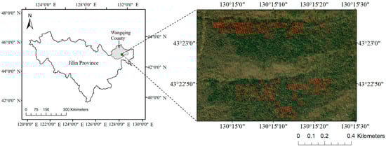
Figure 1.
The study area and sample plots of Abies forests (red squares).
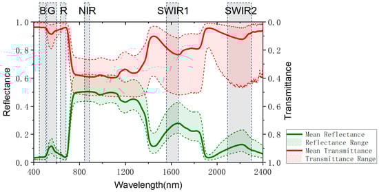
Figure 2.
The reflectance/transmittance of Abies foliage for the six bands corresponding to Landsat-8.
2.2. Coupling of ZELIG and SRT
2.2.1. Model Description of ZELIG and SRT
The ZELIG model mainly consists of two parts: the module of tree physiological factors and the module of environmental factors limiting tree growth. Among them, the tree physiological factor module includes a single-tree growth model, single-tree death model, and single-tree renewal model. The module on limiting tree growth by environmental factors includes the light factor limiting equation, soil moisture limiting equation, soil fertility limiting equation, and temperature limiting equation. When simulating forest succession using the ZELIG model, the input parameters are divided into two parts: the biophysical parameters of the simulated target tree species and the environmental constraints of the simulated succession process. Specifically, the biophysical parameters of the simulated target tree species include the maximum growth age (Amax), maximum growth diameter at breast height (Dmax), maximum growth tree height (Hmax), growth rate (G), minimum and maximum effective accumulated temperature (DDmin, DDmax), shade tolerance level (Light), drought tolerance level (Drt), and fertility tolerance level (Nutri). In terms of environmental constraints, the monthly average temperature and monthly cumulative precipitation are the main inputs of the ZELIG model. After simulation, the ZELIG model outputs the annual growth parameters of all individual trees in the sample plot, including tree species, diameter at breast height, tree height, crown length, leaf area, etc.
The SRT model utilizes the statistical technique to average the 3D radiative regime of forests into a 1D form, providing the equation directly for the mean radiation field [19]. The averaging procedure results in the parameterization of the equation in terms of two stochastic moments of the vegetation structure. The first stochastic moment is the probability, p(z), of finding leaf elements at canopy depth z; the second moment is the pair-correlation function, q(z,z′,Ω), the joint probability of finding leaf elements at depth z and z′ along the direction Ω. In this study, the 3D stochastic canopy structure was based on the following assumptions: (1) crowns are modeled as identical cylinders; and (2) all the crown centers are generated following a stationary Poisson point process [33]. The major input variables of the SRT model are (1) solar illumination variables—solar zenith angle and the ratio of direct-to-total incident flux; (2) canopy geometry, including height and horizontal dimensions of cylindrical crowns; (3) statistical moments of canopy structure, namely, p and q; (4) foliage properties—leaf area volume density, leaf normal orientation distribution, foliage reflectance, and transmittance spectra; (5) soil reflectance spectra. The output of SRT is the canopy reflectance, which corresponds to the surface reflectance pixels of moderate-resolution satellite imagery.
For ZELIG, both pure forests and mixed forests can be addressed for growth simulation. However, the ecological effects of mixed tree species will increase the difficulty of model calibration. For SRT, the model assumption is set for pure forests. The extension version of SMRT/ESRT has been proposed for mixed forests at the cost of more computing time. To propose and test an efficient framework for model coupling, we focused on relatively pure forests and considered only the main species of the sample plots in this study.
2.2.2. Method of Model Coupling
Theoretically, with the annual forest structure parameters output by ZELIG, the annual canopy reflectance can be simulated by SRT. However, in order to conduct the simulations of annual canopy reflectance during the forest logging cycle, two technical issues need to be addressed for model coupling. On the one hand, forest logging, as well as forest growth, should be realized in the ZELIG model; on the other hand, the outputs of ZELIG and the inputs of SRT should be matched one by one.
We simulated forest logging by modifying the single-tree mortality model. In the logging mode of crop tree management, the crop trees generally followed a uniform distribution. We assumed that the logged trees around the crop trees were also uniformly distributed. The specific method is to add an additional random term when simulating whether each tree dies in each simulated year. The logging year is selected based on the rotation period. The probability of the random term is determined by the logging intensity, which indicates the ratio of the number of logged trees to the total number of trees. For example, if 20% of the logging is carried out every 10 years, a random number between 0 and 1 is generated for each tree in the 10n year. If it is less than 0.2, it is considered that the single tree has been logged.
We derived the functions of SRT inputs according to the connotation and empirical relationship in forestry. The complete set of plot parameters output by the ZELIG model can provide input parameters for the SRT model. The conversion relationship between output and input parameters is listed in Table 1. The canopy coverage is a function of the density and radius of tree crowns in the case of Poisson germ-grain models [23]. The optical crown height varies with the ground cover of LAI, which means that for a specific stand LAI, an increase in canopy coverage is accompanied by a decrease in the within-crown foliage density [34]. The pair correlation function indicates the probability of photons colliding with crowns simultaneously at different layers in a specific direction, which is determined by the coverage (p) and spatial distribution (AR) of vegetation elements. The detailed derivation of the functions can be checked in [19,20].

Table 1.
The conversion relationship between ZELIG outputs and SRT inputs.
2.3. Model Evaluation
Simulating the dynamic changes in forest growth and logging processes that are close to reality is the key to the accuracy of the ZELIG and SRT coupled model. In order to evaluate the performance of the coupled model, the sample plot measured data of Abies forests were utilized to calibrate and validate the forest dynamic, and the spectral signals for the forest harvesting cycle were simulated for sensitivity analysis.
2.3.1. Model Calibration and Validation
The application of the ZELIG model requires calibration of the physiological and ecological input parameters of the forest stand to keep consistent with the actual situation of the forest stand in the study area. To adjust the tree species parameters of the ZELIG model using the measured data of Abies trees, the specific steps are as follows: (1) The initial situation of the sample plot was input based on the measured data of the sample plot in 2013. The logging situation of various plots was input according to the logging data of 2016 plots (Figure 3). The temperature and precipitation input parameters were obtained from the local meteorological data website (Table 2). (2) As some physiological parameters are calculated through a series of complex dynamic equations and are difficult to directly measure, this study mainly referred to the physiological parameter settings of similar tree species in the relevant Chinese literature. (3) The method for correcting uncertain parameters in the model involved repeatedly adjusting the sensitive parameters within an appropriately continuous range to ensure a good correlation between the estimated values of the model and the observed values of the sample plot. The specific parameter settings are shown in Table 3. ZELIG simulation was conducted to estimate forest stand parameters three years later, and the R2 and RMSE were used for verification of the accuracy between the estimated AGB and the measured AGB of the 2016 plots.
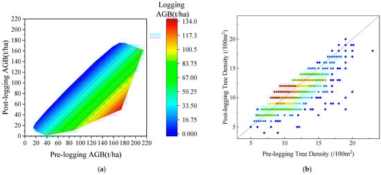
Figure 3.
The distribution of pre- and post-logging AGB (a) and tree density (b) of the sample plots.
Table 2.
The meteorological data of Wangqing county.
Table 3.
The specific biophysical parameters of Abies.
After calibration of ZELIG parameters, we randomly chose a total of 10 sample plots with different levels of logging intensity to simulate the annual canopy reflectance from 2013 to 2025. The reference annual canopy reflectance of the 10 sample plots was extracted from the multispectral fusion images of Landsat-8 and Gaofen-1, so as to validate the spectral simulations of ZELI-SRT.
2.3.2. Simulation of Spectral Signals for Forest Harvesting Cycle
In order to provide a baseline analysis for applications of logging monitoring, we implemented the analysis on the sensitivity of optical signals in response to the logging intensity during the forest management cycle. In forest management, the logging intensity is determined comprehensively by the management purpose, stand characteristics, site conditions, and economic factors. In order to cover different forest management and disturbance patterns, we generated 11 groups of Abies forests for the simulation of growth and logging dynamics. The simulation of each group suggests a forest management period of 150 years, with a selective cutting cycle every 10 years. For the 11 forest groups, the intensity of selective cutting ranging from 0% to 100%, respectively. The annual changes in forest AGB, the corresponding canopy reflectance in six bands of Landsat-8, and seven canopy spectral indices (Table 4) were simulated. The computation time was recorded to evaluate the model efficiency with a processing platform of Intel Core i7–7700 HQ, 4 cores, and 8 GB memory.
Table 4.
The equations of the spectral indices.
2.4. Quantitative Estimation of Post-Logging dAGB
To further explore the potential application of the proposed model in quantitative parameter inversion before and after forest logging, we used satellite multispectral imagery of the study area from 2013 to 2016 to extract annual canopy spectral data of the Abies sample plots and perform annual AGB inversion. The inversion method was based on the ZELIG-SRT model simulations combined with random forest (RF) regression.
(1) Look-up table (LUT) construction. Based on the ZELIG-SRT model, we simulated the annual sequence dataset. The reflectance and transmission spectra of Abies leaves were set as five gradients based on 200 measured spectra in the dataset, namely the mean, maximum, minimum, and two quartiles, which were resampled according to the spectral response function of Landsat-8 into six spectral bands. We selected three regions from the image that are close to bare ground and extracted their pixel reflectance as three types of soil reflectance. The annual forest logging intensity was set according to the method in Section 2.3.2, and other stand parameters were set according to the study area parameters in Section 2.3.1, with the sun and view direction being the same as the corresponding remote sensing image. A total of 24,750 samples were generated in the LUT (Table 5). The output canopy reflectance bands were consistent with the spectral bands of Landsat-8, and thus the annual AGB and the corresponding canopy reflectance were simulated for each scene.
Table 5.
The parameter settings of the LUT inputs.
(2) Feature variable selection. The canopy reflectance of 6 bands and 7 spectral indices (Table 4) was used as feature variables. We used the Boruta function package in R software to perform nonlinear selection of feature variables, with the annual differences in reflectance of 6 bands and 7 spectral indices in the look-up table as explanatory variables and the annual difference in AGB (dAGB) as the dependent variable. The number of decision trees ntree in the Boruta model was set as 150 for the stability of the model, while other parameters remained default. The features of relatively higher importance were selected for inversion.
(3) Inversion of dAGB. Based on the look-up table simulation and the feature selection, an RF regression model was built using the simulated dAGB and the selected spectral features of the 4-year change sequence data. The RF model can rank the explanatory variables based on their ability to predict the target variable [42], and a 5-fold cross-validation method was used to verify the robustness of the model trained on the dataset. The annual variation in the selected spectral features of the sampled remote sensing images was input into the random forest model. The dAGB in each sample site was retrieved. The observed dAGB in the field survey sample sites was used as the true value to verify the accuracy of the inversion model. The modeling and retrieving process was carried out using the MATLAB (v2022a) toolbox “Random Forest”. The retrieving accuracy was evaluated using R2 and RMSE.
In order to further evaluate the performance of the inversion approach, a comparative experiment was conducted. We constructed a similar RF model but directly using the spectral features of the 4-year imagery instead of the LUT, and we tested the ability to invert dAGB by the 5-fold cross-validation method.
3. Results
3.1. Simulation Accuracy of Forest Logging Dynamic
Based on the 350 forest plots and logging data from 2013, the forest AGB in 2016 was simulated (Figure 4). The simulation results of dAGB are highly consistent with the measured dAGB for two phases. Overall, there is some underestimation of simulated values, especially when the forest logging intensity is higher. This may be explained by the fact that the simulated forest stands were only with the consideration of the main tree species, Abies, and other broad-leaved companion tree species may result in higher-than-simulated biomass growth in the forest stands. The annual canopy NDVI of the selected 10 sample plots was simulated from 2013 to 2025 (Figure 5). The overall trend of the simulated annual NDVI is consistent with the imagery, especially around the logging year of 2015. The post-logging changes in NDVI (2015–2025) can reveal the process of vegetation restoration. The forests may suffer other sources of disturbances in the restoration process, which can explain the higher simulated NDVI than that extracted in certain years.
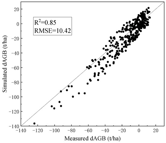
Figure 4.
The results of dAGB simulation by ZELIG with the calibration of sample plot parameters.
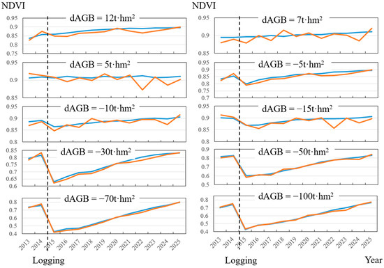
Figure 5.
The annual canopy NDVI from 2013 to 2025 of 10 sample plots with different logging intensities in 2015. dAGB indicates the difference between the biomass in 2016 and 2013. The blue line represents simulated NDVI of ZELIG-SRT, and the orange line denotes the extracted NDVI from imagery.
3.2. Spectral Changes in Canopy During Forest Harvesting Cycle
According to the forest harvesting cycle set in this study (Figure 6), the variation curves of reflectance in the six bands (Figure 7) and the seven spectral indices (Figure 8) of the forest canopy were simulated during the 11 groups of a 150-year forest management cycle. Forest growth and logging have opposing effects on canopy spectra, and the changes in spectral indices become more severe with an increasing logging intensity. The reflectance of the NIR band increases with forest growth and decreases with logging, while the reflectance trends of other bands are the opposite; such a phenomenon can be explained by Figure 2. In the NIR band, vegetation exhibits strong reflection and transmission, and there are weak absorption characteristics, resulting in an increase in canopy reflectance with the increase in vegetation; in other bands, vegetation has a strong ability to absorb light, resulting in a decrease in canopy reflectance with the increase in vegetation. The spectral changes before and after logging provide knowledge for interpreting temporal optical images of forest stands in logging regions, and they can provide a modeling basis for further exploration of remote sensing monitoring technology for forest logging.
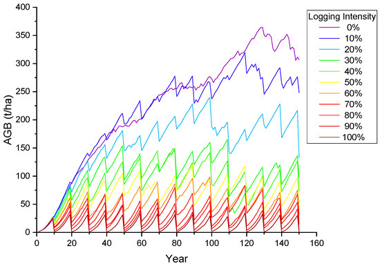
Figure 6.
The annual change in the forest AGB during the simulated forest harvesting cycle.
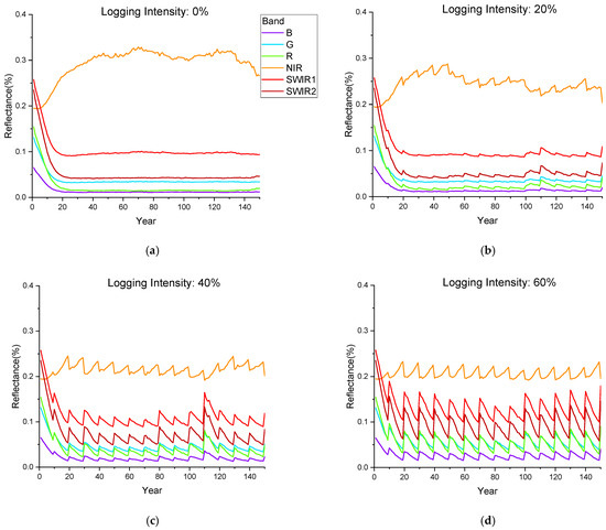
Figure 7.
The annual change in canopy reflectance during the simulated forest harvesting cycle for the six bands corresponding to Landsat-8. (a–d) represent the stands with logging intensities of 0%, 20%, 40% and 60%, respectively.
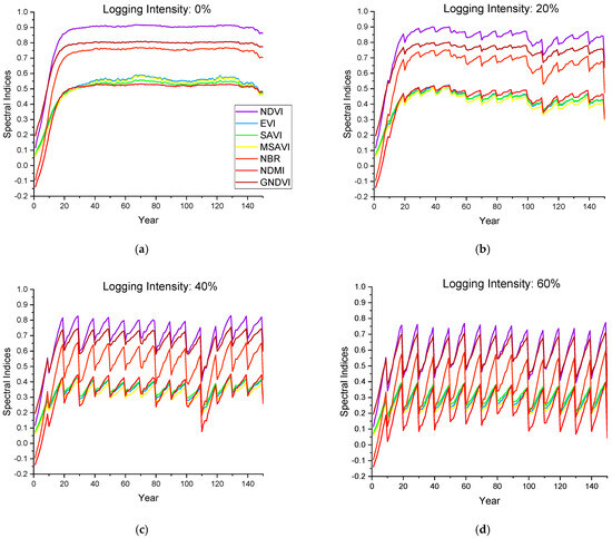
Figure 8.
The annual change in the canopy spectral indices during the simulated forest harvesting cycle. (a–d) represent the stands with logging intensities of 0%, 20%, 40% and 60%, respectively.
For each 150-year simulation of ZELIG-SRT, the total computation time is approximately 148 s (about 1 s for ZELIG and 147 s for SRT). The computation time of SRT for one scenario is about 0.98 s.
3.3. Importance Rank of Spectral Features
Relative importance can evaluate the contribution of feature variables to the model, providing a reference for nonlinear selection of remote sensing variables. Figure 9 shows the rank of remote sensing variables extracted from this study. The top-ranked remote sensing variables mainly include NIR, EVI, MSAVI, and SAVI, which are mainly composed of near-infrared band reflectance and the soil-adjusted vegetation indices, indicating that the NIR band information and the background-weakened indices have better sensitivity to forest dAGB.
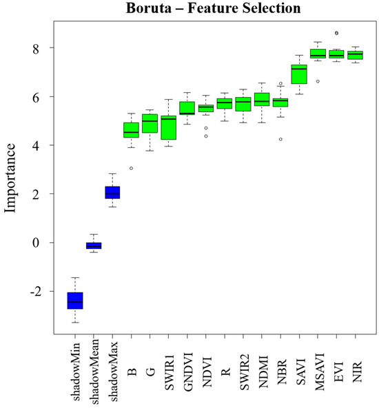
Figure 9.
The importance rank of the selected features based on Boruta.
3.4. Inversion of dAGB from the Infusion Images
For the ZELIG-SRT approach, the inversion results of the dAGB of the 350 plots indicated consistency with the measured data on the whole (Figure 10a). The R2 between the retrieved values and the measured values is 0.71. The AGB reductions are underestimated when the logging intensity is high. This may be due to the fact that the resilience of real forests after logging is stronger than the assumption of pure forests. The sample plots are not 100% pure forests, as the mixed structure formed by associated tree species increases the restoration ability of the forest stand. The spectral changes caused by logging have been weakened by forest restoration.
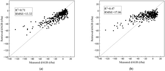
Figure 10.
The results of dAGB retrieval for the 350 sample plots of Abies forests: (a) the ZELIG-SRT approach; (b) the comparative RF approach.
For the comparative RF approach, the inversion bias of the dAGB was higher than the ZELIG-SRT approach (Figure 10b). The spectral changes may be affected by multiple factors, such as initial forest conditions and soil background, other than the dAGB. Compared with the complex LUTs that consider physical mechanisms, it is difficult to reveal the spectral response of biomass changes using simple machine learning models.
4. Discussion
The ZELIG-SRT coupled model provides an efficient physical-based approach for post-logging biomass change estimation from annual satellite imagery. The advantages of this study lie in the following: (1) A coupling framework between the three-dimensional analytical model SRT and the forest dynamic model is proposed. In the past, three-dimensional computer models were commonly used, while the ZELIG model itself simulates forest window scenes as parameterized expressions, not three-dimensional fine scenes, which have good compatibility with the discrete tree crown heterogeneous scenes in SRT. At the same time, previous studies have shown that it can significantly save simulation time (about 80%) and has more potential in inversion applications [20,43]. (2) Compared to data-driven dAGB inversion methods, model-driven methods can be more flexibly applied to large-scale, long-term monitoring of AGB changes and the carbon balance, especially when there are insufficient measured sample plots. Although traditional statistical and machine learning methods are simple to use, they struggle more to explain spectral signal changes and are more dependent to field samples, making it difficult to promote in different regions. By changing tree species and environmental parameters, the inversion method of this study can be extended to more forest types and regions without massive field data, and both ZELIG and the extended versions of SRT have the ability to simulate mixed forests. (3) The inversion method can further explore the role of time-series remote sensing images in monitoring forest biomass. Single-phase optical images can easily saturate forest biomass, while the application of time-series images can increase the information content of biomass inversion. Meanwhile, the interpretation of time-series images can help explain the forest carbon balance, which has potential applications for monitoring regional forest carbon sources and sinks.
This study focused on the proposal of a novel model coupling framework and its application in our study area. The limitations or future work of this study include the following aspects that need to be further investigated and extended.
(1) Simulation of mixed forest stands is yet to be considered. This study mainly selected 350 sample plots in which Abies trees are the main tree species to demonstrate the coupling simulation capability of forest growth, logging, and radiative transfer for specific species. However, the associated tree species other than Abies have brought certain deviations to the inversion results. In reality, there are more mixed tree species in forest stands, and both the ZELIG model and the extended version of SRT model can simulate mixed forest stands. More tests are needed to answer whether the mixed forests must be equipped with complicated models. In the future, it is necessary to utilize ZELIG-ESRT to explore the spectral response mechanism of mixed forest logging measures, thus seeking a balance between the fine simulation of mixed forests and the efficient simplification of inversion models.
(2) The physiological parameters of tree species are knowledge-dependent and calibration is needed. This study mainly provides a simulation framework for dynamic radiative transfer of forest logging. Some model parameters are difficult to measure in situ and are obtained from the literature as inputs. In the future, it is necessary to obtain more multi-phase data before and after logging of different tree species in different regions to verify the universality of the model in different forest types. To enhance the model’s generalizability, we suggest constructing tree species groups to cluster tree species with similar ecological characteristics, in order to approximate tree species lacking prior knowledge. Meanwhile, as we can simultaneously output AGB and spectral dynamics, we can use time-series imagery instead of field data to calibrate ZELIG-SRT, thus utilizing this method when field data is scarce.
(3) The focus of this study is on forest logging regions; however, the detection accuracy of the logging cases may be affected when it is mixed with other disturbance types (such as pests, diseases, and drought). Therefore, it is necessary to explore the dynamic properties of different types of disturbances so as to fully utilize the information of temporal images. We can firstly estimate the annual forest disturbance using the method proposed in this study, and then we can obtain monthly imagery within the disturbance year to further explore the sources of disturbance. Unlike forest logging, pests or drought may exhibit early physiological and biochemical parameter changes, which may be identified through spectral changes. It is also feasible to use SRT or other models to simulate spectral dynamics of pests or drought, to enrich the spectral knowledge base.
(4) The spatial distribution of the sample plots in this study was relatively concentrated in similar habitats, and the model performance in heterogeneous habitats still needs to be tested. The main method for large-scale applications is to obtain temperature and precipitation data from different regions based on the calibrated tree species parameters, in order to construct a partitioned ZELIG-SRT model LUT and deepen the universality of inversion methods in large-scale forest monitoring.
(5) The validation and application of long-term series simulations require further exploration. In this study, two-phase field measurement data were applied for model validation, and four-year image data were used for dAGB inversion. The long-term simulation of ZELIG-SRT may bring more uncertainties as well as more information. More field measurements at different phases are needed in the future to enhance the application of longer time-series images.
(6) Landsat-8 and GF-1 data were fused to improve the spatial resolution, but may alter the original spectral radiometric values to bring more uncertainties. In this study, the sample distribution was concentrated in the same scene image, and the deviation caused by radiation distortion was relatively uncomplicated. It is recommended to use high-resolution satellite images in large-scale applications in the future to alleviate the uncertainty caused by fused images in inversion.
(7) More data sources can be explored to reduce the uncertainty of AGB inversion. In our study, we attempted to propose a simple inversion method for detecting forest logging in a region without requiring much prior knowledge and complex field measurements. The problem of ill-posedness has always existed because different parameter combinations have a compensating effect on canopy reflectance. To further improve accuracy, ill-posed inversion problems can be alleviated through more regularization methods, such as the participation of multi-angle information and addition of structure information from LiDAR data.
5. Conclusions
This study proposed a framework for simulating the dynamic change in radiative transfer in forest logging cycles, providing a new approach for the spectral response analysis and quantitative inversion of post-logging dAGB. The results showed the following: (1) The ZELIG model can be flexibly used to simulate forest dynamic changes in specific tree species and logging measures, and the predicted forest dAGB has good consistency with the measured dAGB. (2) The spectral changes during the forest management cycle are controlled by both natural and human factors. When the forest grows to a certain extent and the spectrum approaches saturation, fluctuations occur after logging, which are more pronounced at a higher logging intensity. (3) The near-infrared band reflectance and the soil-adjusted vegetation indices are more important in predicting dAGB in Abies forests, possibly because the interference of the background with spectral signal changes is weakened. (4) The use of time-series remote sensing images can increase the information and contribute to ensuring the accuracy of dAGB inversion.
The biomass and carbon source sink changes during forest logging cycles are important topics for global carbon monitoring. Complex scene factors can have complex impacts on the accuracy of biomass change inversion. Optical remote sensing may not be the most sensitive method for forest biomass, but it is an irreplaceable approach for large-scale carbon monitoring. We hope to provide a feasible approach for mining forest change information in optical remote sensing big data through this study, and thus provide a methodological basis for multi-source remote sensing collaborative forest change monitoring.
Author Contributions
Conceptualization, X.L. and B.T.; methodology, X.S. and Y.L.; software, X.L. and K.D.; validation, J.L. and Y.J.; formal analysis, X.L.; investigation, J.L.; writing—original draft preparation, X.L.; writing—review and editing, J.L.; funding acquisition, X.L. All authors have read and agreed to the published version of the manuscript.
Funding
This research was funded by Fundamental Research Funds of CAF (grant number CAFYBB2023MA013), the National Natural Science Foundation of China (grant number 42401475), and the Natural Science Foundation of Qinghai Province, China (grant number 2024-ZJ-960).
Data Availability Statement
The original contributions presented in this study are included in the article, and further inquiries can be directed to the corresponding author.
Conflicts of Interest
The authors declare no conflicts of interest.
References
- Kennedy, R.E.; Yang, Z.; Cohen, W.B. Detecting trends in forest disturbance and recovery using yearly Landsat time series: 1. LandTrendr—Temporal segmentation algorithms. Remote Sens. Environ. 2010, 114, 2897–2910. [Google Scholar] [CrossRef]
- Cohen, W.B.; Yang, Z.; Kennedy, R. Detecting trends in forest disturbance and recovery using yearly Landsat time series: 2. TimeSync—Tools for calibration and validation. Remote Sens. Environ. 2010, 114, 2911–2924. [Google Scholar] [CrossRef]
- Huang, C.; Goward, S.N.; Masek, J.G.; Thomas, N.; Zhu, Z.; Vogelmann, J.E. An automated approach for reconstructing recent forest disturbance history using dense Landsat time series stacks. Remote Sens. Environ. 2010, 114, 183–198. [Google Scholar] [CrossRef]
- Zhu, Z.; Woodcock, C.E. Continuous change detection and classification of land cover using all available Landsat data. Remote Sens. Environ. 2014, 144, 152–171. [Google Scholar] [CrossRef]
- Verbesselt, J.; Hyndman, R.; Newnham, G.; Culvenor, D. Detecting trend and seasonal changes in satellite image time series. Remote Sens. Environ. 2010, 114, 106–115. [Google Scholar] [CrossRef]
- Gao, F.; Masek, J.; Schwaller, M.; Hall, F. On the blending of the Landsat and MODIS surface reflectance: Predicting daily Landsat surface reflectance. IEEE Trans. Geosci. Remote Sens. 2006, 44, 2207–2218. [Google Scholar] [CrossRef]
- Hilker, T.; Wulder, M.A.; Coops, N.C.; Linke, J.; McDermid, G.; Masek, J.G.; Gao, F.; White, J.C. A new data fusion model for high spatial- and temporal-resolution mapping of forest disturbance based on Landsat and MODIS. Remote Sens. Environ. 2009, 113, 1613–1627. [Google Scholar] [CrossRef]
- McGregor, I.R.; Connette, G.; Gray, J.M. A multi-source change detection algorithm supporting user customization and near real-time deforestation detections. Remote Sens. Environ. 2024, 308, 114195. [Google Scholar] [CrossRef]
- Roy, D.P.; Huang, H.Y.; Boschetti, L.; Giglio, L.; Yan, L.; Zhang, H.K.H.; Li, Z.B. Landsat-8 and Sentinel-2 burned area mapping—A combined sensor multi-temporal change detection approach. Remote Sens. Environ. 2019, 231, 111254. [Google Scholar] [CrossRef]
- Xin, Q.C.; Olofsson, P.; Zhu, Z.; Tan, B.; Woodcock, C.E. Toward near real-time monitoring of forest disturbance by fusion of MODIS and Landsat data. Remote Sens. Environ. 2013, 135, 234–247. [Google Scholar] [CrossRef]
- Zhang, Y.H.; Ling, F.; Wang, X.; Foody, G.M.; Boyd, D.S.; Li, X.D.; Du, Y.; Atkinson, P.M. Tracking small-scale tropical forest disturbances: Fusing the Landsat and Sentinel-2 data record. Remote Sens. Environ. 2021, 261, 112470. [Google Scholar]
- Zhu, X.L.; Chen, J.; Gao, F.; Chen, X.H.; Masek, J.G. An enhanced spatial and temporal adaptive reflectance fusion model for complex heterogeneous regions. Remote Sens. Environ. 2010, 114, 2610–2623. [Google Scholar] [CrossRef]
- Du, K.; Huang, H.G.; Feng, Z.Y.; Hakala, T.; Chen, Y.W.; Hyyppä, J. Using Microwave Profile Radar to Estimate Forest Canopy Leaf Area Index: Linking 3D Radiative Transfer Model and Forest Gap Model. Remote Sens. 2021, 13, 297. [Google Scholar] [CrossRef]
- Wang, Q.; Pang, Y.; Li, Z.Y.; Sun, G.Q.; Chen, E.X.; Ni-Meister, W. The Potential of Forest Biomass Inversion Based on Vegetation Indices Using Multi-Angle CHRIS/PROBA Data. Remote Sens. 2016, 8, 891. [Google Scholar] [CrossRef]
- Wang, X.Y.; Qin, W.H.; Sun, G.Q.; Zhu, J. Estimation of forest LAI by inverting canopy reflectance models and multi-angle imagery. Geocarto. Int. 2019, 34, 959–976. [Google Scholar] [CrossRef]
- Yang, H.B.; Liu, D.W.; Sun, G.Q.; Guo, Z.F.; Zhang, Z.Y. Simulation of Interferometric SAR Response for Characterizing Forest Successional Dynamics. IEEE Geosci. Remote Sens. Lett. 2014, 11, 1529–1533. [Google Scholar] [CrossRef]
- Gastellu-Etchegorry, J.-P.; Lauret, N.; Yin, T.; Landier, L.; Kallel, A.; Malenovsky, Z.; Al Bitar, A.; Aval, J.; Benhmida, S.; Qi, J.; et al. DART: Recent Advances in Remote Sensing Data Modeling With Atmosphere, Polarization, and Chlorophyll Fluorescence. IEEE J. Sel. Top. Appl. Earth Obs. Remote Sens. 2017, 10, 2640–2649. [Google Scholar] [CrossRef]
- Jacquemoud, S.; Verhoef, W.; Baret, F.; Bacour, C.; Zarco-Tejada, P.J.; Asner, G.P.; François, C.; Ustin, S.L. PROSPECT+SAIL models: A review of use for vegetation characterization. Remote Sens. Environ. 2009, 113, S56–S66. [Google Scholar] [CrossRef]
- Shabanov, N.V.; Knyazikhin, Y.; Baret, F.; Myneni, R.B. Stochastic Modeling of Radiation Regime in Discontinuous Vegetation Canopies. Remote Sens. Environ. 2000, 74, 125–144. [Google Scholar] [CrossRef]
- Li, X.; Huang, H.; Shabanov, N.V.; Chen, L.; Yan, K.; Shi, J. Extending the stochastic radiative transfer theory to simulate BRF over forests with heterogeneous distribution of damaged foliage inside of tree crowns. Remote Sens. Environ. 2020, 250, 112040. [Google Scholar] [CrossRef]
- Pu, J.B.; Yan, K.; Gao, S.; Zhang, Y.M.; Park, T.; Sun, X.; Weiss, M.; Knyazikhin, Y.; Myneni, R.B. Improving the MODIS LAI compositing using prior time-series information. Remote Sens. Environ. 2023, 287, 113493. [Google Scholar]
- Shabanov, N.V.; Wang, Y.; Buermann, W.; Dong, J.; Hoffman, S.; Smith, G.R.; Tian, Y.; Knyazikhin, Y.; Myneni, R.B. Effect of foliage spatial heterogeneity in the MODIS LAI and FPAR algorithm over broadleaf forests. Remote Sens. Environ. 2003, 85, 410–423. [Google Scholar] [CrossRef]
- Huang, D.; Knyazikhin, Y.; Wang, W.; Deering, D.W.; Stenberg, P.; Shabanov, N.; Tan, B.; Myneni, R.B. Stochastic transport theory for investigating the three-dimensional canopy structure from space measurements. Remote Sens. Environ. 2008, 112, 35–50. [Google Scholar] [CrossRef]
- Shabanov, N.V.; Gastellu-Etchegorry, J.P. The stochastic Beer-Lambert-Bouguer law for discontinuous vegetation canopies. J. Quant. Spectrosc. Radiat. Transf. 2018, 214, 18–32. [Google Scholar]
- Yan, K.; Zhang, Y.; Tong, Y.; Zeng, Y.; Pu, J.; Gao, S.; Li, L.; Mu, X.; Yan, G.; Rautiainen, M.; et al. Modeling the radiation regime of a discontinuous canopy based on the stochastic radiative transport theory: Modification, evaluation and validation. Remote Sens. Environ. 2021, 267, 112728. [Google Scholar] [CrossRef]
- Yang, B.; Knyazikhin, Y.; Xie, D.; Zhao, H.; Zhang, J.; Wu, Y. Influence of Leaf Specular Reflection on Canopy Radiative Regime Using an Improved Version of the Stochastic Radiative Transfer Model. Remote Sens. 2018, 10, 1632. [Google Scholar] [CrossRef]
- Zeng, Y.; Badgley, G.; Chen, M.; Li, J.; Anderegg, L.D.L.; Kornfeld, A.; Liu, Q.; Xu, B.; Yang, B.; Yan, K.; et al. A radiative transfer model for solar induced fluorescence using spectral invariants theory. Remote Sens. Environ. 2020, 240, 111678. [Google Scholar] [CrossRef]
- Shabanov, N.V.; Huang, D.; Knjazikhin, Y.; Dickinson, R.E.; Myneni, R.B. Stochastic radiative transfer model for mixture of discontinuous vegetation canopies. J. Quant. Spectrosc. Radiat. Transf. 2007, 107, 236–262. [Google Scholar] [CrossRef][Green Version]
- Urban, D.L.; Bonan, G.B.; Smith, T.M.; Shugart, H.H. Spatial applications of gap models. For. Ecol. Manag. 1991, 42, 95–110. [Google Scholar] [CrossRef]
- Queally, N. California Vegetation Species Image Spectra. Data Set. Ecological Spectral Information System (EcoSIS). 2018. Available online: https://ecosis.org/api/package/california-vegetation-species-image-spectra (accessed on 1 June 2014).
- Serbin, S.P.; Townsend, P.A. NASA FFT Project Leaf Reflectance/Transmittance Morphology and Biochemistry for Northern Temperate Forests. Data Set. Ecological Spectral Information System (EcoSIS). 2014. Available online: https://ecosis.org/api/package/fresh-leaf-spectra-to-estimate-leaf-morphology-and-biochemistry-for-northern-temperate-forests (accessed on 1 June 2009).
- Wang, Z.H. NSF (2016–2022), NASA (2014–2020). Fresh Leaf Spectra to Estimate Foliar Functional Traits Across NEON Domains. Data Set. Ecological Spectral Information System (EcoSIS). Available online: https://ecosis.org/api/package/fresh-leaf-spectra-to-estimate-foliar-functional-traits-across-neon-domains (accessed on 25 May 2017).
- Stoyan, D.; Kendall, W.S.; Mecke, J. Stochastic Geometry and its Applications. J. R. Stat. Soc. 2013, 45, 345. [Google Scholar]
- Schull, M.A.; Knyazikhin, Y.; Xu, L.; Samanta, A.; Carmona, P.L.; Lepine, L.; Jenkins, J.P.; Ganguly, S.; Myneni, R.B. Canopy spectral invariants, Part 2: Application to classification of forest types from hyperspectral data. J. Quant. Spectrosc. Radiat. Transf. 2011, 112, 736–750. [Google Scholar] [CrossRef]
- Deering, D.W. Rangeland Reflectance Characteristics Measured by Aircraft and Spacecraft Sensors. Ph.D. Thesis, Texas A & M University, College Station, TX, USA, 1978. [Google Scholar]
- Liu, H.Q.; Huete, A. A feedback based modification of the NDVI to minimize canopy background and atmospheric noise. IEEE Trans. Geosci. Remote Sens. 1995, 33, 457–465. [Google Scholar] [CrossRef]
- Huete, A.R. A soil-adjusted vegetation index (SAVI). Remote Sens. Environ. 1988, 25, 295–309. [Google Scholar] [CrossRef]
- Qi, J.; Chehbouni, A.; Huete, A.R.; Kerr, Y.H.; Sorooshian, S. A modified soil adjusted vegetation index. Remote Sens. Environ. 1994, 48, 119–126. [Google Scholar] [CrossRef]
- García, M.J.L.; Caselles, V. Mapping burns and natural reforestation using thematic Mapper data. Geocarto Int. 1991, 6, 31–37. [Google Scholar] [CrossRef]
- Hardisky, M.S.; Klemas, V.; Smart, M.R. The influence of soil salinity, growth form, and leaf moisture on the spectral radiance of Spartina Alterniflora canopies. Photogramm. Eng. Remote Sens. 1983, 49, 77–84. [Google Scholar]
- Frampton, W.J.; Dash, J.; Watmough, G.; Milton, E.J. Evaluating the capabilities of Sentinel-2 for quantitative estimation of biophysical variables in vegetation. ISPRS J. Photogramm. Remote Sens. 2013, 82, 83–92. [Google Scholar] [CrossRef]
- Belgiu, M.; Drăguţ, L. Random forest in remote sensing: A review of applications and future directions. ISPRS J. Photogramm. Remote Sens. 2016, 114, 24–31. [Google Scholar] [CrossRef]
- Li, X.; Shabanov, N.V.; Chen, L.; Zhang, Y.; Huang, H. Modeling solar-induced fluorescence of forest with heterogeneous distribution of damaged foliage by extending the stochastic radiative transfer theory. Remote Sens. Environ. 2022, 271, 112892. [Google Scholar] [CrossRef]


Disclaimer/Publisher’s Note: The statements, opinions and data contained in all publications are solely those of the individual author(s) and contributor(s) and not of MDPI and/or the editor(s). MDPI and/or the editor(s) disclaim responsibility for any injury to people or property resulting from any ideas, methods, instructions or products referred to in the content. |
© 2026 by the authors. Licensee MDPI, Basel, Switzerland. This article is an open access article distributed under the terms and conditions of the Creative Commons Attribution (CC BY) license.