Background Error Covariance Matrix Structure and Impact in a Regional Tropical Cyclone Forecasting System

Highlights

What are the main findings?

• The structure of the background error covariance matrix (BE) is sensitive to the training data.
• Differences in the BE control variable scheme lead to divergent degrees of improvement in TC track forecasting.

What are the implications of the main findings?

• Optimizing a regional TC forecast system requires using TC-season data to train the BE.
• Selecting an appropriate BE control variable scheme based on the dominant error sources and available observations is crucial for maximizing the effectiveness of data assimilation.

Abstract

The background error covariance matrix (BE) is a fundamental component of data assimilation (DA) systems. Its impact on both the DA process and subsequent forecast performance depends on model configuration and the types of observations assimilated. However, few studies have specifically examined BE behavior in the context of satellite DA for regional tropical cyclone (TC) prediction. In this study, we develop the BE and evaluate its structure for a TC forecasting system over the western North Pacific. A total of six BEs are modeled using three control variable (CV) schemes (aligned with the CV5, CV6, and CV7 options available in the Weather Research and Forecasting DA system (WRFDA)) with training data from two distinct periods: the TC season and the winter season. Results demonstrate that the BE structure is sensitive to the training data used. The performance of TC-season BEs derived from different CV schemes is assessed for TC track forecasting through the assimilation of microwave sounder satellite brightness temperature data. The evaluation is based on a set of 14 cases from 2018 that exhibited large official track forecast errors. The CV7 BE, which uses the x- and y-direction wind components as CVs, captures finer small-scale momentum error features and yields greater forecast improvement at shorter lead-times (24 h). In contrast, the CV6 BE, which employs stream function (ψ) and unbalanced velocity potential (χ_u) as CVs, incorporates more large-scale momentum error information. The inherent multivariate couplings among analysis variables in this scheme also allow for closer fits to satellite microwave brightness temperature data, which is particularly crucial for forecasting TCs that primarily develop over oceans where conventional observations are scarce. Consequently, it enhances the large-scale environmental field more effectively and delivers superior forecast skill at longer lead times (48 h and 72 h).

1. Introduction

The specification of the background error covariance matrix (BE) is a critical aspect of data assimilation (DA) [1]. BE, composed of correlation and variance components, characterizes the uncertainty of the background field. By applying weights derived from the respective error covariance matrices of the background and observations, the use of information from both sources can be optimized. Consequently, overestimation of BE diminishes the contribution of the background field during assimilation, whereas its underestimation reduces the effective utilization of observations. Furthermore, BE encapsulates spatial correlations across different locations for the same variable, which govern how observational information is propagated spatially. When cross-variable correlations or physical couplings (e.g., geostrophic or hydrostatic balance) are incorporated, BE also contributes to enhancing the dynamical and physical consistency among the analysis variables.

The evolution of practical DA techniques has consistently been accompanied by increasingly rational estimations of BE. In the three-dimensional variational (3D-Var) DA [2], a static climatological BE is employed. The Ensemble Kalman Filter (EnKF) [3], by contrast, utilizes an explicitly evolved BE, while the four-dimensional variational (4D-Var) DA [4] uses an implicitly evolved BE. More recently developed hybrid DA methods [5] aim to combine the merits of both sources of the background error information: the statistical robustness of the climatological BE and the flow-dependent characteristics of the ensemble-based BE. With the exception of purely ensemble-based approaches, the climatological BE remains a key component in many DA systems—including 3D-Var, 4D-Var, and hybrid methods. Therefore, the appropriate specification of the climatological BE is crucial not only for variational DA systems but also for hybrid frameworks.

Previous studies have established that the structure of the climatological BE is influenced by both the control variable (CV) scheme and the training data employed in its simulation. Furthermore, its effect on DA and forecast performance has been shown to depend on the types of observations assimilated and the specific configuration of the forecast model.

The three CV schemes investigated in this work align with the CV5, CV6, and CV7 options available in the Weather Research and Forecasting DA system (WRFDA). In the CV5 and CV6 schemes, the momentum CVs are the stream function (ψ) and unbalanced velocity potential (χ_u), whereas in the CV7 scheme, they are the x- and y-direction wind components (U and V). For moisture, the CV5 and CV7 schemes use the pseudo relative humidity (rhs), while the CV6 scheme employs the unbalanced pseudo relative humidity (rhs_u). Previous studies have generally compared the CV6 or CV7 BE to the CV5 BE. For instance, Chen et al. [6] reported that the CV6 BE improved moisture analysis and had a positive effect on precipitation forecasts compared to the CV5 BE. Similarly, Gao and Gao [7] observed enhanced sea fog forecasting with the CV6 BE. In high-resolution radar data assimilation, Sun et al. [8] compared the CV7 and CV5 BE and found that the CV7 BE yielded a better fit to radar wind observations and improved 0-12 h precipitation predictions. Wang et al. [9] also demonstrated that the CV7 BE performed more skillfully in assimilating wind profiler data for convective rainfall events. Nevertheless, few studies have directly compared the CV6 and CV7 schemes, particularly in the context of satellite DA.

The appropriate specification of BE is also closely tied to the configuration of the forecast model. Chen et al. [10] demonstrated that the structures of BE in the tropics differ significantly from those in the Arctic. Wang and Gong [11] further highlighted the challenges in formulating BE for tropical regions, where the geostrophic relationship is weaker owing to the reduced Coriolis force. To address such issues, Lee and Huang [12] presented BE for a tropical convective-scale numerical prediction system using training data from February (representing the end of the Northeast Monsoon) and September (representing the end of the Southwest Monsoon). Tropical cyclones (TCs) exhibit distinct characteristics compared to other weather systems. They typically form and intensify over tropical oceans, where conventional observations are sparse, and are accompanied by strong convergence and divergence flows. These attributes necessitate special care in estimating BE for TC forecasting applications. However, the specification of BE for western North Pacific (WNP) TC forecasting remains underexplored.

Therefore, this study aims to investigate the structural characteristics of BEs during the TC season derived from the CV5, CV6, and CV7 schemes, and to evaluate their performance in satellite DA within a WNP TC forecasting system. The remainder of this paper is structured as follows. Section 2 provides a brief description of the three different BE CV schemes and the training data used for their estimation. In Section 3, differences in the structural characteristics of BE between the TC season and winter are examined. The impact of these differences on the analysis field is assessed through single pseudo-observation tests. In Section 4, to evaluate the performance of each BE in satellite DA, fourteen cases with large official track errors issued by the China Meteorological Administration (CMA) in 2018 are tested. Finally, presented in Section 5 and Section 6 are the discussion and conclusions, respectively.

2. CV Schemes and Training Data

2.1. Three CV Schemes

The CV5, CV6, and CV7 schemes are commonly used to formulate BE. A summary of the CVs employed in each scheme is provided in Table 1.

Table 1. The CVs of each scheme (ψ: stream function; χ: velocity potential; T: temperature; rhs: pseudo relative humidity, which is defined as q/q_b,s, where q_b,s is the saturated specific humidity from the background field; Ps: surface pressure; U and V: eastward and northward velocity. The subscript “u” means unbalanced part).

Scheme	CVs
CV5	ψ, χu, Tu, rhs, Psu
CV6	ψ, χu, Tu, rhsu, Psu
CV7	U, V, T, rhs, Ps

In the CV5 scheme, ψ represents the primary balanced mode of the atmosphere. The physical constraints among variables are represented through the balanced parts (the second term on the right-hand side of Equations (1)–(3)) of χ, temperature (T), and surface pressure (Ps), which are linearly regressed against ψ [13]. The corresponding unbalanced parts (the left-hand side terms in Equations (1)–(3)), obtained by subtracting these balanced parts from their full fields, serve as the CVs.

$${\chi }_u\left(i,j,k\right)=\chi \left(i,j,k\right)-{\propto }_{\psi \chi }\left(i,j,k,\right)\psi \left(i,j,k\right),$$

(1)

$$T_u\left(i,j,k\right)=T\left(i,j,k\right)-{\sum }_{l=1}^{{\mathrm{N}}_k}{\propto }_{\psi T}\left(i,j,k,l\right)\psi \left(i,j,l\right),$$

(2)

$${Ps}_u\left(i,j\right)=Ps\left(i,j\right)-{\sum }_{l=1}^{{\mathrm{N}}_k}{\propto }_{\psi Ps}\left(i,j,l\right)\psi \left(i,j,l\right).$$

(3)

Here, indexes i and j are corresponding to West–East and North–South grids, respectively, k and l are corresponding to the vertical sigma levels, N_k is the number of sigma levels, $\propto$ is the regression coefficient between the variables indicated in its subscript. For moisture, the CV is the full field of rhs. As a result, no coupling exists between moisture and the other variables, meaning that moisture analysis is influenced solely by moisture observations.

In contrast to the CV5 scheme, the CV6 scheme incorporates six additional balanced components. This expansion allows not only the non-divergent wind but also the divergent wind to be directly coupled with the analyzed T or Ps (as indicated by the last term in Equations (4) and (5)). Moreover, moisture is treated as a multivariate analyzed variable in this scheme, enabling direct coupling with both the momentum and mass fields (Equation (6)). Further details regarding the CV5 and CV6 schemes can be found in Chen et al. [10].

$$T_u\left(i,j,k\right)=T\left(i,j,k\right)-{\sum }_{l=1}^{{\mathrm{N}}_k}{\propto }_{\psi T}\left(i,j,k,l\right)\psi \left(i,j,l\right)-{\sum }_{l=1}^{{\mathrm{N}}_k}{\propto }_{{\chi }_{u}T}\left(i,j,k,l\right){\chi }_u\left(i,j,l\right),$$

(4)

$${Ps}_u\left(i,j\right)=Ps\left(i,j\right)-{\sum }_{l=1}^{{\mathrm{N}}_k}{\propto }_{\psi Ps}\left(i,j,l\right)\psi \left(i,j,l\right)-{\sum }_{l=1}^{{\mathrm{N}}_k}{\propto }_{{\chi }_{u}Ps}\left(i,j,l\right){\chi }_u\left(i,j,l\right),$$

(5)

$${rhs}_u\left(i,j,k\right)=rhs\left(i,j,k\right)$$

$$\begin{array}{c}-{\sum }_{l=1}^{{\mathrm{N}}_k}{\propto }_{\psi rhs}\left(i,j,k,l\right)\psi \left(i,j,l\right)\\ -{\sum }_{l=1}^{{\mathrm{N}}_k}{\propto }_{{\chi }_{u}rhs}\left(i,j,k,l\right){\chi }_u\left(i,j,l\right) \\ -{\sum }_{l=1}^{{\mathrm{N}}_k}{\propto }_{T_{u}rhs}\left(i,j,k,l\right)T_u\left(i,j,l\right)\\ -{\sum }_{l=1}^{{\mathrm{N}}_k}{\propto }_{{Ps}_{u}rhs}\left(i,j,l\right){Ps}_u\left(i,j\right) .\end{array}$$

(6)

The CV7 scheme was initially proposed by Wang et al. [14] and later systematically examined by Sun et al. [8] in the context of high-resolution DA. It differs from the CV5 and CV6 schemes in two primary aspects. First, the momentum CVs are defined directly as U and V. Second, all analysis variables are treated as independent, with no cross-variable balance constraints imposed.

2.2. Training Data

The National Meteorological Center (NMC) method [15] is widely used for estimating climatological BE. In regional applications, forecast error samples in the NMC method are typically generated from differences between 24 h and 12 h forecasts valid at the same time (00 and 12 UTC daily in this study), collected over a one-month period (Advanced Research WRF Version 3 User’s Guide). In this study, the training data for the TC season are taken from 00 UTC 21 July to 12 UTC 21 August 2017. This period was selected because it had the highest number of TCs generated over the WNP (10 TCs), as well as the most TCs passing through the model domain (4 TCs). To evaluate the sensitivity of BE structure to the training period, a second set of BE is estimated using samples from 00 UTC 21 January to 12 UTC 21 February 2018, representing winter conditions.

3. Differences in the Structural Characteristics of BE Between the TC Season and Winter

To evaluate the sensitivity of BE structure to the training period, we compare three key parameters of the BE between the TC season and winter: the contributions of the balanced parts, the first eigenvectors, and the horizontal length scales. Additionally, single pseudo-observation tests are conducted to assess the impact of these differing BE structures on the analysis field. It should be noted that the BEs in this study are not specifically estimated for the TC inner-core region. As a result, the derived BE structures may not fully capture the unique error characteristics inherent to the TC inner core.

3.1. The Contributions of the Balanced Parts

The cross-variable correlations, represented by the contributions of the balanced parts to the full variables, act as physical constraints in DA. These constraints serve to reduce imbalances among analysis variables introduced during the assimilation process and enhance the effective utilization of observations. For example, they allow wind observations to contribute to an improved temperature analysis.

The contribution of the balanced part of T in the CV5 BE (Equation (1)) reflects the coupling between the mass and wind fields, primarily representing geostrophic balance. The most pronounced difference between the TC season and winter occurs in the lower to middle troposphere (Table 2). This term is smaller during the TC season than in winter (blue lines in Figure 1), indicating that weather systems in the TC season exhibit more distinct ageostrophic characteristics, likely due to their smaller spatial scales. Similarly, the contribution of the balanced part of χ in the CV5 BE (Equation (2)) represents the coupling between the divergent and non-divergent wind components. Within the boundary layer (Table 2), this term is significantly smaller during the TC season (red lines) than in winter, indicating a weaker dynamical constraint on divergent wind in the TC season.

Table 2. The model vertical levels corresponding to the atmospheric layers.

Model Vertical Level	Pressure	Corresponding Atmospheric Layer
7	950 hPa	boundary layer
12	850 hPa	lower troposphere
17	700 hPa
22	500 hPa	middle troposphere
25	400 hPa
29	300 hPa	upper troposphere
34	200 hPa
40	100 hPa	lower stratosphere

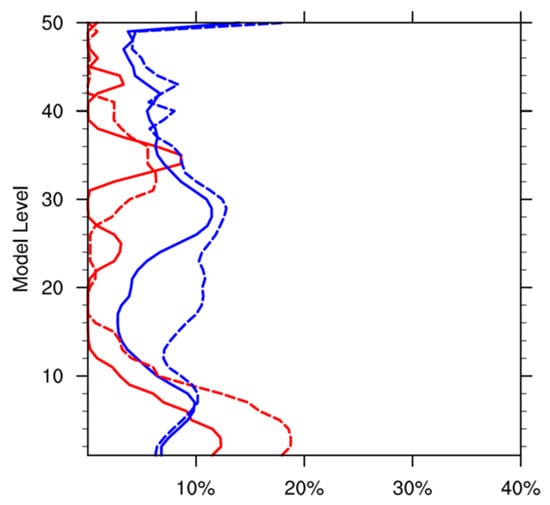
Figure 1. Contribution of the balanced part of T (blue) and χ (red) to their full field in the CV5 BE of the TC season (solid lines) and winter (dashed lines).

Figure 2a–f compare the contributions of the balanced part in the CV6 BE between the TC season and winter. The balanced part of T with ψ (blue lines in Figure 2a,b) has a structure identical to that in the CV5 BE. The balanced part of T with χ_u (the last term in Equation (4)), which reflects the coupling between divergent wind and T, shows a marked seasonal difference below the tropopause. Its larger magnitude during the TC season (red lines in Figure 2a,b) suggests a stronger thermal influence on divergent wind in the weather systems of TC season.

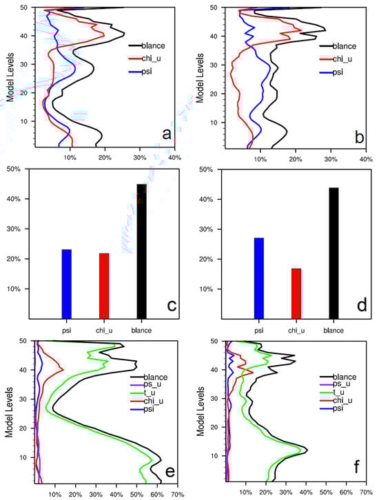
Figure 2. Contribution of the balanced parts to their full fields for T (a,b), Ps (c,d) and rhs (e,f) in the CV6 BE of the TC season (left) and winter (right). The black lines denote the total balanced parts, and the colored lines represent the constituent parts given by Equations (4)–(6).

For Ps, the total contribution of balanced parts (black columns in Figure 2c,d) is generally comparable between the TC season and winter. However, the balanced part with χ_u (red columns) is nearly as large as that with ψ (blue columns) during the TC season, whereas in winter it is only about half. This implies a stronger coupling between the mass field and divergent wind in the TC season.

A key feature distinguishing the CV6 scheme is its treatment of moisture (Equation (6)). The total contribution of balanced parts of rhs (black lines in Figure 2e,f) is dominated by the balanced part with T (green lines) in both seasons. The contributions of balanced part with momentum variables or Ps are small. Nevertheless, notable seasonal differences exist, for example, in winter, the strongest coupling between rhs and T occurs near 850 hPa and weakens rapidly downward. In contrast, during the TC season, this coupling is considerably stronger and extends from 850 hPa down to the surface.

3.2. The First Eigenvectors

The average vertical autocorrelations of the CVs are modeled via empirical orthogonal function (EOF) decomposition, with the first eigenvector representing the dominant vertical mode.

In the CV5 BE, the primary seasonal difference in this mode manifests in χ_u and rhs. For χ_u, an oscillatory structure is observed (Figure 3a), consistent with the constraint of near-zero total column divergence. During the TC season, a negative correlation is evident between 700 hPa and 300 hPa (Table 2), a feature absent in winter. This contrast suggests the presence of more intense lower-level convergence coupled with upper-level divergence within TC-season convective systems. As for rhs, both seasons exhibit a monotonic vertical correlation (Figure 3b); however, the extremum is located at a higher altitude during the TC season, indicating deeper vertical development of convective systems. Analogous characteristics are observed in the CV6 BE. Similarly, in the CV7 BE, the first eigenvectors of U and V resemble that of rhs in the CV5 BE, with the extremum also located higher in the TC season (Figure 3c,d).

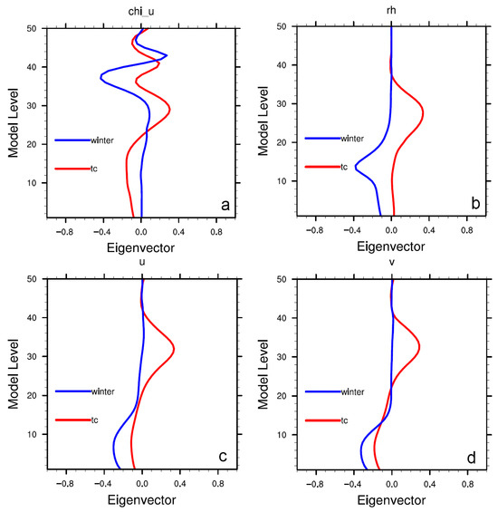
Figure 3. The first eigenvectors for χ_u (a), rhs (b) in the CV5 BE, and for U (c), V (d) in the CV7 BE of the TC season (red lines) and winter (blue lines).

3.3. The Horizontal Length Scales

The horizontal length scale quantifies the horizontal autocorrelation for each vertical EOF mode of the CVs, representing the horizontal influence radius of observations. They are generally smaller in the TC season than in winter for most modes (Figure 4), suggesting that weather systems during TC season exhibit smaller-scale characteristics. While the CV5 BE shows horizontal length scales below 80 km for T_u and rhs but near 500 km for ψ and χ_u (Figure 4a–d), the CV7 BE reduces momentum CV horizontal length scales to a magnitude similar to those of T_u (Figure 4e,f). This demonstrates that the CV7 BE better captures small-scale momentum error structures, confining increments closer to observations and thereby enhancing its utility for convective-scale prediction in high-resolution DA, such as in radar radial velocity DA [8] and wind profiler DA [9].

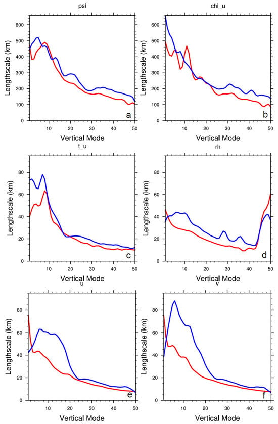
Figure 4. Horizontal length scales for ψ (a), χ_u (b), T_u (c) and rhs (d) in the CV5 BE, and for U (e), V (f) in the CV7 BE of the TC season (red lines) and winter (blue lines).

3.4. Single Pseudo-Observation Tests

The single pseudo-observation test is an effective method to illustrate how the differences in the statistical properties of BE affect the analysis field differently through an isolated observation. One test assimilates a pseudo-T observation with the CV5 BE. This observation is placed at the center of the model domain on the 18th level, where the contribution of the balanced part of T with ψ shows the greatest seasonal difference (blue lines in Figure 1). Analysis increments at this level (Figure 5) demonstrate that the TC season BE yields weaker and more confined wind increments than winter BE, despite an identical T observation being assimilated. This result stems from both the weaker T–momentum coupling and the shorter horizontal length scales in the TC season BE (Figure 4a–d). Similarly, the wind increments propagate over much larger distances than the T increments because ψ and χ_u are employed as momentum CVs.

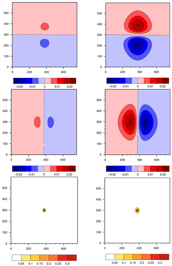
Figure 5. Horizontal cross section of the resulting increments of U, V (m s⁻¹) and T (K) (from top to bottom) in the pseudo-observation test of T (innovation of 1 K) using the CV5 BE of the TC season (left) and winter (right).

The assimilation of a pseudo-T observation at the 4th model level using the CV6 BE produces non-zero moisture increments via multivariate analysis of moisture in this scheme. The stronger T–moisture coupling and the shorter horizontal length scales in the TC season BE leads to larger but less extensive increments compared to winter, as indicated in Figure 6.

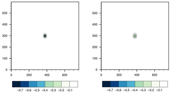
Figure 6. Horizontal cross section of the resulting increments of water vapor mixing ratio (g kg⁻¹) in the pseudo-observation test of T (innovation of 1 K) using the CV6 BE of the TC season (left) and winter (right).

When a pseudo-U observation at the 32nd model level is assimilated, the use of CV7 BE results in a much smaller influence radius for the wind observation, whereas the momentum increments display a larger gradient, compared to the CV5 BE (Figure 7a,b). Additionally, the TC season BE produces a stronger vertical spread of momentum increments in the upper troposphere relative to the winter BE (Figure 7c,d), a result consistent with the features of the first eigenvector in Figure 3c.

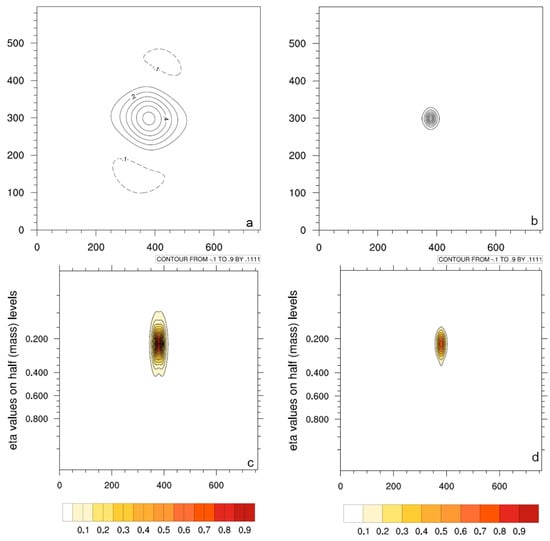
Figure 7. Horizontal cross section of the resulting U increments (m s⁻¹) using the CV5 BE (a) and the CV7 BE (b) of the TC season and the vertical cross section using the CV7 BE of the TC season (c) and winter (d) in the pseudo-observation test of U (innovation of 1 m s⁻¹).

4. Impact on TC Track Forecasts with Real DA

4.1. Model Configuration and Experimental Design

WRFDA [16] version 3.8 is used in this study based on its recognized code stability and reliability. And to maintain compatibility with the WRFDA, WRF [13] version 3.8 is correspondingly used. The simulation employs a single domain centered at 30°N and 120°E, with dimensions of 760 × 600 grid points and a horizontal grid spacing of 9 km. The model configuration includes 51 vertical levels, extending up to 10 hPa, and a time step of 45 s. Key physics parameterizations consist of the Thompson microphysics scheme [17], the Rapid Radiative Transfer Model for Global Climate Models (RRTMG) [18] longwave and shortwave schemes, and the Yonsei University (YSU) boundary layer parameterization [19]. Cumulus parameterization is turned off. For direct satellite DA, the Community Radiative Transfer Model (CRTM) [20] version 2.1.3 is employed as the observation operator, with a 3 h assimilation window.

In the ranking of the ten least accurate official track forecasts by the China Meteorological Administration (CMA) at 24, 48, and 72 h lead times in 2018, fourteen forecasts related to four TCs are identified, with their entire 72 h observed tracks falling within the domain of our TC forecasting system. This study is conducted based on these 14 cases (Table 3), which comprise four forecasts for TC Jelawat (1803), three for TC Prapiroon (1807), four for TC Jebi (1812), and three for TC Yagi (1814).

Table 3. Names of the TCs (in 2018), the initial time (mmddhh in UTC, where mm is two-digit month, dd is day of the month, and hh is hour) of the forecast, and the official forecast error (km) from CMA.

TC	Initial Time	24 h	48 h	72 h
Jelawat	032700			449
Jelawat	032800			448
Jelawat	032812			464
Jelawat	032818			537
Prapiroon	062900			559
Prapiroon	062906			474
Prapiroon	062912			526
Jongdari	072806		393
Jongdari	072812		452
Jongdari	072818		552
Jongdari	072900		412
Yagi	080900			539
Yagi	080906	222	363	503
Yagi	081000		356

For each case, one control experiment (CTRL) and three DA experiments are conducted. The DA experiments employed the CV5, CV6 and CV7 BEs of the TC season, respectively. For the DA experiments, the background field is obtained by interpolating the National Centers for Environmental Prediction (NCEP) global forecast system (GFS) 6 h forecast valid at the initial time. The CTRL uses this interpolated field directly as its initial condition. Lateral boundary conditions for all experiments are provided by the GFS forecasts.

4.2. Observational Data

In addition to conventional observations, the assimilated data comprise satellite brightness temperature data from microwave sounders and a single real-time minimum sea level pressure (MSLP) observation provided by the CMA. The observation errors provided with WRFDA version 3.8 for each observation type are used in this study.

Conventional data sourced from the Global Telecommunications System (GTS) include radiosonde observations (TEMP), atmospheric motion vectors (AMV), aerodrome routine meteorological reports (METAR), automated aircraft reports (AMDAR), satellite remote upper-air soundings (SATEM), upper-wind reports (PILOT), and space-based GPS radio occultation (GPSRO) data. Figure 8a illustrates the distribution of AMVs between 200 and 300 hPa assimilated in the forecast initialized at 12 UTC on 28 March, while Figure 8b displays the corresponding distribution of radiosonde observations.

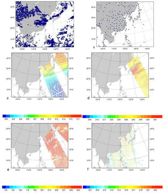
Figure 8. The distribution of atmospheric motion vectors between 200 and 300 hPa (a), radiosonde (b), brightness temperature from METOP-B AMSU-A channel 9 (c) and METOP-A MHS channel 3 (d) used in forecast 032812 and brightness temperature from NOAA-19 MHS channel 4 (e) and JPSS ATMS channel 9 (f) used in forecast 080906.

The microwave brightness temperature data assimilated in this study are obtained from the Advanced Microwave Sounding Unit-A (AMSU-A), the Microwave Humidity Sounder (MHS), and the Advanced Technology Microwave Sounder (ATMS). These instruments are widely acknowledged as major contributors to the skill of contemporary numerical weather prediction [21]. Only clear-sky radiances over ocean surfaces are assimilated using a 120 km thinning grid. Due to the model top being set at 10 hPa, channels with weighting functions peaking above channel 9 for AMSU-A and above channel 10 for ATMS are excluded. Surface-sensitive channels are also omitted. A detailed summary of the satellite microwave brightness temperature data used is provided in Table 4. Biases in these observations are mitigated using the Variational Bias Correction (VarBC) scheme [22]. Collectively, these observations offer extensive spatial coverage over the ocean within the assimilation window (Figure 8c–f).

Table 4. The microwave brightness temperature data used in this study.

Sensor	Platform	Channels Used
AMSU-A	NOAA-15	5, 7~9
	NOAA-18	6, 7
	NOAA-19	5, 6, 9
	METOP-A	5, 6, 9
	METOP-B	8~9
	AQUA	6, 8~9
MHS	NOAA-19	4~5
	METOP-A	3~5
	METOP-B	3~5
ATMS	JPSS	6~10, 18~19

Despite the growing abundance of satellite and radar observations, accurately initializing the true structure of TCs and their surrounding environment remains a persistent challenge [23]. A widely used approach to address this issue is DA, which integrates TC observations and/or a bogus vortex to improve the initial analysis [24]. In line with Kleist [25] and Lim et al. [26], this study assimilates a single MSLP observation simultaneously with other observations, rather than employing a bogus vortex to pre-adjust the TC structure, in order to more effectively utilize the satellite data.

4.3. Test Results and Analysis

4.3.1. One Case Study

The forecast for TC Yagi initialized at 0600 UTC 9 August 2018 is the only case to exhibit consistently large official track errors across all three lead times (24, 48, and 72 h; Table 3). Therefore, this case is selected to illustrate the impact of the BE on the analysis and forecast of TC structure and track. Since the average results indicate that the CV5 experiment does not achieve the best performance at any forecast lead time among the three BEs (shown in Section 4.3.2), we focus our discussion on the CV6 and CV7 experiments in this section.

Regarding track prediction (Figure 9a), among the three DA tests, the CV7 experiment most closely resembles CTRL, with the primary forecast adjustments occurring within the first 24 h. The CV6 experiment produces a track that agrees most closely with the observations. Notably, it best captures the southward recurvature between 48 h and 54 h (from 25.3°N to 24.9°N), whereas the TC in the CV7 experiment continues moving northwest during this period (from 25.1°N to 25.9°N). A comparison between the two DA experiments (Figure 9c,d) shows that the 48 h forecast of large-scale environmental flow in the CV6 experiment is more favorable for TC recurvature. In this experiment, the deep-layer mean (850–500 hPa) wind west of the TC center exhibits a stronger southward component. This steering flow pattern is in better agreement with the corresponding GFS analysis (Figure 9b). Furthermore, although the subtropical high is weaker in both DA experiments than in the GFS analysis, it remains relatively stronger in the CV6 run, with its western edge extending westward beyond 135°E, in contrast to the CV7 experiment.

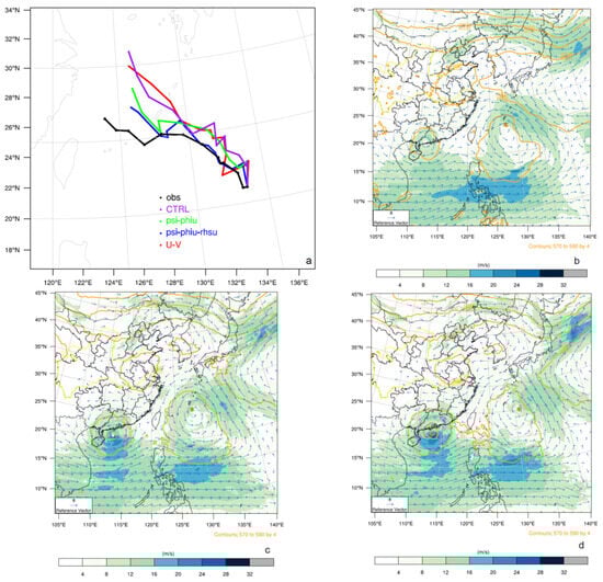
Figure 9. 72 h track forecast initialized at 0600 UTC 9 August for TC Yagi (a), GFS analysis of geopotential height (gpm) at 500 hPa (orange contours) and 850-500 hPa layer-mean wind field (shading and vectors) at 0600 UTC 11 August (b) and 48 h forecast (valid at 0600 UTC 11 August) of the same fields from the CV6 test (c) and CV7 test (d). The symbol “*” denotes the forecasted TC center position.

Figure 10 illustrates the differences in the horizontal distribution of the analysis increments (differences between analysis and background) from the two DA experiments. In contrast to the CV7 experiment, which exhibits only a slight decrease in SLP near the TC center (Figure 10b), the CV6 experiment shows an east-high, west-low SLP increment pattern (Figure 10a). The 500 hPa wind increments are consistent with these pressure increments: the CV6 experiment is characterized by westerly wind increments, whereas the CV7 experiment shows only very weak cyclonic circulation increments near the TC center (Figure 10c,d). The combined effect of these pressure and wind increments in the CV6 experiment appears to promote the westward movement of TC Yagi. The 6 h forecasted longitudinal position shifts from 133.8°E in the CTRL run to 133.5°E, moving closer to the observed position of 133.3°E. By contrast, the absence of such increments in the CV7 experiment likely hinders a comparable westward adjustment in its 6 h forecast, which remains at 133.9°E. The analysis increments of 700 hPa water vapor mixing ratio and 300 hPa temperature exhibit comparable spatial patterns yet differ in magnitude between the CV6 and CV7 experiments. The CV6 experiment generates an initial structure with a moister lower layer and a warmer upper layer (Figure 10e–h). This configuration favors the subsequent development of a more organized TC vortex after six hours, as evidenced by intensified tangential winds and a warmer, moister core in the lower troposphere (Figure 11). It is also worth noting that although the positive temperature anomalies near 200 hPa appear relatively weak, a closer inspection reveals the emergence of a stronger warm anomaly at 300 hPa in CV6 than in CV7, despite its still limited spatial extent.

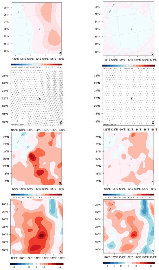
Figure 10. Horizontal distribution of the analysis increments of SLP (hPa, (a,b)), wind vector at 500 hPa (m s⁻¹, (c,d)), water vapor mixing ratio at 700 hPa (g kg⁻¹, (e,f)) and temperature at 300 hPa (K, (g,h)) in experiments CV6 (left) and CV7 (right) for TC Yagi initialized at 0600 UTC 9 August. Symbol “*” denotes the observed TC center position.

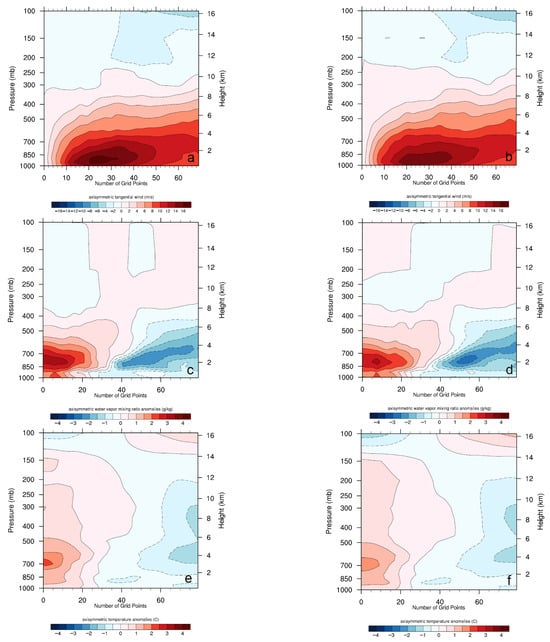
Figure 11. Vertical cross section of axisymmetric mean of 6 h forecast of tangential wind (m s⁻¹, (a,b)), water vapor mixing ratio deviation (g kg⁻¹, (c,d)) and temperature deviation (K, (e,f)) in experiments CV6 (left) and CV7 (right) for TC Yagi initialized at 0600 UTC 9 August. X-axis is the number of grid point relative to the TC center.

4.3.2. Comparisons for All Cases

The mean track errors for the 14 cases (Figure 12) indicate that DA with any of the three BEs improves TC track forecasts compared to the CTRL. However, the degree of improvement varies depending on the BE used. The CV7 BE yields the most pronounced enhancement in the 24 h forecasts, reducing the mean track error from 97 km in CTRL to 69 km, whereas the CV6 BE results in an error of 80 km. At longer lead times, the CV6 BE demonstrates a more considerable advantage. It reduces the mean 48 h error from 244 km to 174 km and the 72 h error from 374 km to 285 km. In comparison, the errors in the CV7 experiment are reduced only to 210 km and 327 km, respectively. The CV5 BE does not achieve the best performance at any forecast lead time among the three BEs. However, as the lead time increases, its improvement relative to the CV7 BE becomes progressively more apparent.

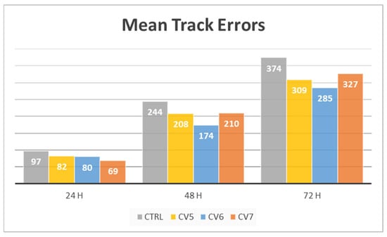
Figure 12. Mean track errors (km) of 14 forecasts.

These results can be attributed to the distinct structural characteristics of each BE, as discussed previously. The momentum CV scheme in the CV7 BE more effectively captures small-scale features of momentum error, leading to greater forecast improvements at shorter lead times. In contrast, the CV6 BE incorporates more information regarding large-scale momentum errors, which contributes to better refinement of the environmental field at synoptic scales. Moreover, unlike the univariate analysis in the CV7 BE, the multi-variate couplings in the CV6 BE, such as wind-temperature and wind-pressure covariances, allow observational information from satellite microwave brightness temperatures to be used in a dynamically consistent manner. This synergistic effect results in closer fits to the satellite microwave brightness temperature data, as reflected in the lower RMS of the observation-minus-analysis (OMA) across all channels in the CV6 experiment compared to the CV7 experiment (Figure 13). Such improvement is particularly important for forecasting TCs, which often develop over data-sparse oceanic regions. The combined effect of improved environmental representation and physically consistent data assimilation gives the CV6 BE superior forecast skill at longer lead times. Meanwhile, the CV5 BE, with its more limited multivariate coupling, attains an intermediate level of performance between CV6 and CV7 as the forecast range extends.

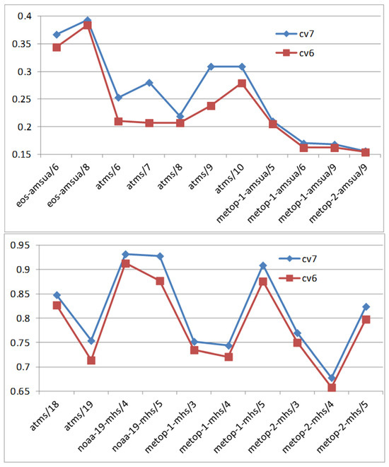
Figure 13. Comparison of the RMS of brightness temperature observation minus analysis (OMA) of each channel in forecast 032812 and 080906 between the CV6 experiment and the CV7 experiment.

In this study, TC intensity forecasts from our TC forecasting system demonstrate lower sensitivity to BE than track forecasts (Table 5). Among the DA experiments, the maximum difference in maximum 10 m wind speed errors is 1.5 m s⁻¹, as evidenced by the 48 h errors ranging from 7.4 m s⁻¹ to 8.9 m s⁻¹. Similarly, the minimum sea level pressure errors differ by no more than 1 hPa across the experiments, exemplified by the 72 h errors ranging from 12.6 hPa to 13.6 hPa.

Table 5. Mean intensity errors of 14 forecasts.

	Maximum 10 m Wind Error (m s−1)				MSLP Error (hPa)
	CTRL	CV5	CV6	CV7	CTRL	CV5	CV6	CV7
24 h	4.5	4.2	3.9	4.3	5.2	4.9	4.2	5.1
48 h	9.2	8.8	7.4	8.9	16.4	13.7	13.7	14.4
72 h	7.7	7.5	6.6	7.6	13.8	13.0	12.6	13.6

5. Discussion

Considering the potential uncertainties in current TC intensity analysis, the preliminary results from these 14 forecasts do not indicate a distinct advantage of any specific BE scheme for TC intensity forecasting. It is noteworthy that the satellite microwave brightness temperature data is assimilated after thinning, and the 9 km model resolution is relatively coarse. Both factors may somewhat constrain the full potential of the CV7 BE. Further study is still needed to assess the impact of BE on TC forecasting using DA system and forecast model with higher resolution and finer physical parameterization schemes. One more challenging issue that needs to be studied is to improve BE to be more suitable for all-sky radiance DA, which should be crucial to improve TC intensity and precipitation forecast. The BEs in this study still have limitations in TC regions characterized by dominant small-scale features and prominent convective activity. On one hand, the BE for the TC inner-core region could be specifically estimated; on the other hand, introducing flow-dependent ensemble-based BE may help to compensate for these limitations.

6. Conclusions

In this study, we developed and evaluated BEs for a TC forecasting system over the western North Pacific. A total of six BEs were modeled using three CV schemes with training data from two periods corresponding to the TC season and the winter season, respectively.

Since TCs exhibit distinct characteristics compared to other weather systems, the structural features of BEs modeled with training data from the TC season and the winter season are first compared. In the TC season, the correlation between the non-divergent wind and the mass field is smaller, as well as the correlation between the non-divergent wind and the divergent wind. In contrast, the correlation between the divergent wind and the mass field is larger, as is the correlation between the temperature and the humidity. The horizontal length scale of each CV is generally smaller. The first eigenvector of the unbalanced velocity potential and humidity in the TC season is also significantly different from winter. These features indicate that in the TC season the systems have a statistically smaller horizontal scale, deeper vertical development, and stronger divergence at high levels. The thermal effect also has a stronger influence on the divergence field than in winter. These structural differences demonstrate that BEs are sensitive to the seasonal characteristics of the training data, justifying the use of TC-season data for optimal BE estimation in TC forecasting. Pseudo single observation tests are then performed to show how the differences in the statistical properties of BE affect the field of analysis differently.

The performance of TC-season BEs derived from different CV schemes is then assessed for TC track forecasting through the assimilation of satellite brightness temperature data from microwave sounders. The evaluation is based on a set of 14 cases from 2018 that exhibited large official track errors. The results indicate that DA with any of the three BEs improves TC track forecasts compared to the CTRL. However, the degree of improvement varies depending on the BE used. The momentum CV scheme in the CV7 BE more effectively captures small-scale features of momentum error, leading to greater forecast improvements at shorter lead times, i.e., the 24 h mean track error is reduced from 97 km in the CTRL to 69 km. In contrast, the CV6 BE incorporates more information regarding large-scale momentum errors, which contributes to better refinement of the environmental field at synoptic scales. Furthermore, compared to the univariate analysis in the CV7 BE, the CV6 BE benefits from multivariate couplings, facilitating closer fits to satellite microwave brightness temperature data, which is particularly crucial for forecasting TCs that primarily develop over oceans where conventional observations are scarce. As a result, at longer lead times, the CV6 BE demonstrates a more considerable advantage. It reduces the mean 48 h error from 244 km to 174 km and the 72 h error from 374 km to 285 km. In comparison, the errors in the CV7 BE experiment are reduced only to 210 km and 327 km, respectively. The CV5 BE does not achieve the best performance at any forecast lead time among the three BEs. However, as the lead time increases, its improvement relative to the CV7 BE becomes progressively more apparent.

References

- Lorenc, A.C. Modelling of error covariances by 4D-Var data assimilation. Q. J. R. Meteorol. Soc. 2003, 129, 3167–3182. [Google Scholar] [CrossRef]
- Sasaki, Y. Some basic formalisms in numerical variational analysis. Mon. Wea. Rev. 1970, 98, 875–883. [Google Scholar] [CrossRef]
- Evensen, G. Sequential data assimilation with a nonlinear quasi-geostrophic model using Monte Carlo methods to forecast error statistics. J. Geophys. Res. Ocean 1994, 99, 10143–10162. [Google Scholar] [CrossRef]
- Rabier, F.; Jrvinen, H.; Klinker, E.; Mahfouf, J.F.; Simmons, A. The ECMWF operational implementation of four-dimensional variational assimilation. I: Experimental results with simplified physics. Q. J. R. Meteorol. Soc. 2000, 126, 1143–1170. [Google Scholar] [CrossRef]
- Hamill, T.M.; Snyder, C. A hybrid ensemble Kalman filter–3D variational analysis scheme. Mon. Wea. Rev. 2000, 128, 2905–2919. [Google Scholar] [CrossRef]
- Chen, Y.D.; Xia, X.; Min, J.Z.; Huang, X.Y.; Rizvi, S.R. Balance characteristics of multivariate background error covariance for rainy and dry seasons and their impact on precipitation forecasts of two rainfall events. Meteorol. Atmos. Phy. 2016, 128, 579–600. [Google Scholar] [CrossRef]
- Gao, X.; Gao, S. Impact of Multivariate Background Error Covariance on the WRF-3DVAR Assimilation for the Yellow Sea Fog Modeling. Adv. Meteorol. 2020, 2020, 8816185. [Google Scholar] [CrossRef]
- Sun, J.; Wang, H.; Tong, W.; Zhang, Y.; Lin, C.-Y.; Xu, D. Comparison of the Impacts of Momentum Control Variables on High-Resolution Variational Data Assimilation and Precipitation Forecasting. Mon. Wea. Rev. 2016, 144, 149–169. [Google Scholar] [CrossRef]
- Wang, C.; Chen, Y.; Chen, M.; Shen, J. Data assimilation of a dense wind profiler network and its impact on convective forecasting. Atmos. Res. 2020, 238, 104880. [Google Scholar] [CrossRef]
- Chen, Y.D.; Rizvi, S.R.; Huang, X.Y.; Min, J.; Zhang, X. Balance characteristics of multivariate background error covariances and their impact on analyses and forecasts in tropical and Arctic regions. Meteorol. Atmos. Phy. 2013, 121, 79–98. [Google Scholar] [CrossRef]
- Wang, R.C.; Gong, J.D. Review of Dynamic Balance Constraints Construction Using Background Error Covariance in Variational Assimilation Schemes. Meteorol. Mon. 2016, 42, 1033–1044. (In Chinese) [Google Scholar]
- Lee, J.; Huang, X.Y. Background error statistics in the Tropics: Structures and impact in a convective-scale numerical weather prediction system. Q. J. R. Meteorol. Soc. 2020, 146, 2154–2173. [Google Scholar] [CrossRef]
- Skamarock, W.; Klemp, J.; Dudhia, J.; Gill, D.O.; Barker, D.M.; Duda, M.G.; Huang, X.-Y.; Wang, W.; Powers, J.G. A Description of the Advanced Research WRF, Version 3; NCAR Tech. Note NCAR/TN-475_STR: Boulder, CO, USA, 2008; p. 125. [Google Scholar]
- Wang, H.; Huang, X.Y.; Sun, J. A comparison between the 3/4DVAR and hybrid ensemble-VAR techniques for radar data assimilation. In Proceedings of the 36th Conference on Radar Meteorology, Breckenridge, CO, USA, 16–20 September 2013; Available online: https://api.semanticscholar.org/CorpusID:126172409 (accessed on 10 June 2025).
- Parrish, D.F.; Derber, J.C. The national meteorological center’s spectral statistical-interpolation analysis system. Mon. Wea. Rev. 1992, 120, 1747–1763. [Google Scholar] [CrossRef]
- Barker, D.; Huang, X.Y.; Liu, Z.; Auligné, T.; Zhang, X.; Rugg, S.; Ajjaji, R.; Bourgeois, A.; Bray, J.; Chen, Y.; et al. The weather research and forecasting model’s community variational/ensemble data assimilation system: Wrfda. Bull. Amer. Meteor. Soc. 2012, 93, 831–843. [Google Scholar] [CrossRef]
- Thompson, G.; Field, P.R.; Rasmussen, R.M.; Hall, W.D. Explicit forecasts of winter precipitation using an improved bulk microphysics scheme. Part II: Implementation of a new snow parameterization. Mon. Wea. Rev. 2008, 136, 5095–5115. [Google Scholar] [CrossRef]
- Mlawer, E.J.; Taubman, S.J.; Brown, P.D.; Iacono, M.J.; Clough, S.A. Variational data assimilation with an adiabatic version of the NMC spectral model. Mon. Wea. Rev. 1997, 102, 16663–16682. [Google Scholar]
- Hong, S.-Y.; Noh, Y.; Dudhia, J. A revised approach to ice microphysical processes for the bulk parameterization of clouds and precipitation. Mon. Wea. Rev. 2006, 132, 2318–2341. [Google Scholar] [CrossRef]
- Weng, F. Advances in radiative transfer modeling in support of satellite data assimilation. J. Atmos. Sci. 2007, 64, 3799–3807. [Google Scholar] [CrossRef]
- Eyre, J. Impact studies with satellite observations at the Met Office. In Proceedings of the Fifth WMO Workshop on the Impact of Various Observing Systems on Numerical Weather Prediction, Sedona, AZ, USA, 22–25 May 2012; WMO: Geneva, Switzerland, 2012. [Google Scholar]
- Dee, D.P.; Uppala, S. Variational bias correction of satellite radiance data in the ERA-Interim reanalysis. Q. J. R. Meteorol. Soc. 2009, 135, 1830–1841. [Google Scholar] [CrossRef]
- Torn, R.D. Performance of a mesoscale ensemble Kalman filter (EnKF) during the NOAA high-resolution hurricane test. Mon. Wea. Rev. 2010, 138, 4375–4392. [Google Scholar] [CrossRef]
- Wang, M.; Xue, M.; Zhao, K.; Dong, J. Assimilation of T-TREC-retrieved winds from single-Doppler radar with an ensemble Kalman filter for the forecast of Typhoon Jangmi (2008). Mon. Wea. Rev. 2014, 142, 1892–1907. [Google Scholar] [CrossRef]
- Kleist, D.T. Assimilation of tropical cyclone advisory minimum sea level pressure in the NCEP global data assimilation system. Wea. Forecast. 2011, 26, 1085–1091. [Google Scholar] [CrossRef][Green Version]
- Lim, S.; Song, H.J.; Kwon, I.H. A Tropical Cyclone Initialization in Multi-Scale Localization with Hybrid Four Dimensional Ensemble-Variational System: Preliminary Results. SOLA 2020, 16, 145–150. [Google Scholar] [CrossRef]
Disclaimer/Publisher’s Note: The statements, opinions and data contained in all publications are solely those of the individual author(s) and contributor(s) and not of MDPI and/or the editor(s). MDPI and/or the editor(s) disclaim responsibility for any injury to people or property resulting from any ideas, methods, instructions or products referred to in the content. |
© 2026 by the authors. Licensee MDPI, Basel, Switzerland. This article is an open access article distributed under the terms and conditions of the Creative Commons Attribution (CC BY) license.