An Improved Closed-Form Multi-Baseline Phase Unwrapping Algorithm

Highlights

What are the main findings?

• The number of theoretical intercepts and the calculation method for each one are specified precisely.
• The practical intercept filtering method and the closed-form solution for ambiguity number are presented.

What is the implication of the main finding?

• The process of intercept search and ambiguity number search has been avoided. This has significantly enhanced processing efficiency.
• Constructing and solving the Chinese Remainder Theorem equations with error-free intercepts as remainders has greatly improved processing accuracy.

Abstract

Multi-baseline phase unwrapping (PU) is an extension of single-baseline PU. Its accuracy directly affects the reliability of results in engineering tasks, such as InSAR topographic mapping and geological hazard monitoring, in complex scenarios. Meanwhile, its efficiency determines the timeliness of data delivery in emergency scenarios. The cluster-analysis (CA)-based algorithm represents a significant advancement in multi-baseline PU algorithms, wherein a strategy for pixel clustering and uniform PU is introduced. However, in the CA algorithm, phase noise degrades pixel clustering performance, leading to deviations in the determination of intercept centerlines and ultimately errors in ambiguity number search. In addition, the computational complexity is increased by the search for intercept peaks and ambiguity numbers. To address these limitations and ensure that accuracy and efficiency requirements are met in practical applications, an improved closed-form multi-baseline PU algorithm is proposed in this article. Compared with conventional CA algorithms, this algorithm offers the following four improvements. First, differential phase processing is introduced into the algorithm, which not only mitigates the impact of phase noise on pixel clustering but also provides new inputs for subsequent ambiguity-number solution. Secondly, a novel method for calculating the theoretical intercept is proposed, which depends solely on the external reference DEM and the ambiguity height. Thirdly, to eliminate the need for peak-intercept search and to suppress error propagation from incorrect intercepts, an intercept filtering method is introduced into the algorithm. In this method, a categorized filtering of actual intercepts for all pixels is performed. Fourthly, to address the phase-noise sensitivity and low efficiency in ambiguity-number search, the algorithm proposes a closed-form ambiguity-number solution method based on the Chinese Remainder Theorem (CRT). In this method, calculation accuracy can be ensured and solution efficiency improved by constructing and solving CRT equation groups with filtered error-free intercepts as remainders. The aforementioned four points are not independent of each other, but are strongly logically dependent and correlated. The effectiveness of the proposed algorithm is validated through one simulated data experiment and two real data experiments. The proposed algorithm achieves improvements in accuracy and efficiency across the three datasets. In terms of accuracy, the RMSE is reduced by at least 11.52%, while the PUSR increases by at least 1.36%. In terms of efficiency, runtime is shortened by at least 29.75%.

1. Introduction

Interferometric synthetic aperture radar (InSAR) is a key technology for measuring surface elevation and monitoring topographic changes. The InSAR technique is capable of all-day, all-weather, wide-area observations, enabling efficient generation of high-resolution digital elevation models (DEMs). Its advantages make it particularly valuable in areas where traditional measurement methods are not effective [1,2,3]. InSAR has become an important technological approach in scientific research and engineering practice related to Earth mapping, disaster monitoring and assessment, natural resource exploration, and geographic information [4,5,6,7]. InSAR utilizes two coherent synthetic aperture radar(SAR) images of the same target area to perform interferometric processing, which produces interferometric phase information. Since the interferometric phase ranges from [$-\pi$, +$\pi$), PU is required to recover the true phase. The surface elevation is then derived through the phase-to-height conversion process [8]. In conventional single-baseline InSAR processing, the same interferometric phase combined with different ambiguity numbers results in different absolute phases, indicating that PU is an ill-posed problem [9,10]. To obtain a unique absolute phase from the interferometric phase, it needs satisfying the phase continuity assumption, which requires the phase gradient between adjacent pixels to be less than $\pi$ [11,12]. However, this assumption often becomes invalid under complex topographic conditions (e.g., mountainous areas, steep slopes, and cliffs), substantially reducing the performance of conventional single-baseline PU methods.

Since the 1990s, multi-baseline PU technology has advanced significantly. In [13], three methods inculding CRT, projection method and linear combination method, were proposed to process multi-baseline, multi-frequency InSAR data, while analyzing their error characteristics. In [14], a three-antenna SAR interferometric system was introduced to acquire phase and amplitude information, and the ambiguity height was extended by combining different baselines. In [15], a multi-frequency InSAR PU algorithm based on the maximum likelihood estimation (MLE) was proposed, which ensures the uniqueness of the solution in phase discontinuity regions. The drawback of the MLE multi-frequency method is that it requires a large number of interferograms to ensure good performance. Compared with the number of interferograms required by the aforementioned MLE algorithm to obtain reliable height estimates, the subsequent maximum a posteriori (MAP) method can reduce the number of interferograms. In [16,17], a MAP estimation method based on Markov Random Field (MRF) was introduced. This method incorporates prior statistical information via the MRF model and estimates height values by optimizing its hyperparameters. However, the aforementioned algorithm struggles to accurately reconstruct the true interferometric phase when the quality of the interferogram is severely compromised due to large registration errors. Consequently, in [18], a method was proposed to estimate interferometric phase under significant registration errors. This method employs coherence information between adjacent pixel pairs to automatically register SAR images and exploits the orthogonality of the signal and noise subspaces to suppress interferometric phase noise. In [19], two methods were proposed to solve layover based on multi-baseline InSAR technology using a wideband array model: one using terrain search and the other using joint range-pixel processing. In [20,21], effective CRT-based solution algorithms for multi-baseline data processing were introduced. To apply the improved robust closed-form CRT in multi-channel InSAR ground elevation profile reconstruction, in [22], a closed-form robust multi-baseline PU algorithm was introduced. This algorithm proposes an elevation reconstruction method based on the statistical characteristics of interferometric phases and combined interferogram information, employing a specialised weighted mean filtering technique to enhance the robustness of elevation reconstruction. In [23], the framework and key concepts of single-baseline PU were extended to multi-baseline PU, and a two-stage programming approach was proposed, demonstrating the potential of extending the most representative single-baseline PU methods to multi-baseline PU. In [24], a refined pure integer programming (RPIP)-based multi-baseline PU method by incorporating interferometric phase statistics was proposed. In [25], a refined two-stage programming approach (R-TSPA) was developed that effectively addresses the limitations of conventional two-stage programming approaches (TSPAs) while improving the processing accuracy. In [26], a robust redundant residue system (RRNS) was proposed to determine terrain height profiles with high precision, and the proposed algorithm can be generalized to real-world scenarios. In recent years, deep learning has also made significant strides in the field of multi-baseline PU. In [27], an unsupervised deep convolutional network (CANet) was proposed. This approach integrates ‘intercepts and interference fringes’ as input features (the ‘intercept-fringe pattern’), enabling rapid pixel grouping via a fully unsupervised self-training strategy. In [28], a novel and effective loss function was introduced by combining the contrast and structure scores from MS-SSIM with a relative difference loss. Previous multi-baseline InSAR deep learning research suffered from poor method comparability due to the ‘lack of unified datasets’. In [29], a large-scale benchmark dataset was constructed to address this issue. With the help of this dataset, deep convolutional neural networks (DCNNs) were thoroughly explored and tested.

CA-based multi-baseline PU algorithms represent a significant advancement in the field by shifting the focus from individual pixels to cluster groups. In [30], a CA-based multi-baseline InSAR PU algorithm was proposed, which clusters pixels with identical ambiguity number vector based on their intercepts. A search-based approach is then used to determine ambiguity numbers for each cluster group. In [31], the intercept dimension of the cluster algorithm was extended to row, line and intercept, and a CA-based noise-robust PU algorithm for multi-baseline interferograms (CANOPUS) was proposed to enhance performance under noisy conditions. In [32], a linear phase combination method was introduced to mitigate noise effects on cluster accuracy. In [33], a closed-form CA-based multi-baseline PU algorithm was proposed. This algorithm provides a closed-form solution for ambiguity number vectors and enhances robustness by filtering interferometric phases and optimizing baseline relationships. In [34,35], two cluster correction methods and the Block Matching and 3D Filtering (BM3D) algorithm were introduced into the cluster process, significantly improving noise robustness. In the deep learning era, the continued improvement of conventional CA algorithms stems from their complementary and irreplaceable practical advantages. Based on the geometric and physical principles of InSAR, these algorithms offer clear interpretability, meeting the demands of traceability and reliability in precision-sensitive tasks such as topographic mapping and deformation monitoring. They are lightweight and do not require large-scale labelled datasets or high-performance hardware. They also achieve phase unwrapping using geometric parameters and interferometric data alone, providing stability in scenarios where high-quality datasets are difficult to obtain. These traits enable improved CA algorithms to complement deep learning methods.

From a practical application perspective, tasks such as InSAR terrain mapping, geological disaster monitoring, and emergency terrain reconstruction have clear dual requirements for multi-baseline PU technology. On the one hand, it needs to ensure accuracy and reliability; on the other hand, it requires high computational timeliness. From the perspective of algorithm optimization, the conventional CA algorithm has shortcomings of being sensitive to phase noise and having high computational complexity, which makes it difficult to meet the needs of the aforementioned practical applications. Based on these two considerations, this paper proposes an improved closed-form multi-baseline PU algorithm. This algorithm not only meets the core requirements of accuracy and efficiency in practical applications but also reduces the CA algorithm’s sensitivity to phase noise while significantly improving its computational efficiency. The proposed algorithm differs from previous CA-based multi-baseline PU methods in four respects. First, differential phase processing is introduced, which extends the ambiguity height and provides new inputs for the subsequent ambiguity-number solution. Secondly, a new method for calculating theoretical intercepts has been established. This method integrates external reference DEM data for the observed area and ambiguity-height information, thereby yielding precise, finite theoretical intercepts. It is worth noting that the number of theoretical intercepts obtained here depends solely on the external reference DEM data of the observed area and ambiguity height information. Typically, this number is significantly fewer than the sum of the coprime numbers of the ambiguity heights minus one, as mentioned in [33]. Concurrently, this provides a reference basis for subsequent intercept filtering. Thirdly, an intercept filtering method is proposed to mitigate the impact of phase noise on intercept determination and eliminate the need for intercept search. Categorized filtering is then performed on the actual intercepts of all pixels. This method not only eliminates the computational overhead of intercept search but also ensures intercept accuracy. Fourthly, a closed-form ambiguity number solution method is proposed to reduce the influence of phase noise on ambiguity number determination and obviate the need for ambiguity number search. In this method, the reliability of PU results is ensured by constructing and solving CRT equation groups using filtered error-free intercepts as remainders.

The rest of this article is organized as follows. In Section 2, the geometric model of multi-baseline InSAR is introduced, and the advantages and limitations of the conventional CA algorithm are reviewed. A detailed description of the proposed algorithm is given in Section 3. The effectiveness of the proposed algorithm is validated through simulated and real data experiments in Section 4. The article is concluded in Section 5.

2. Analysis of Multi-Baseline InSAR and the CA Algorithm

Multi-baseline InSAR represents a significant advancement over traditional single-baseline InSAR. Multi-baseline InSAR systems typically employ two observational models: (1) simultaneous observations from multiple antennas, or (2) repeat-pass acquisition with different baseline configurations [36,37].

In the following, the geometric relationship of multi-baseline InSAR will be briefly introduced using simultaneous observation from multiple satellites as an example in Figure 1. Multiple satellites $S_1$, $S_2$, …, $S_N$ are distributed in a non-line-of-sight direction, forming multiple baselines. The projection of each baseline in the direction perpendicular to the line of sight is called the vertical effective baseline, denoted $B_1$, …, $B_{N-1}$, critical parameters within multi-baseline InSAR systems. $R_1$, $R_2$, …, $R_N$ represent the slant range between the antenna phase center of satellites $S_1$, $S_2$, …, $S_N$ and the ground observation point P. h is the terrain height of the ground observation point P. H is the height of the antenna phase center of the master satellite $S_1$. $\theta$ is the look angle of the master satellite $S_1$.

Figure 1. Geometric relationship of multi-baseline InSAR.

For simplicity, the following explanation uses the one-transmitter and two-receiver dual-baseline InSAR mode as an example. The flattened absolute phases corresponding to baselines $B_1$ and $B_2$ are ${\varphi }_1$ and ${\varphi }_2$, respectively, and their relationship to the height h of the target P is as follows:

$$\left\{\begin{array}{c}\hfill h={\displaystyle \frac{H_1{\varphi }_1}{2\pi }}\\ \hfill h={\displaystyle \frac{H_2{\varphi }_2}{2\pi }}\end{array}\right.$$

(1)

$H_1$ and $H_2$ are ambiguity heights corresponding to $B_1$ and $B_2$ respectively, representing a change in height when phase changes $2\pi$. The expression is as follows:

$$H_i={\displaystyle \frac{\lambda R_{1}sin\theta }{B_i}}$$

(2)

$\lambda$ is the wavelength of the signal. In practical processing, due to the limitations of trigonometric operations, the interferometric phases ${\phi }_1$ and ${\phi }_2$ obtained are wrapped phases of ${\varphi }_1$ and ${\varphi }_2$, with a range of [$-\pi ,\pi$). The relationship between them is as follows:

$${\phi }_i={\varphi }_i-2k_i\pi$$

(3)

$k_i$ is an ambiguity number, which is an integer. By combining (1) and (3), the following can be obtained as follows:

$$\left\{\begin{array}{c}\hfill h={\displaystyle \frac{H_1({\phi }_1+2k_1\pi )}{2\pi }}\\ \hfill ={\displaystyle \frac{H_2({\phi }_2+2k_2\pi )}{2\pi }}\end{array}\right.$$

(4)

Many conventional multi-baseline phase unwrapping algorithms require a pixel-by-pixel solution, resulting in high computational cost. The CA algorithm [30] proposed transforms (4) into a linear relationship between ambiguity numbers $k_1$ and $k_2$:

$$k_1={\displaystyle \frac{B_1}{B_2}}{k}_2+{\displaystyle \frac{B_1{\phi }_2-B_2{\phi }_1}{2\pi B_2}}$$

(5)

The slope term $B_1/B_2$ is a constant value, and the intercept term is as follows:

$$Inter={\displaystyle \frac{B_1{\phi }_2-B_2{\phi }_1}{2\pi B_2}}$$

(6)

$Inter$ is related to interferometric phases ${\phi }_1$ and ${\phi }_2$.

It can be inferred from (5) that pixels with identical intercepts correspond to exactly the same ambiguity number vector. Based on this principle, the CA algorithm groups pixels sharing the same intercept (i.e., the same ambiguity number vector) into an individual cluster group. In the subsequent process, the ambiguity number vector is computed on a cluster group rather than through pixel-wise calculation. The specific implementation steps of the CA algorithm are as follows (Algorithm 1). First, the actual intercept value for each pixel is calculated using (6). Second, a statistical histogram of the actual intercept values of all pixels is plotted, as shown in Figure 2, followed by cluster partitioning and peak searching on this histogram. Third, the intercept value corresponding to the centerline of each cluster group is adopted as the unified intercept value for all pixels within that cluster group. Fourth, each cluster group and its centerline intercept value are substituted into (5) to search for the corresponding ambiguity number vector [$k_1$, $k_2$]. Finally, substituting [$k_1$, $k_2$] into (3) yields the unwrapped phases. The above steps can be represented in pseudocode as follows. The core advantage of this algorithm is its ability to process all pixels within a cluster group as a single unit. Abandoning the pixel-wise independent operation mode significantly improves processing efficiency.

Algorithm 1 CA Algorithm

Input:  Parameters $\lambda$, R, $\theta$, $B_i$ and ${\phi }_i$ for i = 1, 2 Output:  Reconstructed unwrapped phase     1: Compute the actual intercept values $\widetilde{In}$ for all pixels via (6)     2: Perform statistical processing on $\widetilde{In}$     3: Perform clustering on all pixels based on intercept statistics     4: Perform peak search based on intercept statistics to obtain cluster centerlines     5: Assign the cluster centerline to each cluster group, respectively     6: for each cluster group do     7:    Search for [$k_1$, $k_2$] via (5)     8: end for     9: for each pixel do     10:    Obtain the ambiguity number by [$k_1$, $k_2$] of its corresponding cluster group     11:    Obtain ${\varphi }_i$ via (3)     12: end for     13: return Output

Figure 2. Qualitative description of intercept distributions at low and high noise levels. The dashed line depicts the distribution characteristics of the cluster group containing a small number of pixels under different noise levels. Under low-noise conditions, the cluster group exhibits a clear boundary, an intact structure, and no deviation of the cluster centerline. Under high-noise conditions, by contrast, its boundary becomes blurred, the cluster group tends to be absorbed by adjacent cluster groups, and the cluster centerline shifts significantly. (a) Intercept distribution under low noise level. (b) Intercept distribution under high noise level.

However, there are still some aspects in which the CA algorithm can be improved. It can be seen from (6) that intercepts are susceptible to phase noise. High phase noise can significantly disrupt the distribution of intercepts, causing issues such as the disappearance of cluster groups, blurred group boundaries, and deviated cluster centerlines. As illustrated in Figure 2a, under the condition of low phase noise, all cluster groups have intact structure, clear boundaries, and undeviated centerlines. In contrast, as the phase noise level increases, the distribution characteristics of the intercepts deteriorate markedly. As shown in the dashed-line area of Figure 2b, the originally well-defined cluster group becomes progressively blurred and absorbed by adjacent groups, directly leading to deviation of centerlines. The pixels corresponding to absorbed cluster groups are assigned incorrect centerlines. This leads to errors in the subsequent ambiguity-number search, resulting in incorrect unwrapping results. In addition, the computational complexity of the CA algorithm increases substantially due to searching for intercept centerlines and ambiguity numbers. The CA algorithm’s efficiency deteriorates significantly when dealing with large search spaces. In summary, the CA algorithm suffers from two major limitations: susceptibility to noise interference and computational inefficiency due to search operations.

3. Improved Closed-Form Multi-Baseline PU Algorithm

This section introduces an improved closed-form multi-baseline PU algorithm that addresses the limitations of the CA algorithm mentioned in Section 2. This section begins with a description of differential phase processing. The formula for calculating the number of intercepts is then updated, and the theoretical intercepts calculation method is provided. Intercept filtering is then introduced, and filtered error-free intercepts are used as remainders to construct and solve CRT equation groups, yielding a closed-form solution for ambiguity number vectors. The algorithm flow is also described in detail. Finally, the expansion from a dual-baseline model to a multi-baseline model is detailed. For simplicity, the following explanations are based on dual baseline mode, assuming $B_2>B_1$.

3.1. Differential Phase Processing

The differential absolute phase ${\varphi }_d$ is defined as follows:

$${\varphi }_d={\varphi }_2-{\varphi }_1$$

(7)

The differential interferometric phase ${\phi }_d$ is given by the following:

$${\phi }_d=wrap({\phi }_2-{\phi }_1)$$

(8)

where $wrap\left(\right)$ is the phase wrapping operation. Next, a new equation is constructed using ${\phi }_d$ and ${\phi }_1$:  

$$\left\{\begin{array}{c}\hfill h={\displaystyle \frac{H_d({\phi }_d+2k_d\pi )}{2\pi }}\\ \hfill ={\displaystyle \frac{H_1({\phi }_1+2k_1\pi )}{2\pi }}\end{array}\right.$$

(9)

$H_d$ is the ambiguity height corresponding to the differential phase:

$$H_d={\displaystyle \frac{\lambda R_{1}sin\theta }{B_d}}$$

(10)

where $B_d$ is the vertical effective baseline corresponding to the differential phase:

$$B_d=B_2-B_1$$

(11)

The linear relationship between $k_1$ and $k_d$ can then be obtained as follows:

$$k_1={\displaystyle \frac{B_1}{B_d}}{k}_d+{\displaystyle \frac{B_1{\phi }_d-B_d{\phi }_1}{2\pi B_d}}$$

(12)

(12) provides the essential input for the closed-form ambiguity number solution in Section 3.4.

Next, the differential intercept formed by ${\phi }_d$ and ${\phi }_1$ is determined as follows:

$$DInter={\displaystyle \frac{B_1{\phi }_d-B_d{\phi }_1}{2\pi B_d}}$$

(13)

3.2. Theoretical Intercept Calculation

This subsection proposes a theoretical method for calculating the number of theoretical intercepts, which depends only on scene heights and ambiguity heights. The original phase group [${\phi }_1$, ${\phi }_2$] is illustrated here as an example.

First, the relationship between the distribution of cluster groups and the height of the observation area is presented. As shown in Figure 3, the arrowed line at the top of the Figure 3 represents the height line, where $H_{min}$ and $H_{max}$ are the minimum and maximum heights of observation area, respectively. $(m+0.5)H_1$, $(n+0.5)H_2$, $(m+0.5+a)H_1$ and $(n+0.5+b)H_2$ are half-integer multiples of the ambiguity height $H_i$. Points $[H_{min},(m+0.5)H_1,(n+0.5)H_2,\dots ,(m+0.5+a)H_1,(n+0.5+b)H_2,H_{max}]$($H_{min}<(m+0.5)H_1,(n+0.5)H_2,\dots ,(m+0.5+a)H_1,(n+0.5+b)H_2<H_{max}$) are endpoints on the height line that intersect the height line to form multiple non-overlapping line segments. In the following, the $j-th$ non-overlapping line segment $L_j$ in the lower part of Figure 3 is used as an example for explanation. Under error-free conditions, all pixels within the non-overlapping line segment $L_j$ have the same ambiguity number vector $[k_{1j},k_{2j}]$. According to (5), if the ambiguity number vector is identical, intercepts of pixels within $L_j$ will be the same. This means that these pixels form a cluster group. This gives the theoretical relationship: the number of non-overlapping line segments on the height line $M_{seg}$, the number of cluster groups $M_{clu}$, and the number of theoretical intercepts M are identical:

$$M_{seg}=M_{clu}=M$$

(14)

Consequently, M can be determined by calculating $M_{seg}$:

$$\begin{array}{cc}\hfill & M=M_{seg}=\hfill \\ \hfill \lceil {\displaystyle \frac{H_{max}-0.5H_1}{H_1}}\rceil +\lceil {\displaystyle \frac{H_{max}-0.5H_2}{H_2}}\rceil & -\lceil {\displaystyle \frac{H_{min}-0.5H_1}{H_1}}\rceil -\lceil {\displaystyle \frac{H_{min}-0.5H_2}{H_2}}\rceil +1\hfill \end{array}$$

(15)

$\lceil ·\rceil$ represents the ceiling operation, which rounds a number up to the nearest integer.

Figure 3. Cluster groups distribution on the height line.

The detailed steps for theoretical intercept calculation are described below, as shown in Figure 4.

Figure 4. Flow of the theoretical intercept calculation.

Step 1: Extraction of the minimum height $H_{min}$ and the maximum height $H_{max}$ for the observation area.

The latitude and longitude range of the image can be obtained from the image parameters. Based on this information, the corresponding DEM data are extracted from the reference DEM database to identify the minimum and maximum heights. Given the potential for terrain changes and the accuracy of the reference DEM, the minimum height $H_{min}$ and the maximum height $H_{max}$ of the observation area are determined by appropriately extending the reference DEM’s minimum and maximum heights.

Step 2: Calculation of the number of theoretical intercepts M.

Calculate the ambiguity height $H_i$ and then determine the number of theoretical intercepts M by (15).

Step 3: Calculation of the theoretical interferometric phases.

Within each non-overlapping line segment $L_j$ on the height line, the theoretical intercept corresponding to any height point is identical. Therefore, by selecting any height point $h_j$ within $L_j$, the theoretical interferometric phase can be determined as follows:

$${\phi }_{ijthe}=wrap\left({\displaystyle \frac{2\pi h_j}{H_i}}\right)$$

(16)

Therefore, the theoretical interferometric phases corresponding to $B_1$ are ${\phi }_{1the}$ = [${\phi }_{11the}$, ${\phi }_{12the}$, …, ${\phi }_{1Mthe}$] and that corresponding to $B_2$ are ${\phi }_{2the}$ = [${\phi }_{21the}$, ${\phi }_{22the}$, …, ${\phi }_{2Mthe}$].

Step 4: Determination of the theoretical intercept vector.

The theoretical intercept vector [$I{n}_1,I{n}_2,\dots ,I{n}_M$] can be derived by substituting theoretical interferometric phase vectors ${\phi }_{1the}$ and ${\phi }_{2the}$ obtained in step 3 into (6). For example, the $H_{max}$ of the observation area is 424 m; the $H_{min}$ is 317 m; $H_1$ is 43.5 m; and $H_2$ is 32.3 m. According to Step 2, the number of theoretical intercepts M is 7. According to Step 3, select any one height point $h_j$ from each non-overlapping line segment $L_j$. The height point vector selected here is [319, 329, 344, 370, 379, 409, 423]. Substituting the height point vector into Step 3 and Step 4 yields the theoretical intercept vector [0.4199, −0.5799, 0.1620, −0.8380, −0.0959, 0.6459, −0.3540].

3.3. Intercept Filtering

In the descriptions from Section 3.3, Section 3.4, Section 3.5 and Section 3.6, all explanations regarding intercept symbols follow a consistent convention: an intercept with no mark above its letter represents the theoretical intercept, an intercept in the form of $\widetilde{[·]}$ denotes the actual intercept, and an intercept in the form of $\widehat{[·]}$ indicates the filtered intercept.

Noise is unavoidable in practice. It is therefore necessary to filter actual intercepts, since they are inevitably different from theoretical intercepts. The filter process described below is based on the theoretical intercept vector of Section 3.2.

Next, Figure 5 is used as an example to introduce the process. The cluster distribution of the original phase group [${\phi }_1$, ${\phi }_2$] is shown at the top of Figure 5. The cluster distribution of the differential phase group [${\phi }_1$, ${\phi }_d$] is shown at the bottom of Figure 5. As shown in Figure 5: $In$ = […, $I{n}_p$, $I{n}_{p+1}$, …, $I{n}_q$, $I{n}_{q+1}$, …] is the theoretical original intercept vector of the original phase group, and $DI$ = […, ${DI}_x$, …, ${DI}_y$, ${DI}_z$, …] is the theoretical differential intercept vector of [${\phi }_1$, ${\phi }_d$] derived from (13). The intersection of endpoints [$H_{min}$, …, $(m+0.5)H_1$, $(m+1+0.5)H_1$, …, $(i+0.5)H_1$, $(i+1+0.5)H_1$, …, $H_{max}$] with the height line can yield multiple non-overlapping line segments, which are defined as $H_1$ height spaces. The theoretical original intercept vector and the theoretical differential intercept vector corresponding to an $H_1$ height space are defined as $I{n}_{H_1}$ and $D{I}_{H_1}$, respectively. For example, $((m+0.5)H_1$, $(m+1+0.5)H_1)$ in Figure 5 corresponds to $I{n}_{H_1}$ = [$I{n}_p$, $I{n}_{p+1}$], $D{I}_{H_1}$ = [$D{I}_x$].

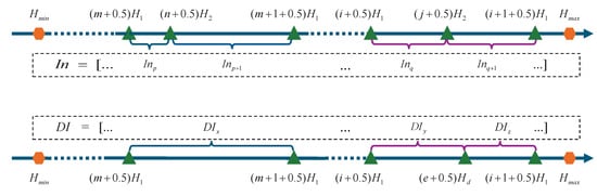
Figure 5. Cluster distribution of original phase group and differential phase group on the height line.

Set $d_{In}$ as the original intercept distance threshold and $d_{DI}$ as the differential intercept distance threshold. 

$$d_{In}=\mu \ast \underset{{In}_i\in In,{In}_j\in In,{In}_i\ne {In}_j}{min}|{In}_i-{In}_j|$$

(17)

$$d_{DI}=\mu \ast \underset{{DI}_m\in DI,{DI}_n\in DI,{DI}_m\ne {DI}_n}{min}|{DI}_m-{DI}_n|$$

(18)

Based on practical experience, the value of intercept distance threshold coefficient $\mu$ typically falls within the range of 0.3 to 0.5.

The $(a,b)$ pixel represents a pixel in an interferogram, with the horizontal coordinate represented by a and the vertical coordinate represented by b. The actual original intercept and actual differential intercept of the $(a,b)$ pixel are denoted by $\widetilde{In}(a,b)$ and $\widetilde{DI}(a,b)$, respectively. The actual original intercept distance of the $(a,b)$ pixel is given as follows:

$$DisIn(a,b)=\underset{{In}_i\in In}{min}|\widetilde{In}(a,b)-{In}_i|$$

(19)

The actual differential intercept distance of the $(a,b)$ pixel is given as follows:

$$DisDI(a,b)=\underset{{DI}_j\in DI}{min}|\widetilde{DI}(a,b)-{DI}_j|$$

(20)

The intercept filtering is illustrated below in four scenarios. The filtered original intercept and filtered differential intercept of the $(a,b)$ pixel are denoted by $\widehat{In}(a,b)$ and $\widehat{DI}(a,b)$, respectively.

Scenario 1: $d_{In}>DisIn(a,b)$ and $d_{DI}>DisDI(a,b)$.

Filter $\widetilde{In}(a,b)$ and $\widetilde{DI}(a,b)$ according to (21) and (22), then replace actual values with filtered results.

$$\widehat{In}(a,b)=\underset{{In}_i\in In}{argmin}\left|\widetilde{In}(a,b)-I{n}_i\right|$$

(21)

$$\widehat{DI}(a,b)=\underset{D{I}_j\in DI}{argmin}\left|\widetilde{DI}(a,b)-D{I}_j\right|$$

(22)

Scenario 2: $d_{In}<DisIn(a,b)$ and $d_{DI}>DisDI(a,b)$.

Since $d>DisDI(a,b)$, therefore $\widehat{DI}(a,b)$ can be obtained according to (22). Then, the $H_1$ height space which $\widehat{DI}(a,b)$ belongs to is determined. The $I{n}_{H_1}$ of the $H_1$ height space is founded and the intercept filtering process is performed according to (23). For example, the $(a,b)$ pixel satisfies $\widehat{DI}(a,b)$ = $D{I}_x$, which means that it is in the $((m+0.5)H_1$, $(m+1+0.5)H_1)$ height space, hence the $I{n}_{H_1}$ = [$I{n}_p$, $I{n}_{p+1}$] used in solving for $\widehat{In}(a,b)$ according to (23).

$$\widehat{In}(a,b)=\underset{I{n}_d\in I{n}_{H_1}}{argmin}\left|\widetilde{In}(a,b)-I{n}_d\right|$$

(23)

Scenario 3: $d_{In}>DisIn(a,b)$ and $d_{DI}<DisDI(a,b)$.

Since $d>DisIn(a,b)$, therefore $\widehat{In}(a,b)$ can be obtained according to (21). Then, a $H_1$ height space which $\widehat{In}(a,b)$ belonging to is determined. The $D{I}_{H_1}$ of the $H_1$ height space is founded and the intercept filtering process is performed according to (24). For example, the $(a,b)$ pixel satisfies $\widehat{In}(a,b)$ = $I{n}_q$, which means that it is in the $((i+0.5)H_1$, $(i+1+0.5)H_1)$ height space, hence the $D{I}_{H_1}$ = [$D{I}_y$, $D{I}_z$] used in solving for $\widehat{DI}(a,b)$ according to (24).

$$\widehat{DI}(a,b)=\underset{D{I}_e\in D{I}_{H_1}}{argmin}\left|\widetilde{DI}(a,b)-D{I}_e\right|$$

(24)

Scenario 4: $d_{In}<DisIn(a,b)$ and $d_{DI}<DisDI(a,b)$.

According to (21) and (22), $\widehat{In}(a,b)$ and $\widehat{DI}(a,b)$ can be obtained. If $\widehat{In}(a,b)$ and $\widehat{DI}(a,b)$ belong to the same $H_1$ height space, $\widehat{In}(a,b)$ and $\widehat{DI}(a,b)$ are considered reliable. If $\widehat{In}(a,b)$ and $\widehat{DI}(a,b)$ do not belong to the same $H_1$ height space, $\widehat{In}(a,b)$ and $\widehat{DI}(a,b)$ are considered unreliable. These pixels with unreliable intercepts are marked with flag bits, indicating that these pixels are too affected by noise to be processed efficiently.

The proposed intercept filtering method effectively addresses two critical challenges: (1) phase noise-induced errors in intercept determination, and (2) computational inefficiency in intercept search. This method guarantees intercept accuracy while eliminating the need for search procedures. After the intercept filtering process is complete, all pixels except those flagged as anomalous will have error-free intercept values that should lie within the theoretical intercept vector. The pixels are then grouped into clusters after the intercept filtering. The cluster groups are formed of pixels that have identical intercept values and have not been marked as anomalous. The filtered original intercepts and filtered differential intercepts of these cluster groups are denoted by […, ${\widehat{In}}_p$, ${\widehat{In}}_{p+1}$, …, ${\widehat{In}}_q$, ${\widehat{In}}_{q+1}$, …] and […, ${\widehat{DI}}_x$, …, ${\widehat{DI}}_y$, ${\widehat{DI}}_z$, …], respectively.

3.4. Closed-Form Ambiguity Number Solution

Filtered error-free intercept vectors can be obtained after the process described in the previous three subsections. In this subsection, the closed-form ambiguity number is derived by constructing and solving CRT equation groups whose error-free intercepts are used as remainders. It mitigates the effect of phase noise on ambiguity number determination and avoids ambiguity number search.

Each $H_1$ height space corresponds to one CRT equation group. Each CRT equation group consists of an original phase group CRT Equation (5) and a differential phase group CRT Equation (12). The number of the ambiguity number $k_1$ is N:

$$N=\lceil {\displaystyle \frac{H_{max}-0.5H_1}{H_1}}\rceil -\lceil {\displaystyle \frac{H_{min}-0.5H_1}{H_1}}\rceil +1$$

(25)

This means that there are N CRT equation groups to be solved.

An example is given below to illustrate the detailed solution process. The cluster distribution of the original phase group is shown at the top of Figure 6. The cluster distribution of the differential phase group is shown at the bottom of Figure 6. For the $H_1$ height space in Figure 6, the original phase group has two cluster groups, while the differential phase group has one cluster group. $k_1\left(m\right)$ corresponds to $k_2(n-1)$ and $k_2\left(n\right)$, which can form (26) and (27):

$$k_1\left(m\right)={\displaystyle \frac{B_1}{B_2}}{k}_2(n-1)+{\widehat{In}}_p$$

(26)

$$k_1\left(m\right)={\displaystyle \frac{B_1}{B_2}}{k}_2\left(n\right)+{\widehat{In}}_{p+1}$$

(27)

${\widehat{In}}_p$ and ${\widehat{In}}_{p+1}$ are the filtered original intercepts of the corresponding cluster groups. $k_1\left(m\right)$ corresponds to $k_d(x-1)$ which can form (28):

$$k_1\left(m\right)={\displaystyle \frac{B_1}{B_d}}{k}_d(x-1)+{\widehat{DI}}_x$$

(28)

${\widehat{DI}}_x$ is the filtered differential intercept of the corresponding cluster group.

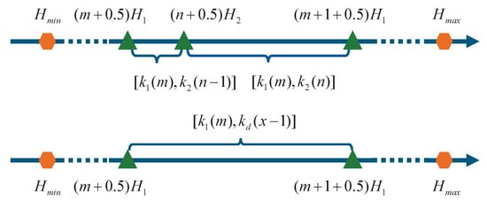
Figure 6. Explanation of the closed-form ambiguity number solution.

A CRT equation group is formed by selecting an equation from (26) or (27) and combining it with (28). (26) and (28) are used as an illustrative example in the following demonstration.

To satisfy the solvability conditions of the CRT equation group, a primary decomposition must be performed first:

$$\left\{\begin{array}{c}\hfill {\displaystyle \frac{B_1}{B_2}}=C\ast C_1\\ \hfill {\displaystyle \frac{B_1}{B_d}}=C\ast C_2\end{array}\right.$$

(29)

C is the common multiplicative factor, while $C_1$ and $C_2$ are a pair of coprime integers. Then define the following: 

$$\left\{\begin{array}{c}\hfill r_1=⌊{\displaystyle \frac{{\widehat{In}}_p}{C}}⌋\\ \hfill r_2=⌊{\displaystyle \frac{{\widehat{DI}}_x}{C}}⌋\end{array}\right.$$

(30)

where symbol $\lfloor ·\rfloor$ is the floor operation. Since remainders ${\widehat{In}}_p$ and ${\widehat{DI}}_x$ are filtered error-free intercepts, $r_1$ and $r_2$ in (30) are accurate. (26) and (28) are rewritten to yield the following equations:

$$\left\{\begin{array}{c}\hfill ⌊{\displaystyle \frac{k_1\left(m\right)}{C}}⌋=k_2(n-1)\ast C_1+r_1\\ \hfill ⌊{\displaystyle \frac{k_1\left(m\right)}{C}}⌋=k_d(x-1)\ast C_2+r_2\end{array}\right.$$

(31)

Consequently, the closed-form solution is as follows [21]:

$$⌊{\displaystyle \frac{k_1\left(m\right)}{C}}⌋=\sum _{i=1}^2\overline{{\gamma }_i}{\gamma }_i{r}_i\mathrm{mod}\mathsf{\Gamma }$$

(32)

$$\mathsf{\Gamma }=C_1\ast C_2$$

(33)

$${\gamma }_i={\displaystyle \frac{\mathsf{\Gamma }}{C_i}}$$

(34)

$\overline{{\gamma }_i}$ is the modular multiplicative inverse of ${\gamma }_i$ modulo $C_i$. Combining (26), (31) and (32) yields the following:

$$k_1\left(m\right)=C\ast \left(\sum _{i=1}^2\overline{{\gamma }_i}{\gamma }_i{r}_i\mathrm{mod}\mathsf{\Gamma }-⌊{\displaystyle \frac{{\widehat{In}}_p}{C}}⌋\right)+{\widehat{In}}_p$$

(35)

$$k_2(n-1)=\left(\sum _{i=1}^2\overline{{\gamma }_i}{\gamma }_i{r}_i\mathrm{mod}\mathsf{\Gamma }-⌊{\displaystyle \frac{{\widehat{In}}_p}{C}}⌋\right)/C_1$$

(36)

The ambiguity number vector [$k_1\left(m\right)$, $k_2(n-1)$] corresponds to the $p-th$ cluster group in the original phase group in Figure 5, thus establishing the equivalence [$k_{1p}$, $k_{2p}$] = [$k_1\left(m\right)$, $k_2(n-1)$]. According to the closed-form solution principle above, the ambiguity number vector [$k_1$, $k_2$] for each cluster group can be derived. For pixels marked as having both unreliable original and differential intercepts, we temporarily exclude them from the closed-form ambiguity number calculation. This avoids the propagation of intercept unreliability to the ambiguity number solution. Subsequently, the phase gaps corresponding to the marked pixels are filled via spatial interpolation on the unwrapped phase map.

3.5. Algorithm Flow Description

In this subsection, the processing flow of the algorithm proposed in this paper is represented by the following pseudocode (Algorithm 2).

Algorithm 2 Improved Closed-Form Multi-Baseline PU Algorithm

Input:  Parameters $\lambda$, R, $\theta$, $H_{min}$, $H_{max}$, $B_i$ and ${\phi }_i$ for i = 1, 2 Output:  Reconstructed unwrapped phase      1: Compute ${\phi }_d$ via (8)      2: Compute M via (15)      3: Compute the theoretical interferometric phase vectors ${\phi }_{1the}$, ${\phi }_{2the}$ and ${\phi }_{dthe}$ via (16)      4: Compute theoretical original intercept vector $In$ and theoretical differential intercept vector $DI$ via (6) and (13), respectively      5: Compute actual original intercept $\widetilde{In}$ and actual differential intercept $\widetilde{DI}$ for all pixels via (6) and (13), respectively      6: Compute $d_{In}$ and $d_{DI}$ via (17) and (18), respectively      7: for each $(a,b)$ pixel do      8:    Compute $DisIn(a,b)$ and $DisDI(a,b)$ via (19) and (20), respectively      9:    if $d_{In}>DisIn(a,b)$ and $d_{DI}>DisDI(a,b)$ then      10:      Filter $\widetilde{In}(a,b)$ and $\widetilde{DI}(a,b)$ via (21) and (22), respectively      11:    end if      12:    if $d_{In}<DisIn(a,b)$ and $d_{DI}>DisDI(a,b)$ then      13:      Filter $\widetilde{In}(a,b)$ and $\widetilde{DI}(a,b)$ via (23) and (22), respectively      14:    end if      15:    if $d_{In}>DisIn(a,b)$ and $d_{DI}<DisDI(a,b)$ then      16:      Filter $\widetilde{In}(a,b)$ and $\widetilde{DI}(a,b)$ via (21) and (24), respectively      17:    end if      18:    if $d_{In}<DisIn(a,b)$ and $d_{DI}<DisDI(a,b)$ then      19:      Filter $\widetilde{In}(a,b)$ and $\widetilde{DI}(a,b)$ via (21) and (22), respectively, or mark with flag bits      20:    end if      21: end for      22: Cluster pixels by the filtered original intercept $\widehat{In}$ and the filtered differential intercept $\widehat{DI}$ of all pixels, respectively      23: Compute N via (25)      24: for each cluster group do      25:    Compute $k_1$ and $k_2$ via (35) and (36), respectively      26: end for      27: Obtain the unwrapped phase of the marked pixels through spatial interpolation of the unwrapped phase map      28: return Output

3.6. Generalization to Multi-Baseline Mode

The main difference between dual-baseline and multi-baseline modes is the number of baselines, which increases from two to three or more. Expanding to multiple baselines introduces several differences from the dual-baseline mode. The following section details the similarities and differences when extending dual-baseline to multi-baseline modes. It specifically addresses differential phase processing, theoretical intercept calculation, intercept filtering, and closed-form ambiguity number solution.

Differential phase processing: In dual-baseline mode, differential phase processing is essential for constructing a new cluster Equation (12). In multi-baseline mode, however, it is optional. Nevertheless, when certain interferograms in multi-baseline mode are unusable due to excessive noise, differential phase processing can provide an alternative input. Therefore, differential phase processing should be retained for the multi-baseline mode.

Theoretical intercept calculation: The calculation method for the number of theoretical intercepts and the theoretical intercept vector in the multi-baseline mode is identical to that of the dual-baseline mode, both employing the approach detailed in Section 3.2.

Intercept filtering:

Next, the process of intercept filtering in triple-baseline mode will be explained by referring to Figure 7. The cluster distribution of the Baseline 1 and Baseline 2 group is shown at the top of Figure 7. The cluster distribution of the Baseline 1 and Baseline 3 group is shown at the middle of Figure 7. The cluster distribution of the differential phase group is shown at the bottom of Figure 7. As shown in Figure 7: $InB12$ = […, $InB{12}_p$, $InB{12}_{p+1}$, …, $InB{12}_q$, $InB{12}_{q+1}$, …] is the theoretical original intercept vector of Baseline 1 and Baseline 2 group, $InB13$ = […, $InB{13}_o$, $InB{13}_{o+1}$, …, $InB{13}_u$, $InB{13}_{u+1}$, …] is the theoretical original intercept vector of Baseline 1 and Baseline 3 group, and $DIMB$ = […, ${DIMB}_x$, …, ${DIMB}_y$, ${DIMB}_z$, …] is the theoretical differential intercept vector. The intersection of endpoints [$H_{min}$, …, $(m+0.5)H_1$, $(m+1+0.5)H_1$, …, $(i+0.5)H_1$, $(i+1+0.5)H_1$, …, $H_{max}$] with the height line can yield multiple non-overlapping line segments, which are defined as $H_1$ height spaces. The theoretical intercept vectors corresponding to the $H_1$ height space for the Baseline 1 and Baseline 2 group, the Baseline 1 and Baseline 3 group, and the differential phase group are $InB{12}_{H_1}$, $InB{13}_{H_1}$, and $DIM{B}_{H_1}$ respectively. For example, $((m+0.5)H_1$, $(m+1+0.5)H_1)$ in Figure 7 corresponds to $InB{12}_{H_1}$ = [$InB{12}_p$, $InB{12}_{p+1}$], $InB{13}_{H_1}$ = [$InB{13}_o$, $InB{13}_{o+1}$], $DIM{B}_{H_1}$ = [$DIM{B}_x$].

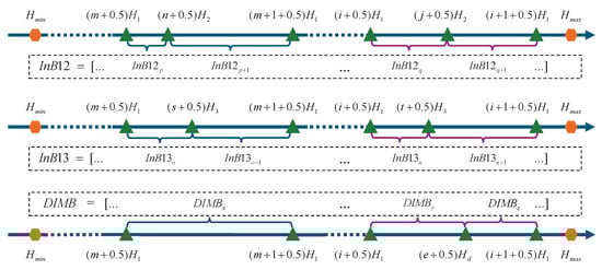
Figure 7. Cluster distribution of triple-baseline mode.

Set $d_{InB12}$ as Baseline 1 and Baseline 2 group distance threshold, $d_{InB13}$ as Baseline 1 and Baseline 3 group distance threshold, and $d_{DIMB}$ as the differential intercept distance threshold.

$$d_{InB12}=\mu \ast \underset{{InB12}_i\in InB12,{InB12}_j\in InB12,{InB12}_i\ne {InB12}_j}{min}|{InB12}_i-{InB12}_j|$$

(37)

$$d_{InB13}=\mu \ast \underset{{InB13}_i\in InB13,{InB13}_j\in InB13,{InB13}_i\ne {InB13}_j}{min}|{InB13}_i-{InB13}_j|$$

(38)

$$d_{DIMB}=\mu \ast \underset{{DIMB}_m\in DIMB,{DIMB}_n\in DIMB,{DIMB}_m\ne {DIMB}_n}{min}|{DIMB}_m-{DIMB}_n|$$

(39)

Based on practical experience, the value of $\mu$ typically falls within the range of 0.3 to 0.5.

$\widetilde{InB12}(a,b)$, $\widetilde{InB13}(a,b)$, $\widetilde{DIMB}(a,b)$ represent the actual intercept of the Baseline 1 and Baseline 2 group, the Baseline 1 and Baseline 3 group, and the differential phase group for the $(a,b)$ pixel, respectively. The actual intercept distance of the Baseline 1 and Baseline 2 groups of the $(a,b)$ pixel is given as follows:

$$DisInB12(a,b)=\underset{{InB12}_i\in InB12}{min}|\widetilde{InB12}(a,b)-{InB12}_i|$$

(40)

The actual intercept distance of the Baseline 1 and Baseline 3 groups of the $(a,b)$ pixel is given as follows:

$$DisInB13(a,b)=\underset{{InB13}_i\in InB13}{min}|\widetilde{InB13}(a,b)-{InB13}_i|$$

(41)

The actual differential intercept distance of the $(a,b)$ pixel is given as follows:

$$DisDIMB(a,b)=\underset{{DIMB}_j\in DIMB}{min}|\widetilde{DIMB}(a,b)-{DIMB}_j|$$

(42)

The intercept filtering is illustrated below in three scenarios. $\widehat{InB12}(a,b)$, $\widehat{InB13}(a,b)$, $\widehat{DIMB}(a,b)$ represent the filtered intercept of the Baseline 1 and Baseline 2 group, the Baseline 1 and Baseline 3 group, and the differential phase group for the $(a,b)$ pixel, respectively.

Scenario 1: All of $d_{InB12}>DisInB12(a,b)$, $d_{InB13}>DisInB13(a,b)$ and $d_{DIMB}>DisDIMB(a,b)$ are satisfied.

Filter $\widetilde{InB12}(a,b)$, $\widetilde{InB13}(a,b)$, $\widetilde{DIMB}(a,b)$ according to (43), (44), and (45), respectively. Then replace actual values with filtered results.

$$\widehat{InB12}(a,b)=\underset{{InB12}_i\in InB12}{argmin}\left|\widetilde{InB12}(a,b)-I{nB12}_i\right|$$

(43)

$$\widehat{InB13}(a,b)=\underset{{InB13}_i\in InB13}{argmin}\left|\widetilde{InB13}(a,b)-I{nB13}_i\right|$$

(44)

$$\widehat{DIMB}(a,b)=\underset{D{IMB}_j\in DIMB}{argmin}\left|\widetilde{DIMB}(a,b)-D{IMB}_j\right|$$

(45)

Scenario 2: At least one of $d_{InB12}>DisInB12(a,b)$, $d_{InB13}>DisInB13(a,b)$ or $d_{DIMB}>DisDIMB(a,b)$ is satisfied, but not all of them are satisfied. Below is a detailed explanation with an example where $d_{DIMB}>DisDIMB(a,b)$ is satisfied, but conditions $d_{InB12}>DisInB12(a,b)$ and $d_{InB13}>DisInB13(a,b)$ are not.

Since $d_{DIMB}>DisDIMB(a,b)$, therefore $\widehat{DIMB}(a,b)$ can be obtained according to (45). Then, a $H_1$ height space which $\widehat{DIMB}(a,b)$ belonging to is determined. The $InB{12}_{H_1}$ and The $InB{13}_{H_1}$ of the $H_1$ height space are founded and the intercept filtering process is performed according to (46) and (47). For example, the $(a,b)$ pixel satisfies $\widehat{DIMB}(a,b)$ = $DIM{B}_x$, which means that it is in the $((m+0.5)H_1$, $(m+1+0.5)H_1)$ height space, hence $InB{12}_{H_1}$ = [$InB{12}_p$, $InB{12}_{p+1}$] and $InB{13}_{H_1}$ = [$InB{13}_o$, $InB{13}_{o+1}$] used in solving for $\widehat{InB12}(a,b)$ and $\widehat{InB13}(a,b)$ according to (46) and (47), respectively.

$$\widehat{InB12}(a,b)=\underset{InB{12}_i\in InB{12}_{H_1}}{argmin}\left|\widetilde{InB12}(a,b)-InB{12}_i\right|,$$

(46)

$$\widehat{InB13}(a,b)=\underset{InB{13}_i\in InB{13}_{H_1}}{argmin}\left|\widetilde{InB13}(a,b)-InB{13}_i\right|,$$

(47)

Scenario 3: Neither $d_{InB12}>DisInB12(a,b)$, $d_{InB13}>DisInB13(a,b)$, nor $d_{DIMB}>DisDIMB(a,b)$ is satisfied.

According to (43)–(45), $\widehat{InB12}(a,b)$, $\widehat{InB13}(a,b)$ and $\widehat{DIMB}(a,b)$ can be obtained. If $\widehat{InB12}(a,b)$, $\widehat{InB13}(a,b)$ and $\widehat{DIMB}(a,b)$ belong to the same $H_1$ height space, $\widehat{InB12}(a,b)$, $\widehat{InB13}(a,b)$ and $\widehat{DIMB}(a,b)$ are considered reliable. If $\widehat{InB12}(a,b)$, $\widehat{InB13}(a,b)$ and $\widehat{DIMB}(a,b)$ do not belong to the same $H_1$ height space, $\widehat{InB12}(a,b)$, $\widehat{InB13}(a,b)$ and $\widehat{DIMB}(a,b)$ are considered unreliable. These pixels with unreliable intercepts are marked with flag bits, indicating that these pixels are too affected by noise to be processed efficiently.

The pixels are then grouped into clusters after the intercept filtering. The cluster groups are formed of pixels that have identical intercept values and have not been marked as anomalous. The filtered intercepts of the Baseline 1 and Baseline 2 group, the Baseline 1 and Baseline 3 group, and the differential phase group of these cluster groups are denoted by […, ${\widehat{InB12}}_p$, ${\widehat{InB12}}_{p+1}$, …, ${\widehat{InB12}}_q$, ${\widehat{InB12}}_{q+1}$, …], […, ${\widehat{InB13}}_o$, ${\widehat{InB13}}_{o+1}$, …, ${\widehat{InB13}}_u$, ${\widehat{InB13}}_{u+1}$, …], and […, ${\widehat{DIMB}}_x$, …, ${\widehat{DIMB}}_y$, ${\widehat{DIMB}}_z$, …], respectively. If the number of baselines exceeds three, intercept filtering could be implemented by making appropriate modifications to the triple-baseline mode.

Closed-form ambiguity number solution:

Each $H_1$ height space corresponds to one CRT equation group. The number of ambiguity number $k_1$ is N by (25).

An example is given below to illustrate the detailed solution process for triple-baseline mode by combining Figure 7 and Figure 8. The cluster distribution of the Baseline 1 and Baseline 2 group is shown at the top of Figure 8. The cluster distribution of the Baseline 1 and Baseline 3 group is shown at the middle of Figure 8. The cluster distribution of the differential phase group is shown at the bottom of Figure 8. For the $H_1$ height space illustrated in Figure 8, the Baseline 1 and Baseline 2 group has two cluster groups, and the Baseline 1 and Baseline 3 group also has two cluster groups, while the differential phase group has only a single cluster group. In the Baseline 1 and Baseline 2 groups, $k_1\left(m\right)$ corresponds to $k_2(n-1)$ and $k_2\left(n\right)$, which can form (48) and (49):

$$k_1\left(m\right)={\displaystyle \frac{B_1}{B_2}}{k}_2(n-1)+{\widehat{InB12}}_p$$

(48)

$$k_1\left(m\right)={\displaystyle \frac{B_1}{B_2}}{k}_2\left(n\right)+{\widehat{InB12}}_{p+1}$$

(49)

${\widehat{InB12}}_p$ and ${\widehat{InB12}}_{p+1}$ are the filtered original intercepts of the corresponding cluster groups in the Baseline 1 and Baseline 2 groups.

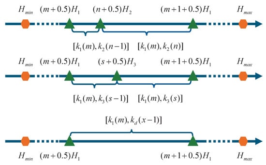
Figure 8. Explanation of the closed-form ambiguity number solution for triple-baseline mode.

In the Baseline 1 and Baseline 3 group, $k_1\left(m\right)$ corresponds to $k_3(s-1)$ and $k_3\left(s\right)$, which can form (50) and (51):

$$k_1\left(m\right)={\displaystyle \frac{B_1}{B_3}}{k}_3(s-1)+{\widehat{InB13}}_o$$

(50)

$$k_1\left(m\right)={\displaystyle \frac{B_1}{B_3}}{k}_3\left(s\right)+{\widehat{InB13}}_{o+1}$$

(51)

${\widehat{InB13}}_o$ and ${\widehat{InB13}}_{o+1}$ are the filtered original intercepts of the corresponding cluster groups in the Baseline 1 and Baseline 3 groups.

In the differential phase group, $k_1\left(m\right)$ corresponds to $k_d(x-1)$ which can form (52):

$$k_1\left(m\right)={\displaystyle \frac{B_1}{B_d}}{k}_d(x-1)+{\widehat{DIMB}}_x$$

(52)

${\widehat{DIMB}}_x$ is the filtered intercept of the corresponding cluster group in the differential phase group.

(48), (50) and (52) are used as an illustrative example in the following demonstration.

To satisfy the solvability conditions of the CRT equation group, a primary decomposition must be performed first:

$$\left\{\begin{array}{c}\hfill {\displaystyle \frac{B_1}{B_2}}=C\ast C_1\\ \hfill {\displaystyle \frac{B_1}{B_3}}=C\ast C_2\\ \hfill {\displaystyle \frac{B_1}{B_d}}=C\ast C_3\end{array}\right.$$

(53)

C is the common multiplicative factor, while $C_1$, $C_2$, and $C_3$ are coprime integers. Then define:

$$\left\{\begin{array}{c}\hfill r_1=⌊{\displaystyle \frac{{\widehat{InB12}}_p}{C}}⌋\\ \hfill r_2=⌊{\displaystyle \frac{{\widehat{InB13}}_o}{C}}⌋\\ \hfill r_3=⌊{\displaystyle \frac{{\widehat{DIMB}}_x}{C}}⌋\end{array}\right.$$

(54)

Since remainders ${\widehat{InB12}}_p$, ${\widehat{InB13}}_o$ and ${\widehat{DIMB}}_x$ are filtered error-free intercepts, $r_1$, $r_2$ and $r_3$ in (54) are accurate. (48), (50) and (52) are rewritten to yield the following equations:

$$\left\{\begin{array}{c}\hfill ⌊{\displaystyle \frac{k_1\left(m\right)}{C}}⌋=k_2(n-1)\ast C_1+r_1\\ \hfill ⌊{\displaystyle \frac{k_1\left(m\right)}{C}}⌋=k_3(s-1)\ast C_2+r_2\\ \hfill ⌊{\displaystyle \frac{k_1\left(m\right)}{C}}⌋=k_d(x-1)\ast C_3+r_3\end{array}\right.$$

(55)

Consequently, the closed-form solution is [21]:

$$⌊{\displaystyle \frac{k_1\left(m\right)}{C}}⌋=\sum _{i=1}^3\overline{{\gamma }_i}{\gamma }_i{r}_i\mathrm{mod}\mathsf{\Gamma }$$

(56)

$$\mathsf{\Gamma }=C_1\ast C_2\ast C_3$$

(57)

$${\gamma }_i={\displaystyle \frac{\mathsf{\Gamma }}{C_i}}$$

(58)

$\overline{{\gamma }_i}$ is modular multiplicative inverse of ${\gamma }_i$ modulo $C_i$. Therefore, the following results can be obtained:

$$k_1\left(m\right)=C\ast \left(\sum _{i=1}^3\overline{{\gamma }_i}{\gamma }_i{r}_i\mathrm{mod}\mathsf{\Gamma }-⌊{\displaystyle \frac{{\widehat{InB12}}_p}{C}}⌋\right)+{\widehat{InB12}}_p$$

(59)

$$k_2(n-1)=\left(\sum _{i=1}^3\overline{{\gamma }_i}{\gamma }_i{r}_i\mathrm{mod}\mathsf{\Gamma }-⌊{\displaystyle \frac{{\widehat{InB12}}_p}{C}}⌋\right)/C_1$$

(60)

$$k_3(s-1)=\left(\sum _{i=1}^3\overline{{\gamma }_i}{\gamma }_i{r}_i\mathrm{mod}\mathsf{\Gamma }-⌊{\displaystyle \frac{{\widehat{InB13}}_o}{C}}⌋\right)/C_2$$

(61)

According to the closed-form solution principle above, the ambiguity number vector [$k_1$, $k_2$] or [$k_1$, $k_3$] for each cluster group can be derived. If the number of baselines exceeds three, a closed-form ambiguity number solution could be implemented by making appropriate modifications to the triple-baseline mode.

4. Performance Analysis

In order to validate the effectiveness of the improved closed-form multi-baseline PU algorithm proposed in this article, experiments are conducted on a simulated dataset and two real datasets. All three experiments compare the proposed algorithm with the PU-max-flow algorithm (PUMA) [38], the conventional CA algorithm [30], the MBPUF algorithm [33], and the cluster correction algorithms [35] in terms of accuracy and efficiency. In all experiments, accuracy is represented by the PU success rate (PUSR) [35], the root mean square error (RMSE), and the unwrapping residual maps. The window size in the cluster correction algorithm is uniformly set to 9 × 9. The computer used in three experiments has an Intel(R) Core(TM) i9-10885H processor running @ 2.4 GHz, with 64 GB of memory.

The first experiment is carried out using simulated data, which comprised 1140 × 1174 pixels. The reference DEM for the simulated scenario is shown in Figure 9a. The geometric configuration is a one-transmitter and three-receiver mode, where satellite 1 transmits signals while satellites 1, 2, and 3 receive simultaneously, forming two vertical effective baselines. The detailed parameters are given in Table 1.

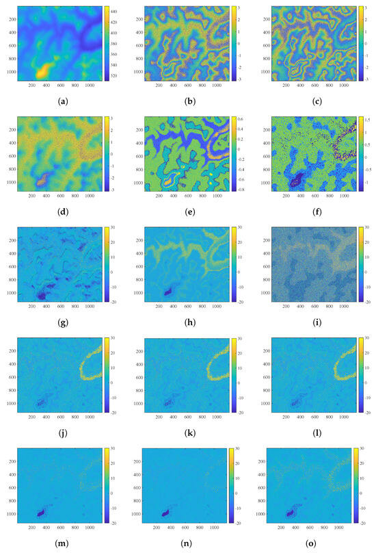
Figure 9. (a) Reference DEM (unit: m). (b) Noisy interferometric phase of $B_1$ (unit: rad). (c) Noisy interferometric phase of $B_2$ (unit: rad). (d) Differential interferometric phase (unit: rad). (e) Filtered intercepts of the original phase group. (f) Filtered intercepts of the differential phase group. (g) Reconstructed phase error by the PUMA algorithm (unit: rad). (h) Reconstructed phase error by the conventional CA algorithm (unit: rad). (i) Reconstructed phase error by the MBPUF algorithm (unit: rad). (j) Reconstructed phase error by the PPCC algorithm (unit: rad). (k) Reconstructed phase error by the NPCC1 algorithm (unit: rad). (l) Reconstructed phase error by the NPCC2 algorithm (unit: rad). (m) Reconstructed phase error by the proposed algorithm under the condition of 1 rad noise (unit: rad). (n) Reconstructed phase error by the proposed algorithm under the condition of 0.8 rad noise (unit: rad). (o) Reconstructed phase error by the proposed algorithm under the condition of 1.2 rad noise (unit: rad).

Table 1. Parameters of simulated data.

Frequency	X-band
Orbital Altitude	500 km
Incidence Angle	40°
Length of $B_1$	297.6 m
Length of $B_2$	401.1 m
Ambiguity Height of $B_1$	43.5 m
Ambiguity Height of $B_2$	32.3 m

Figure 9b shows the noisy interferometric phase of $B_1$, and Figure 9c shows the noisy interferometric phase of $B_2$. Both Figure 9b,c are subjected to Gaussian white noise with a standard deviation of 1 rad. Figure 9d–m are the results under this noise condition Figure 9d shows the differential interferometric phase formed by combining Figure 9b,c. Figure 9e shows the filtered intercepts of the original phase group. Figure 9f shows the filtered intercepts of the differential phase group.

The following describes the unwrapping of residual maps, represented here by reconstructed phase errors. Figure 9g shows reconstructed phase error by the PUMA algorithm. Figure 9h shows the reconstructed phase error by the conventional CA algorithm. Figure 9i shows the reconstructed phase error by the MBPUF algorithm. Figure 9j shows the reconstructed phase error by the pixel-by-pixel cluster correction (PPCC) algorithm. Figure 9k shows the reconstructed phase error by the first non-core pixel cluster correction (NPCC1) algorithm. Figure 9l shows the reconstructed phase error by the second noncore pixel cluster correction (NPCC2) algorithm. Figure 9m shows the reconstructed phase error by the proposed algorithm.

At the same time, in order to verify the performance of the proposed algorithm under different noise conditions, we also set Gaussian white noise of 0.8 rad and 1.2 rad, respectively. Figure 9n shows the reconstructed phase error by the proposed algorithm under the condition of 0.8 rad noise. Figure 9o shows the reconstructed phase error by the proposed algorithm under the condition of 1.2 rad noise.

The accuracy results of these algorithms for the simulated data are shown in Table 2. As can be seen from Table 2 and Figure 9, the PUMA algorithm and the conventional CA algorithm produce significant phase errors due to phase noise. The three distinct cluster correction algorithms (PPCC, NPCC1, and NPCC2) correct the original cluster numbers to different degrees, thereby enhancing the accuracy of the conventional CA algorithm. Furthermore, the proposed algorithm demonstrates superior performance compared to the other algorithms, as shown by results for PUSR, RMSE and the reconstructed phase error results in Figure 9. Additionally, it can be seen that there are many errors in the results of the MBPUF algorithm. The MBPUF algorithm provides a set of all possible theoretical intercepts, from which the one corresponding to the actual intercept is selected based on the nearest principle. In this algorithm, all possible theoretical intercepts are determined by the coprime numbers ${\mathsf{\Gamma }}_1$ and ${\mathsf{\Gamma }}_2$ of ambiguity height $H_1$ and $H_2$. The range is (−1, ${\mathsf{\Gamma }}_1$/${\mathsf{\Gamma }}_2$) and the quantity is ${\mathsf{\Gamma }}_1$ + ${\mathsf{\Gamma }}_2$− 1. When ${\mathsf{\Gamma }}_1$ and ${\mathsf{\Gamma }}_2$ are particularly large, all possible theoretical intercept distributions become very dense. Therefore, when phase errors exist, and all possible theoretical intercept distributions are particularly dense, the theoretical intercepts found by the nearest principle are most susceptible to errors. In this dataset, ${\mathsf{\Gamma }}_1$ is 435 and ${\mathsf{\Gamma }}_2$ is 323. The MBPUF algorithm requires the theoretical intercept to be found from among 757 possible theoretical intercepts within the range (−1, 435/323), which results in a relatively large number of reconstructed phase errors. In addition, the accuracy of the proposed algorithm remains at a relatively stable level at all times under the influence of phase noise at 0.8 rad, 1 rad, and 1.2 rad.

Table 2. Accuracy and efficiency statistics for the simulated data.

	Added Noise (Unit: rad)	PUSR	RMSE (Unit: rad)	Time (Unit: s)
PUMA	1	78.43%	7.62	89.33
conventional CA	1	81.64%	6.36	13.25
MBPUF	1	47.13%	18.93	44.19
PPCC	1	90.04%	3.31	18.79
NPCC1	1	89.75%	3.42	17.26
NPCC2	1	89.39%	3.47	16.83
proposed algorithm	1	93.87%	2.66	4.85
proposed algorithm	0.8	94.85%	2.35	4.73
proposed algorithm	1.2	92.22%	2.97	4.88

The processing time of these algorithms for simulated data are shown in Table 2. The times in the table only include the processing time of each algorithm and do not include the time spent reading the dataset and auxiliary files. The PUMA algorithm takes 89.33 s. The conventional CA algorithm requires searching for the cluster centerlines. It also requires searching for the ambiguity number. This takes 13.25 s. The three cluster correction algorithms (PPCC, NPCC1, and NPCC2) require adjustments to the conventional CA algorithm, yielding computational times of 18.79, 17.26, and 16.83 s, respectively. The MBPUF algorithm needs to search for the nearest theoretical intercept among 757 theoretical intercepts, which takes 44.19 s. The proposed algorithm requires only intercept filtering based on 8 theoretical intercepts, eliminating the need for an intercept search. Meanwhile, it adopts a closed-form solution to avoid the ambiguous-number search, resulting in a computation time of 4.85 s. In addition, it can be observed that different levels of noise have little impact on the time consumption of the proposed algorithm.

The second experiment demonstrates the effectiveness of the proposed algorithm on TanDEM-X datasets. The observation area is located on Java Island, Indonesia, with central coordinates at [110.87°E, 7.38°S]. Figure 10a shows the reference DEM of the observation area, and specific parameters are listed in Table 3.

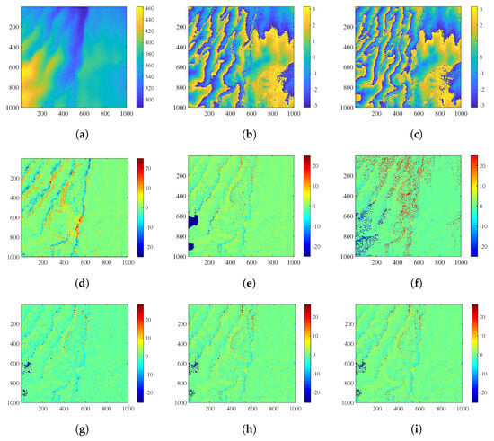
Figure 10. (a) Reference DEM (unit: m). (b) Noisy interferometric phase of $B_1$ (unit: rad). (c) Noisy interferometric phase of $B_2$ (unit: rad). (d) Reconstructed phase error by the PUMA algorithm (unit: rad). (e) Reconstructed phase error by the conventional CA algorithm (unit: rad). (f) Reconstructed phase error by the MBPUF algorithm (unit: rad). (g) Reconstructed phase error by the PPCC algorithm (unit: rad). (h) Reconstructed phase error by the NPCC1 algorithm (unit: rad). (i) Reconstructed phase error by the NPCC2 algorithm (unit: rad).

Table 3. Parameters of TanDEM-X Data.

Interferogram	1	2
Observation Time	2013-01-17	2012-12-15
Incidence Angle	32.18°	32.16°
Vertical Baseline	82.9 m	107.5 m
Ambiguity Height	55.3 m	42.7 m

Figure 10b shows the noisy interferometric phase of $B_1$, and Figure 10c shows the noisy interferometric phase of $B_2$. The reference phase used for comparison is generated based on the high-precision TanDEM-X DEM. Figure 10d shows reconstructed phase error by the PUMA algorithm. Figure 10e shows reconstructed phase error by the conventional CA algorithm, where clear phase jumps can be seen in the left region. Figure 10f shows the reconstructed phase error by the MBPUF algorithm. Figure 10g shows the reconstructed phase error by the PPCC algorithm. Figure 10h shows the reconstructed phase error by the NPCC1 algorithm. Figure 10i shows the reconstructed phase error by the NPCC2 algorithm. Figure 11a shows differential interferometric phase. Figure 11b shows filtered original intercepts obtained by filtering intercepts formed from Figure 10b,c and Figure 11c shows filtered differential intercepts obtained by filtering intercepts formed from Figure 10b and Figure 11a. Figure 11d shows reconstructed phase error by the proposed algorithm combining Figure 11b and Figure 11c.

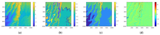
Figure 11. (a) Differential interferometric phase (unit: rad). (b) Filtered original intercepts obtained by filtering intercepts formed from Figure 10b,c. (c) Filtered differential intercepts obtained by filtering intercepts formed from Figure 10b and (a). (d) Reconstructed phase error by the proposed algorithm combining (b,c) (unit: rad).

The reconstructed phase error results of these algorithms for the TanDEM-X data are shown in Table 4. As demonstrated by Table 4 and Figure 10, the PUMA algorithm, the conventional CA algorithm, and the MBPUF algorithm exhibit significant phase errors. The three cluster correction algorithms (PPCC, NPCC1, and NPCC2) effectively mitigate the errors inherent in the conventional CA algorithm. The proposed algorithm achieves the highest accuracy, with PUSR and RMSE values of 94.47% and 2.38 rad, respectively. The processing time of these algorithms for the TanDEM-X data are shown in Table 4. The processing times are as follows: 68.19 s for the PUMA algorithm, 6.79 s for the conventional CA algorithm, 8.28 s for the MBPUF algorithm, 11.21 s for the PPCC algorithm, 9.38 s for the NPCC1 algorithm, 9.47 s for the NPCC2 algorithm, and 4.77 s for the proposed algorithm.

Table 4. Accuracy and efficiency statistics for the TanDEM-X data.

	PUSR	RMSE (Unit: rad)	Time (Unit: s)
PUMA	88.67%	6.13	68.19
conventional CA	91.35%	4.18	6.79
MBPUF	86.33%	7.36	8.28
PPCC	93.11%	2.69	11.21
NPCC1	92.34%	2.93	9.38
NPCC2	92.17%	3.01	9.47
proposed algorithm	94.47%	2.38	4.77

The third experiment demonstrates the effectiveness of the proposed algorithm on data from the TH-2 satellite. Successfully launched on 30 April 2019, TH-2 operates in the X-band with a resolution of 3 m and a swath width of 30 km. It employs a bistatic formation with satellites in different orbital planes and an interferometric configuration of one transmitter and two receivers operating in stripmap mode [39]. The observation area is located in the Brazilian Highlands, with central coordinates at [37.08°W, 8.68°S]. The reference DEM is shown in Figure 12a, and specific parameters are listed in Table 5.

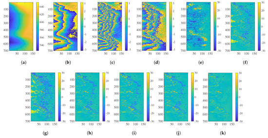
Figure 12. (a) Reference DEM (unit: m). (b) Noisy interferometric phase of $B_1$ (unit: rad). (c) Noisy interferometric phase of $B_2$ (unit: rad). (d) differential interferometric phase (unit: rad). (e) Reconstructed phase error by the PUMA algorithm (unit: rad). (f) Reconstructed phase error by the conventional CA algorithm (unit: rad). (g) Reconstructed phase error by the MBPUF algorithm (unit: rad). (h) Reconstructed phase error by the PPCC algorithm (unit: rad). (i) Reconstructed phase error by the NPCC1 algorithm (unit: rad). (j) Reconstructed phase error by the NPCC2 algorithm (unit: rad). (k) Reconstructed phase error by the proposed algorithm (unit: rad).

Table 5. Parameters of TH-2 data.

Interferogram	1	2
Observation Time	2021-08-21	2021-11-22
Incidence Angle	38.87°	38.95°
Vertical Baseline	130.9 m	308.1 m
Ambiguity Height	51.3 m	21.8 m

Figure 12b shows the noisy interferometric phase of $B_1$, and Figure 12c shows the noisy interferometric phase of $B_2$. Figure 12d shows differential interferometric phase. The reference phase used for comparison is generated based on a high-precision TH-2 DEM. Figure 12e shows the reconstructed phase error by the PUMA algorithm. Figure 12f shows the reconstructed phase error by the conventional CA algorithm. Figure 12g shows the reconstructed phase error by the MBPUF algorithm. Figure 12h shows the reconstructed phase error by the PPCC algorithm. Figure 12i shows the reconstructed phase error by the NPCC1 algorithm. Figure 12j shows the reconstructed phase error by the NPCC2 algorithm. Figure 12k shows the reconstructed phase error by the proposed algorithm.

The reconstructed phase error results of these algorithms for the TH-2 data are shown in Table 6. As demonstrated by Table 6 and Figure 12, the PUMA algorithm, the conventional CA algorithm and the MBPUF algorithm exhibit significant phase errors. The three cluster correction algorithms (PPCC, NPCC1, and NPCC2) effectively mitigate the errors inherent in conventional CA; however, they still introduce obvious errors due to the loss of cluster groups. The proposed algorithm achieves the highest accuracy, with PUSR and RMSE values of 92.11% and 3.19 rad, respectively. Additionally, Table 6 provides the processing time for each algorithm when handling the TH-2 data. The specific processing times are as follows: the PUMA algorithm uses 37.39 s, the conventional CA algorithm takes 4.92 s, the MBPUF algorithm requires 13.08 s, the PPCC algorithm consumes 5.31 s, the NPCC1 algorithm takes 5.20 s, the NPCC2 algorithm uses 5.16 s, and the proposed algorithm achieves the shortest processing time of 2.64 s.

Table 6. Accuracy and efficiency statistics for the TH-2 data.

	PUSR	RMSE (Unit: rad)	Time (Unit: s)
PUMA	78.36%	6.85	37.39
conventional CA	83.17%	5.89	4.92
MBPUF	81.01%	6.32	13.08
PPCC	87.49%	4.28	5.31
NPCC1	87.06%	4.37	5.20
NPCC2	86.94%	4.42	5.16
proposed algorithm	92.11%	3.19	2.64

Experiments on simulated, TanDEM-X, and TH-2 data demonstrate that the proposed algorithm exhibits consistent performance characteristics across diverse scenarios, thoroughly validating its accuracy and efficiency. The algorithm strikes an effective balance between high phase-unwrapping precision and rapid computational speed.

5. Conclusions

This article proposes an improved closed-form multi-baseline PU algorithm to overcome the limitations of conventional CA algorithms, which are susceptible to phase noise and have low computational efficiency. This algorithm is also designed to satisfy the accuracy and efficiency requirements at the practical application level. The core innovations lie in four key advancements that distinguish it from conventional CAs. First, differential phase processing is introduced to extend the ambiguity height range, providing new inputs for subsequent ambiguity number solving. Second, a novel method of calculating theoretical intercepts has been developed. This method integrates external reference DEM data and ambiguity-height information to generate precise finite intercepts. This lays the foundation for efficient intercept filtering. Third, an intercept filtering strategy is proposed to mitigate the effects of phase noise. By filtering the actual intercepts of all pixels, this method eliminates the need for time-consuming intercept searches while ensuring accuracy. Fourth, a closed-form ambiguity number solution is obtained by constructing and solving CRT equations using filtered, error-free intercepts as remainders, thereby avoiding ambiguity number searches and reducing the impact of noise. To comprehensively validate the effectiveness of the proposed algorithm, three experiments are conducted. The experimental results show that the proposed algorithm improves both accuracy and processing efficiency. Our future work will explore combining this algorithm with pre-processing of phase and intercept to enhance its adaptability to extreme scenarios and large datasets.

References

- Bamler, R.; Hartl, P. Synthetic Aperture Radar Interferometry. Inverse Probl. 1998, 14, R1–R54. [Google Scholar] [CrossRef]
- Rosen, P.A.; Hensley, S.; Joughin, I.R.; Li, F.K.; Madsen, S.N.; Rodriguez, E.; Goldstein, R.M. Synthetic Aperture Radar Interferometry. Proc. IEEE 2000, 88, 333–382. [Google Scholar] [CrossRef]
- Toutin, T.; Gray, L. State-of-the-Art of Elevation Extraction from Satellite SAR Data. ISPRS J. Photogramm. Remote Sens. 2000, 55, 13–33. [Google Scholar] [CrossRef]
- Béjar-Pizarro, M.; Álvarez Gómez, J.A.; Staller, A.; Luna, M.P.; Pérez-López, R.; Monserrat, O.; Chunga, K.; Lima, A.; Galve, J.P.; Martínez Díaz, J.J.; et al. InSAR-Based Mapping to Support Decision-Making after an Earthquake. Remote Sens. 2018, 10, 899. [Google Scholar] [CrossRef]
- Devanthéry, N.; Crosetto, M.; Monserrat, O.; Cuevas-González, M.; Crippa, B. An Approach to Persistent Scatterer Interferometry. Remote Sens. 2014, 6, 6662–6679. [Google Scholar] [CrossRef]
- Tomás, R.; Pagán, J.I.; Navarro, J.A.; Cano, M.; Pastor, J.L.; Riquelme, A.; Cuevas-González, M.; Crosetto, M.; Barra, A.; Monserrat, O.; et al. Semi-Automatic Identification and Pre-Screening of Geological–Geotechnical Deformational Processes Using Persistent Scatterer Interferometry Datasets. Remote Sens. 2019, 11, 1675. [Google Scholar] [CrossRef]
- Zhao, J.; Wu, J.; Ding, X.; Wang, M. Elevation Extraction and Deformation Monitoring by Multitemporal InSAR of Lupu Bridge in Shanghai. Remote Sens. 2017, 9, 897. [Google Scholar] [CrossRef]
- Fornaro, G.; Pauciullo, A.; Sansosti, E. Phase Difference-Based Multichannel Phase Unwrapping. IEEE Trans. Image Process. 2005, 14, 960–972. [Google Scholar] [CrossRef]
- Yu, H.; Lan, Y.; Yuan, Z.; Xu, J.; Lee, H. Phase Unwrapping in InSAR: A Review. IEEE Geosci. Remote Sens. Mag. 2019, 7, 40–58. [Google Scholar] [CrossRef]
- Yu, H.; Li, Z.; Bao, Z. Residues Cluster-Based Segmentation and Outlier-Detection Method for Large-Scale Phase Unwrapping. IEEE Trans. Image Process. 2011, 20, 2865–2875. [Google Scholar] [CrossRef]
- Chen, C.; Zebker, H. Phase Unwrapping for Large SAR Interferograms: Statistical Segmentation and Generalized Network Models. IEEE Trans. Geosci. Remote Sens. 2002, 40, 1709–1719. [Google Scholar] [CrossRef]
- Lan, Y.; Yu, H.; Xing, M.; Plaza, A. A Cluster-Analysis and Convex Hull-Based Fast Large-Scale Phase Unwrapping Method for Single- and Multibaseline SAR Interferograms. IEEE J. Sel. Top. Appl. Earth Obs. Remote Sens. 2023, 16, 5416–5429. [Google Scholar] [CrossRef]
- Xu, W.; Chang, E.C.; Kwoh, L.K.; Lim, H.; Cheng, W.; Heng, A. Phase-Unwrapping of SAR Interferogram with Multi-Frequency or Multi-Baseline. In Proceedings of the IGARSS ’94—1994 IEEE International Geoscience and Remote Sensing Symposium, Pasadena, CA, USA, 8–12 August 1994; Volume 2, pp. 730–732. [Google Scholar] [CrossRef]
- Lombardini, F. Absolute Phase Retrieval in a Three-Element Synthetic Aperture Radar Interferometer. In Proceedings of the International Radar Conference, Beijing, China, 8–10 October 1996; pp. 309–312. [Google Scholar] [CrossRef]
- Pascazio, V.; Schirinzi, G. Estimation of Terrain Elevation by Multifrequency Interferometric Wide Band SAR Data. IEEE Signal Process. Lett. 2001, 8, 7–9. [Google Scholar] [CrossRef] [PubMed]
- Ferraiuolo, G.; Pascazio, V. A Bayesian Approach Based on Modified Markov Random Fields for Microwave Tomography. In Proceedings of the IEEE International Geoscience and Remote Sensing Symposium, Toronto, ON, Canada, 24–28 June 2002; Volume 6, pp. 3393–3395. [Google Scholar] [CrossRef]
- Ferraiuolo, G.; Pascazio, V.; Schirinzi, G. Maximum a Posteriori Estimation of Height Profiles in InSAR Imaging. IEEE Geosci. Remote Sens. Lett. 2004, 1, 66–70. [Google Scholar] [CrossRef]
- Li, Z.; Bao, Z.; Li, H.; Liao, G. Image Autocoregistration and InSAR Interferogram Estimation Using Joint Subspace Projection. IEEE Trans. Geosci. Remote Sens. 2006, 44, 288–297. [Google Scholar] [CrossRef]
- Guo, J.; Li, Z.; Bao, Z. Using Multibaseline InSAR to Recover Layovered Terrain Considering Wideband Array Problem. IEEE Geosci. Remote Sens. Lett. 2008, 5, 583–587. [Google Scholar] [CrossRef]
- Xia, X.; Wang, G. Phase Unwrapping and A Robust Chinese Remainder Theorem. IEEE Signal Process. Lett. 2007, 14, 247–250. [Google Scholar] [CrossRef]
- Wang, W.; Xia, X. A Closed-Form Robust Chinese Remainder Theorem and Its Performance Analysis. IEEE Trans. Signal Process. 2010, 58, 5655–5666. [Google Scholar] [CrossRef]
- Yuan, Z.; Deng, Y.; Li, F.; Wang, R.; Liu, G.; Han, X. Multichannel InSAR DEM Reconstruction Through Improved Closed-Form Robust Chinese Remainder Theorem. IEEE Geosci. Remote Sens. Lett. 2013, 10, 1314–1318. [Google Scholar] [CrossRef]
- Yu, H.; Lan, Y. Robust Two-Dimensional Phase Unwrapping for Multibaseline SAR Interferograms: A Two-Stage Programming Approach. IEEE Trans. Geosci. Remote Sens. 2016, 54, 5217–5225. [Google Scholar] [CrossRef]
- Yue, J.; Huang, Q.; Liu, H.; He, Z.; Zhang, H. Multibaseline Phase Unwrapping With a Refined Parametric Pure Integer Programming for Noise Suppression. IEEE J. Miniat. Air Space Syst. 2024, 5, 156–164. [Google Scholar] [CrossRef]
- Yan, Y.; Yu, H.; Yang, T. Two-Dimensional Phase Unwrapping for Topography Reconstruction: A Refined Two-Stage Programming Approach. IEEE J. Sel. Top. Appl. Earth Obs. Remote Sens. 2024, 17, 20304–20314. [Google Scholar] [CrossRef]
- Li, X.; Dongsun, H.; Yuan, Z.; Yu, H. Multichannel InSAR DEM Reconstruction Using Robust Redundancy Residue Number Systems. IEEE Trans. Geosci. Remote Sens. 2025, 63, 5202310. [Google Scholar] [CrossRef]
- Zhou, L.; Yu, H.; Lan, Y.; Gong, S.; Xing, M. CANet: An Unsupervised Deep Convolutional Neural Network for Efficient Cluster-Analysis-Based Multibaseline InSAR Phase Unwrapping. IEEE Trans. Geosci. Remote Sens. 2022, 60, 5212315. [Google Scholar] [CrossRef]
- Ye, X.; Yu, H. A Novel Loss Function for Deep Learning-Based One-Step Phase Unwrapping. In Proceedings of the IGARSS 2024—2024 IEEE International Geoscience and Remote Sensing Symposium, Athens, Greece, 7–12 July 2024; pp. 3498–3501. [Google Scholar] [CrossRef]
- Zhou, L.; Yu, H. InSAR-DLPU: A Benchmark Dataset for Deep Learning-Based Synthetic Aperture Radar Interferometry Phase Unwrapping [Software and Data Sets]. IEEE Geosci. Remote Sens. Mag. 2024, 12, 118–124. [Google Scholar] [CrossRef]
- Yu, H.; Li, Z.; Bao, Z. A Cluster-Analysis-Based Efficient Multibaseline Phase-Unwrapping Algorithm. IEEE Trans. Geosci. Remote Sens. 2011, 49, 478–487. [Google Scholar] [CrossRef]
- Liu, H.; Xing, M.; Bao, Z. A Cluster-Analysis-Based Noise-Robust Phase-Unwrapping Algorithm for Multibaseline Interferograms. IEEE Trans. Geosci. Remote Sens. 2015, 53, 494–504. [Google Scholar] [CrossRef]
- Jiang, Z.; Wang, J.; Song, Q.; Zhou, Z. A Refined Cluster-Analysis-Based Multibaseline Phase-Unwrapping Algorithm. IEEE Geosci. Remote Sens. Lett. 2017, 14, 1565–1569. [Google Scholar] [CrossRef]
- Yuan, Z.; Lu, Z.; Chen, L.; Xing, X. A Closed-Form Robust Cluster-Analysis-Based Multibaseline InSAR Phase Unwrapping and Filtering Algorithm With Optimal Baseline Combination Analysis. IEEE Trans. Geosci. Remote Sens. 2020, 58, 4251–4262. [Google Scholar] [CrossRef]
- Yuan, Z.; Chen, T.; Xing, X.; Peng, W.; Chen, L. BM3D Denoising for a Cluster-Analysis-Based Multibaseline InSAR Phase-Unwrapping Method. Remote Sens. 2022, 14, 1836. [Google Scholar] [CrossRef]
- Yuan, Z.; Chen, T.; Yu, H.; Peng, W.; Chen, L.; Xing, X. Cluster Correction for Cluster Analysis-Based Multibaseline InSAR Phase Unwrapping. IEEE J. Sel. Top. Appl. Earth Obs. Remote Sens. 2022, 15, 8600–8612. [Google Scholar] [CrossRef]
- Krieger, G.; Moreira, A.; Fiedler, H.; Hajnsek, I.; Werner, M.; Younis, M.; Zink, M. TanDEM-X: A Satellite Formation for High-Resolution SAR Interferometry. IEEE Trans. Geosci. Remote Sens. 2007, 45, 3317–3341. [Google Scholar] [CrossRef]
- Baselice, F.; Ferraioli, G.; Pascazio, V.; Schirinzi, G. Contextual Information-Based Multichannel Synthetic Aperture Radar Interferometry: Addressing DEM Reconstruction Using Contextual Information. IEEE Signal Process. Mag. 2014, 31, 59–68. [Google Scholar] [CrossRef]
- Bioucas-Dias, J.M.; Valadao, G. Phase Unwrapping via Graph Cuts. IEEE Trans. Image Process. 2007, 16, 698–709. [Google Scholar] [CrossRef]
- Lou, L.; Liu, Z.; Zhang, H.; Qian, F.; Huang, Y. TH-2 Satellite Engineering Design and Implementation. Acta Geod. Cartogr. Sin. 2020, 49, 1252–1264. [Google Scholar] [CrossRef]
Disclaimer/Publisher’s Note: The statements, opinions and data contained in all publications are solely those of the individual author(s) and contributor(s) and not of MDPI and/or the editor(s). MDPI and/or the editor(s) disclaim responsibility for any injury to people or property resulting from any ideas, methods, instructions or products referred to in the content. |
© 2026 by the authors. Licensee MDPI, Basel, Switzerland. This article is an open access article distributed under the terms and conditions of the Creative Commons Attribution (CC BY) license.