HG-RSOVSSeg: Hierarchical Guidance Open-Vocabulary Semantic Segmentation Framework of High-Resolution Remote Sensing Images

Highlights

What are the main findings?

• We propose HG-RSOVSSeg, a novel, open-vocabulary framework that enables the segmentation of arbitrary land cover classes in high-resolution remote sensing images without model retraining.
• The introduced hierarchical guidance mechanism, which progressively aligns text and visual features, significantly outperforms state-of-the-art methods on six public benchmarks.

What are the implications of the main findings?

• Our framework provides a flexible and effective solution for segmenting arbitrary categories in remote sensing imagery, moving beyond the limitations of fixed-class segmentation models.
• The comprehensive evaluation of various Vision–Language Models for this task provides a valuable guideline and benchmark for future research in remote sensing OVSS.

Abstract

Remote sensing image semantic segmentation (RSISS) aims to assign a correct class label to each pixel in remote sensing images and has wide applications. With the development of artificial intelligence, RSISS based on deep learning has made significant progress. However, existing methods remain more focused on predefined semantic classes and require costly retraining when confronted with new classes. To address this limitation, we propose the hierarchical guidance open-vocabulary semantic segmentation framework for remote sensing images (named HG-RSOVSSeg), enabling flexible segmentation of arbitrary semantic classes without model retraining. Our framework leverages pretrained text-embedding models to provide class common knowledge and aligns multimodal features through a dual-stream architecture. Specifically, we propose a multimodal feature aggregation module for pixel-level alignment and a hierarchical visual feature decoder guided by text feature alignment, which progressively refines visual features using language priors, preserving semantic coherence during high-resolution decoding. Extensive experiments were conducted on six representative public datasets, and the results showed that our method has the highest mean mIoU value, establishing state-of-the-art performance in the field of open-vocabulary semantic segmentation of remote sensing images.

1. Introduction

Remote sensing image semantic segmentation (RSISS) refers to the task of assigning specific class labels to each pixel in a remote sensing image, and these pixels can have the same or different classes [1]. As a fundamental work in remote sensing image understanding, RSISS has a wide range of applications in fields such as land use change [2,3], urban development [4,5], and geological disaster monitoring [6,7].

With the advancement of artificial intelligence technology, RSISS based on deep learning has attracted significant attention and achieved substantial progress. The supervised learning methods have evolved from convolutional neural networks [8] to transformer-based models [9], and more recently to the Mamba architecture [10]. And researchers are committed to improving the performance of semantic segmentation from a multi-scale context [11], with edge optimization [12], and with lightweight model design [13]. However, remote sensing images are often affected by regional drift due to sensor variability, weather conditions, and scene changes, which can severely degrade the performance of supervised models. To mitigate this, unsupervised domain-adaptive networks [14] and domain incremental learning [15] have been proposed to align feature distributions between the source and target domains.

However, the above-mentioned research usually relies on predefined classes during training, failing to generalize to unseen classes during inference. Zero-shot learning (ZSL) has been proposed to solve the problem; it generally requires external auxiliary information to obtain knowledge transfer from seen classes (source domain) to unseen classes (target domain) [16]. Currently, external auxiliary information is usually obtained through manual definitions [17], word-embedding techniques [18,19], or knowledge graph construction [20,21]. The ZSL assumes that the source domain feature space and the target domain feature space are identical. However, in practical production and use, these spaces often differ, and the sets of their class spaces are not consistent. This challenge underscores the need for open-vocabulary semantic segmentation (OVSS), which dynamically adapts to arbitrary textual classes without retraining.

Before the emergence of visual-language models (VLM), this issue remained unsolved. Recently, with the emergence of the Contrastive Language-Image Pre-training model (CLIP [22]), solutions have been found for various tasks in open-vocabulary scenarios. The alignment of text and image modalities is achieved through large-scale pre-training on image-text pairs, ensuring that text embedding learns common sense information. While CLIP has great advantages in scene classification tasks [23], its direct application to pixel-level RSISS remains suboptimal [24]. OVSS based on CLIP typically freezes visual and text encoders, constructs a visual feature decoder on large-scale semantic segmentation datasets, and uses a multimodal feature fusion module to align visual and text features at the pixel level. At present, OVSS is in its initial development stage, with the majority of research designed for natural images [25,26]. Remote sensing image interpretation faces significant challenges in OVSS due to the vast diversity of land cover classes, the presence of novel or unseen classes, and the difficulty in effectively leveraging multimodal information.

To overcome these limitations, we propose a hierarchical guidance open-vocabulary semantic segmentation framework for remote sensing images (HG-RSOVSSeg), which utilizes the pre-trained CLIP model for enhanced semantic understanding and dynamic adaptation to new classes. Our approach constructs a text-guided hierarchical decoding strategy to improve segmentation accuracy and ensure robust performance across diverse remote sensing datasets. The main contributions of this paper are as follows:

• A positional embedding adaptive (PEA) strategy is introduced, allowing the pre-trained model to freely adapt to inputs of different sizes while ensuring prediction accuracy.
• To bridge the semantic gap between text and image features, we develop a feature aggregation (FA) module that enables fine-grained alignment and interaction between pixel-level image and text embeddings, enhancing the model’s capacity to distinguish complex land cover categories.
• We design a hierarchical decoder (HD) guided by text feature alignment to densely integrate class label features into visual features, achieving high-resolution and fine-grained decoding through a hierarchical and progressive decoding process.
• The proposed framework was trained and tested on six representative datasets, and extensive experiments demonstrate that our framework significantly outperforms existing methods in OVSS, showing superior generalization to unseen classes.

The rest of the paper is organized as follows: Section 2 reviews the relevant work on the pre-training of the VLM and OVSS. Section 3 provides a detailed description of the proposed framework. Section 4 presents the dataset, experimental setup, evaluation metrics, and experimental results and analysis. Section 5 discusses the impact of different training datasets and the limitations and prospects of HG-RSOVSSeg. The conclusions are in Section 6.

2. Related Works

2.1. Pre-Training Vision–Language Models

The VLM learns both image representations and text embeddings through different network architectures, establishing relationships between the two modalities by loss constraints. Pre-training on large-scale image-text pairs data to obtain a pre-trained VLM, which significantly enhances the performance of downstream tasks such as image-text retrieval and visual-question answering. Early studies focused on the development of VLMs based on pre-trained visual or language models, such as UNITER [27], VisualBERT [28], and LXMERT [29] explored joint fine-tuning in different downstream tasks. In 2021, OpenAI proposed the CLIP model [22], marking a transformative advancement in the field of pre-training VLM. CLIP adopts a contrastive learning framework to minimize the distance between images and their corresponding text descriptions in a shared embedding space, while maximizing the distance between mismatched pairs. Inspired by CLIP, many researchers have conducted further studies in terms of data (ALIGN [30]), training (ALBEF [31]), and models (BLIP [32]) to enhance model training and performance. However, due to its exceptional zero-shot learning capability and inherent flexibility, CLIP has become the most fundamental and widely used VLM, currently serving as the model of choice for OVSS tasks.

Recently, some pre-trained VLMs for remote sensing have been introduced. RemoteCLIP [33] is the first model that fine-tunes CLIP on a large-scale image-text dataset tailored to remote sensing tasks, such as zero-shot image classification, text retrieval, and object counting. GeoRSCLIP [34] constructed a remote sensing image-text pairing dataset, RS5M, and further refined CLIP, demonstrating strong performance in zero-shot classification and image-text retrieval. Similarly, SkyCLIP [35] is fine-tuned on remote sensing data from Google Earth Engine (GEE) and OpenStreetMap (OSM) geographic markers, creating a robust visual language model for remote sensing applications. In addition to directly fine-tuning the CLIP model, several studies have adopted the visual encoder of CLIP in combination with large language models (such as LLaVA-v1.5 and Vicuna-v1.5) to serve as language encoders. Notable examples include GeoChat [36], SkySenseGPT [37], EarthGPT [38], and LHRS-Bot [39]. These models utilize a multi-layer perceptron (MLP) as a multimodal projector, enabling the integration of visual and text modalities for tasks such as remote sensing visual-question answering, image captioning, and scene classification.

2.2. Open-Vocabulary Semantic Segmentation

Before the emergence of pre-trained VLMs, semantic segmentation tasks were limited to fixed classes. The ZSL primarily addressed the challenge of segmenting previously unseen classes by leveraging knowledge from seen classes within the same scene. However, this approach typically relied on unsupervised training on text corpora and lacked effective alignment between semantic embeddings and visual modalities [26,40]. The introduction of the CLIP model has catalyzed the exploration of OVSS, where segmentation is not restricted to a fixed set of classes.

Currently, OVSS models are mainly divided into the two-stage framework and the end-to-end framework. ZSSeg [41], Zegformer [42], and OVSeg [43] are typical two-stage frameworks. Firstly, a MaskFormer model is trained to predict mask proposals, after which a pre-trained CLIP model is used to classify these proposals to obtain the final segmentation map. While these methods are effective, they often involve complex model architectures and high computational complexity. In contrast, the end-to-end framework offers significant advantages in terms of simplicity and computational efficiency. For instance, LSeg [44] first decodes visual features, and then uses a feature fusion module to fuse them with text features. Fusioner [45] utilizes a lightweight, transformer-based cross-modal fusion module to match frozen visual representations with text embeddings. SAN [46] models semantic-segmentation tasks as a region recognition problem by adding side adapters, which predict mask proposals and pay attention to class-specific biases. Cat-Seg [25] improves segmentation performance by aggregating cost volumes between image and text embeddings, guiding the inference and decoding. Based on Cat-Seg, SED [47] introduces a category early-rejection strategy and a skip-layer fusion module to further refine feature fusion. However, most existing methods only introduce text guidance in the early stages of feature extraction (e.g., LSeg, Fusioner) or in the later stages of decoding (e.g., SAN, Cat-Seg, SED). This limited integration reduces the model’s ability to fully utilize common-sense knowledge embedded in pre-trained text representations, weakening the ability to segment novel classes. Meanwhile, many methods (e.g., Fusion, SAN) rely on simple linear fusion or self-attention-based matching, which cannot fully capture fine-grained pixel relationships, resulting in semantic inconsistency in open vocabulary scenes.

While the above methods have led to significant advances in computer vision, research on OVSS in remote sensing remains relatively underdeveloped. Until 2023, Chen and Bruzzone [48] introduced a method that applied two sets of contrastive losses within the U-Net network, aligning UNet-encoded features and pre-trained CLIP images with corresponding text embeddings. However, this method requires additional training in traditional semantic-segmentation networks and is more complex. The SegEarth-OV model [49] was the first attempt to really integrate OVSS into remote sensing. This model approached the problem from the perspective of feature reconstruction, but it had fixed accuracy and lacked the flexibility for dynamic retraining or adaptation. Recently, GSNet [50] and OVRS [51] extended the Cat-Seg architecture to remote sensing scenarios from different perspectives. GSNet introduces domain-aware features to alleviate the domain gap between natural images and remote sensing data, while OVRS enhances multimodal interaction through feature rotation and aggregation mechanisms. In addition, Huang et al. [52] systematically investigated the semantic ambiguity of class names in remote sensing and demonstrated that vague or overlapping class descriptions can significantly degrade open-vocabulary segmentation performance. These studies further emphasize the necessity of designing open-vocabulary semantic segmentation frameworks that are specifically tailored to the characteristics and challenges of remote sensing imagery.

3. Methodology

Figure 1 shows the workflow of the proposed HG-RSOVSSeg framework. This framework is trained using a specified class and image dataset during the training stage, and then, the trained model is used to segment the given image based on the class words that the user wants to segment during the inference stage. By freely designing class words, OVSS can be achieved. The model consists of four key components: an adaptive positional embedding image encoder, a text encoder, a feature aggregation (FA) module, and a hierarchical decoder (HD). In order to utilize existing pre-trained multimodal large models effectively, the architectures of both the image encoder and text encoder in this framework are aligned with those in the CLIP model.

3.1. Text Encoder

The text encoder uses the transformer [53] architecture as a feature extractor to encode the class labels $T$. The output feature encoding is defined as $E_T\in {ℝ}^{N\times P\times C}$, where $N$ is the number of classes and $P$ is the number of templates used to construct sentences. As illustrated in Figure 1, each class name is embedded into a set of predefined sentence templates. Specifically, we adopt the “vild” templates consisting of 14 sentence formulations. For each class, its class name is inserted into all 14 templates, resulting in 14 distinct textual descriptions. These sentences are then encoded by the text encoder to obtain corresponding text embeddings. Accordingly, the number of templates is set to P = 14 in our framework.

3.2. Adaptive Positional Embedding Image Encoder

The image encoder uses a visual transformer (ViT) as a feature extractor to encode the features of remote sensing images $I\in {ℝ}^{H\times W\times 3}$. The output feature encoding consists of two parts: the intermediate-stage feature $E_m^i\in {ℝ}^{(H_m\times W_m+1)\times C_m}$ ($i$ = 1, 2, …, $n$, $n$ is the number of layers in the output of the intermediate stage.) and the final-stage image embedding $E_I\in {ℝ}^{(H_m\times W_m+1)\times C}$, where $C_m$ and $C$ represent the number of feature channels, $H_m$ and $W_m$ represent the spatial dimensions of the output features, and the +1 corresponds to the class embedding ([cls]) introduced when using transformer-based feature extraction. In the image encoder of the pre-trained model, position embeddings are used to encode the information of various positions in the image. These embeddings rely on fixed two-dimensional positional encoding, which is directly related to image size. The input image after positional embedding is divided into fixed-size patches, which determine the number of tokens generated. When the resolution of the input image changes, the image is segmented into a different number of patches, requiring the re-adaptation of the positional embeddings.

The CLIP model was originally trained on images of size 224 × 224, while typical remote sensing datasets often consist of images with larger dimensions, such as 256 × 256 or 512 × 512. Simply resizing these images to 224 × 224 by downsampling may result in the loss of fine-grained detail. Therefore, we propose a PEA strategy. The pseudocode of this algorithm is shown in Algorithm 1. Given the original positional embedding $E$, the class token embedding $E_{cls}$ is first separated from the spatial positional embeddings $E_{spatial}$. The spatial positional embeddings are then reshaped into a 2D grid according to the original patch layout. Next, the target spatial resolution ($H_m$ and $W_m$) is determined by the input image size and patch size. The spatial positional embeddings are resized to the target resolution using bicubic interpolation and subsequently flattened back into a sequence form. Finally, the adapted spatial embeddings $E_{spatial}$′ are concatenated with the preserved class token embedding $E_{cls}$ to form the adapted positional embedding $E^{\prime }$. This strategy enables the image encoder to flexibly handle varying input resolutions while maintaining compatibility with the pre-trained CLIP model.

Algorithm 1: Positional embedding adaptive (PEA) strategy
$\mathrm{Input}:\mathrm{Original}\mathrm{positional}\mathrm{embedding}E\in {ℝ}^{\mathrm{M}\times C}$$,\mathrm{input}\mathrm{image}\mathrm{size}\left(H, W\right)$$,\mathrm{patch}\mathrm{size}P$
$\mathrm{Output}:\mathrm{Adapted}\mathrm{positional}\mathrm{embedding}{E}^{\prime }\in {ℝ}^{\left(H_m\times W_m+1\right)\times C}$
1	$E_{cls}$$\leftarrow \mathrm{E}[0,:]\in {ℝ}^{1\times C}$
2	$E_{spatial}$$\leftarrow \mathrm{E}[1:\mathrm{M},:]\in {ℝ}^{\left(\mathrm{M}-1\right)\times C}$
3	$\mathrm{reshape}{E}_{spatial}$$\to {ℝ}^{\sqrt{\left(\mathrm{M}-1\right)}\times \sqrt{\left(\mathrm{M}-1\right)}\times C}$
4	$(H_m$$,W_m$$)\leftarrow ({\displaystyle \frac{H}{P}}$$,{\displaystyle \frac{W}{P}}$)
5	$E_{spatial}$$\prime \leftarrow \mathrm{bicubic}\mathrm{interpolate}(E_{spatial}$$,\mathrm{size}=H_m$$\times W_m$)
6	$E_{spatial}$$\prime \leftarrow \mathrm{flatten}(E_{spatial}$′)
7	$E^{\prime }$$\leftarrow \mathrm{concat}(E_{cls}$$,E_{spatial}$′)
8	$\mathrm{return}{E}^{\prime }$

3.3. Feature Aggregation

The FA module is used to fuse and align data from both the image and text modalities. Due to the different feature representations of the image encoder output $E_I$ and the text encoder output $E_T$, it is necessary to preprocess both features. Firstly, according to Equation (1), $E_I\in {ℝ}^{(H_m\times W_m+1)\times C}$ is reshaped into $E_{Iv}\in {ℝ}^{C\times H_m\times W_m}$. It is worth noting that in this process, the [cls] of $E_I$ is removed to eliminate the global bias. Then, as Equation (2), the $E_{Tv}\in {ℝ}^{N\times C}$ is obtained by averaging $E_T\in {ℝ}^{N\times P\times C}$ based on the $P$ dimension. Unlike previous studies based on cost aggregation [25] or similarity-based fusion [45], we aggregate the features from two different modalities using a fixed-channel tensor product. By applying the tensor product operation, as shown in Equation (3), $E_{Iv}$ and $E_{Tv}$ are aggregated along the $C$ dimension channel to yield the aggregated feature $F_a\in {ℝ}^{N\times C\times H_m\times W_m}$. This aggregation method effectively captures the intermodal relationships between the visual and text features.

$$E_{Iv}=reshape\left(E_I\left[:,1:\right]\right)$$

(1)

$$E_{Tv}={\displaystyle \frac{1}{P}}{\displaystyle \sum }_{j=0}^P{E}_T\left[:,j,:\right]$$

(2)

$$F_a=E_{Iv}\otimes E_{Tv}$$

(3)

3.4. Hierarchical Decoder

The HD consists of a text attention module (TAM) and a hierarchical guided upsampling (HGU) module, both of which facilitate the restoration of feature scales after fusion. The HGU is the subsequent module to TAM, with the same number of hierarchical guidance features. There are three external inputs for the HD: the preprocessed text feature $E_{Tv}$, the hierarchical visual-feature embedding $E_u^i$, and the aggregated feature $F_a$. $E_u^i\in {ℝ}^{C_o^i\times H_u^i\times W_u^i}\left(i=1,2\dots n\right)$ can be obtained by performing deconvolution operations on intermediate features, as defined in Equation (4):

$$E_u^i=convtransposed\left(E_{mv}^i, C_o^i, 2^i\right), i=1,2\dots n$$

(4)

where $convtransposed$ denotes the deconvolution operation, $C_o^i$ is the output channel of the i-th feature after deconvolution, and $2^i$ indicates the kernel size and stride of the deconvolution. The $E_{mv}^i\in {ℝ}^{C_m\times H_m\times W_m}$ ($i$=1, 2, …, $n$, $n$ is the number of layers in the intermediate stage.) is obtained by preprocessing the $E_m^i$, output through the pre-trained image encoder according to Equation (1).

Following FA and HD, the final output feature $F_o\in {ℝ}^{N\times C_o\times H\times W}$ contains the class $N$ to be obtained from the text modality. Notably, this design ensures that the final classification class $N$ is very flexible and does not influence the internal feature extraction of the network, making it more suitable for OVSS tasks.

3.4.1. Text Attention Module

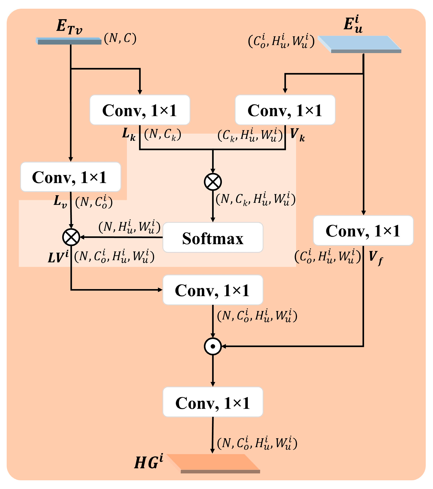
The $E_u^i$ only represents visual features at different stages. We propose the TAM, which uses text information to guide the alignment of visual and text features. This alignment helps adaptively enhance the multi-scale visual features of different classes.

As shown in Figure 2, $E_{Tv}$ is first projected into both the language value space $L_v\in {ℝ}^{N\times C_o^i}$ and language key space $L_k\in {ℝ}^{N\times C_k}$. These projections facilitate the feature matching and alignment process. At the same time, $E_u^i$ is projected onto the visual-query space $V_k^i\in {ℝ}^{C_k\times H_u^i\times W_u^i}$, which is used for computing attention maps, and the visual projection space $V_f^i\in {ℝ}^{C_o^i\times H_u^i\times W_u^i}$, which is used for feature recovery. An attention mechanism is then constructed to calculate the similarity between the $V_k^i$ and the $L_k$. The $L_v$ is weighted to obtain the weighted visual–language fusion feature $L{V}^i\in {ℝ}^{N\times C_o^i\times H_u^i\times W_u^i}$. Finally, convolutional layers are used to further fuse $L{V}^i$ and $V_f^i$, generating a multimodal aligned hierarchical guidance feature $H{G}^i\in {ℝ}^{N\times C_o^i\times H_u^i\times W_u^i}$.

The number of channels $C_k$ after visual and language projection will have an impact on the performance of the module. In subsequent experiments, if not explicitly stated, $C_k$ = 512.

3.4.2. Hierarchical Guidance Upsampling Module

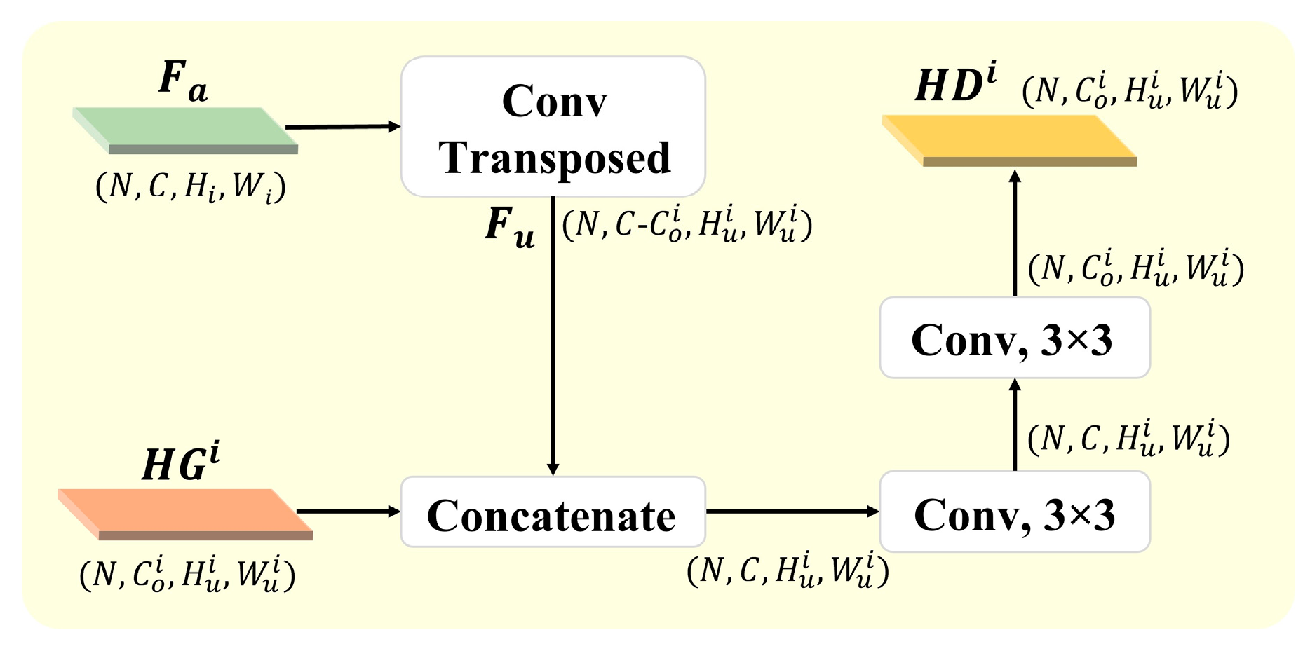
The HGU module achieves feature upsampling and multi-level feature fusion through guided features. As shown in Equation (5), the input for the first stage is $F_a$, and for subsequent stages, the input is the output from the previous stage $H{D}^{i-1}$.

$$H{D}^i=\left\{\begin{array}{l}HGU\left(F_a, H{G}^i\right),i=1\hfill \\ HGU\left(H{D}^{i-1}, H{G}^i\right),i>1\hfill \end{array}\right., i=1,2\dots n$$

(5)

where $H{D}^i$ represents the $i$-th hierarchical decoder feature, and $n$ is the number of hierarchical guidance features.

We take $i$ = 1 as an example to describe the HGU module. In other cases, replace $F_a$ with $H{D}^{i-1}$. As shown in Figure 3, in order to ensure the correct concatenation of guidance features and maintain the same number of channels, the $F_a$ is first deconvoluted to reduce the number of channels and upsample the feature map to the required spatial dimensions, resulting in $F_u\in {ℝ}^{N\times (C-C_o^i)\times H_u^i\times W_u^i}$. Then, the $F_u$ is concatenated with the guidance feature $H{G}^i$ along the channel dimension to fused feature. Finally, channel information fusion and transformation are performed through two 3 × 3 convolution layers to generate the final hierarchical decoding feature $H{D}^i\in {ℝ}^{N\times C_o^i\times H_u^i\times W_u^i}$.

During the entire process, the number of channels for guiding features $C_o$ is a custom parameter. In subsequent experiments, if not explicitly stated, then $C_o$ = [128, 64], and the number of hierarchical guidance features is $n$ = 2.

4. Experimental

4.1. Datasets

To comprehensively evaluate the performance of our proposed framework on various remote sensing semantic segmentation datasets, we conducted experiments on several representative publicly available datasets. In the subsequent experiments of this section, we selected the training set of the Globe230k dataset to train our model, while the validation sets from the other datasets were utilized for model evaluation. All datasets only use three bands: Red, Green, and Blue. We preprocessed these datasets by labeling all background classes as 0 and excluded them from both the loss function and evaluation metric calculations. The following is an introduction to these datasets:

(1)

ISPRS Potsdam dataset (https://www.isprs.org/resources/datasets/benchmarks/UrbanSemLab/Default.aspx (accessed on 9 December 2024)): It is a typical historical city with large architectural complexes, narrow streets, and dense settlement structures. It consists of 38 remote sensing images with a spatial resolution of 0.05 m, each with a size of 6000 × 6000 pixels. These images were cropped into 512 × 512 patches with an overlap of 128 pixels. The dataset includes six classes: impervious surfaces, building, low vegetation, tree, car, and background. For training, we used images with IDs: 2_10, 2_11, 2_12, 3_10, 3_11, 3_12, 4_10, 4_11,4_12, 5_10, 5_11, 5_12, 6_10, 6_11, 6_12, 6_7,6_8, 6_9, 7_10, 7_11, 7_12, 7_7, 7_8, 7_9; the remaining 14 images were used for testing.

(2)

LoveDA dataset [54]: It is a land cover domain-adaptive semantic segmentation dataset that contains 5987 high-resolution images from three different cities and rural areas: Nanjing, Guangzhou, and Wuhan. It has multi-scale objects, complex backgrounds, and inconsistent class distributions. The images have a resolution of 0.3 m and are sized 1024 × 1024 pixels. During preprocessing, these images were cropped into non-overlapping patches of 512 × 512 pixels. The dataset contains seven classes: buildings, road, water, barren, forest, agriculture, and background. This dataset has default dataset splitting criteria.

(3)

GID Large dataset [55]: It is a large-scale land cover dataset constructed from Gaofen-2 satellite images, offering extensive geographic coverage and high spatial resolution. It consists of 150 images with a size of 7200 × 6800 pixels, which we cropped into non-overlapping patches of 512 × 512 pixels. The dataset includes six classes: built up, farmland, forest, meadow, water, and background. We selected 30 images for validation, and the remaining 120 images were used for training.

(4)

Globe230k dataset [56]: It is a large-scale global land cover-mapping dataset, which has three significant advantages: large scale, diversity, and multimodality. It contains 232,819 annotated images, each of size 512 × 512 pixels, with a spatial resolution of 1 m. The dataset comprises eleven classes: cropland, forest, grass, shrubland, wetland, water, tundra, impervious, bareland, ice, and background. This dataset has default dataset splitting criteria.

(5)

FLAIR #1 dataset [57]: It is a part of the dataset currently used at IGN to establish the French national land cover map reference, and includes 50 different spatial domains with high spatiotemporal heterogeneity. It consists of 77,412 remote sensing images with a spatial resolution of 0.2 m, all 512 × 512 pixels in size. The dataset contains thirteen classes of labels: building, pervious surface, impervious surface, bare soil, water, coniferous, deciduous, brushwood, vineyard, herbaceous vegetation, agricultural land, plowed land, and background. This dataset has default dataset splitting criteria.

(6)

OpenEarthMap dataset [58]: It is a global benchmark for high-resolution land cover mapping, including a mixed image set taken from different platforms. It covers 97 regions in 44 countries across 6 continents, with a spatial resolution ranging from 0.25 m to 0.5 m. During preprocessing, the images were cropped to 512 × 512 pixels. The dataset includes nine classes: bareland, rangeland, developed space, road, tree, water, agriculture land, building, and background. This dataset has default dataset splitting criteria.

(7)

LandCover.ai dataset [59]: It is an aerial image dataset covering 216.27 km² of rural areas in Poland, with a spatial resolution ranging from 0.25 m to 0.5 m. During preprocessing, the images were cropped to 512 × 512 pixels. The dataset includes five classes: buildings, woodlands, water, roads, and background. This dataset has default dataset splitting criteria.

4.2. Implementation Details

All code is implemented based on the PyTorch 1.8.0 deep learning framework and enhanced through the mmsegmentation library. We trained the model using 4 images per batch on 4 NVIDIA GeForce RTX 4090 D 24G GPUs. The AdamW optimizer with weight decay was employed, with an initial learning rate of 0.00002 and weight decay of 0.0001. We adopted the “poly” polynomial learning rate strategy, the formula being as follows: $lr=bas\mathrm{e}\_lr\times {\left(1-{\displaystyle \frac{iteration}{max\_iteration}}\right)}^{pow\mathrm{e}r}$, where $bas\mathrm{e}\_lr$ represents the initial learning rate, $iteration$ represents the current iteration number, $max\_iteration$ is the total number of iterations, and $pow\mathrm{e}r$ is set to 0.9. The maximum number of iterations was set to 80k. During the training process, we used random scaling with scales of [0.5, 0.75, 1.0, 1.25, 1.5, 1.75, 2.0], random cropping, and random flipping for data augmentation. The cross-entropy loss function was used for training. It should be noted that in subsequent experiments, unless otherwise specified, the ViT-L/14 architecture was used as the default image encoder, and the 7th and 15th layers were selected for hierarchical guidance.

4.3. Evaluation Metrics

Based on previous research on traditional semantic segmentation and OVSS, we used the mean intersection over union ($mIoU$) as the evaluation metric on a single dataset and the $meanmIoU$ as the evaluation metric on multiple datasets. The $meanmIoU$ can reflect the overall effectiveness of the proposed framework from a holistic perspective. The $mIoU$ and $meanmIoU$ are calculated as follows:

$$mIoU={\displaystyle \frac{1}{N}}{\displaystyle \sum }_{k=1}^{N}Io{U}_k={\displaystyle \frac{1}{N}}{\displaystyle \sum }_{k=1}^N{\displaystyle \frac{T{P}_k}{T{P}_k+F{P}_k+F{N}_k}}$$

(6)

$$mean mIoU={\displaystyle \frac{1}{M}}{\displaystyle \sum }_{i=1}^{M}mIo{U}_i$$

(7)

where $T{P}_k$, $F{P}_k$, $T{N}_k$, and $F{N}_k$ denote true positives, false positives, true negatives, and false negatives, respectively, for a particular object indexed as category k. N is the number of classes, M is the number of datasets used.

4.4. Comparison with State-of-the-Art Methods

We compare the proposed HG-RSOVSSeg with several state-of-the-art OVSS methods, including LSeg [44], Fusioner [45], SAN [46], and Cat-Seg [25]. These methods are publicly available, and represent the latest advancements in OVSS in computer vision, demonstrating excellent segmentation performance. Since previous studies have not applied these methods to remote sensing tasks, we followed their original configurations to train and test them under the same experimental conditions as our proposed method. According to their original configuration, except for the Cat-Seg, which fine-tunes the encoder’s attention layer, the encoders of all other methods were kept frozen.

Table 1. Comparison of experiment results with state-of-the-art methods. The best results are in bold. $mIoU$ and mean mIoU are represented as percentages (%).

Method	$\mathit{m}\mathit{I}\mathit{o}\mathit{U}$						mean mIoU	FLOPs (T)	Params (G)
	Potsdam	LoveDA	GID Large	FLAIR #1	OpenEarthMap	LandCover.ai
LSeg	20.18	31.99	61.50	15.09	28.72	55.33	35.47	1.246	0.551
Fusioner	19.05	36.11	56.49	13.91	26.35	56.20	34.69	1.078	0.462
SAN	11.72	24.16	40.60	10.24	17.74	53.43	26.32	1.066	0.436
Cat-Seg	17.59	34.48	39.81	19.77	19.28	46.05	29.50	1.022	0.433
HG-RSOVSSeg (Ours)	22.85	36.15	67.63	12.54	27.74	57.71	37.44	1.036	0.433

presents the quantitative evaluation results of different methods on six datasets. As can be seen, our proposed method achieved the highest $mIoU$ values on the Potsdam, LoveDA, GID Large, and LandCover.ai datasets. LSeg and SAN attained the highest and lowest $meanmIoU$ values, 35.47% and 26.32%, respectively, with our method outperforming them by 1.97% and 11.12%, respectively. In addition, we evaluated the floating point operations (FLOPs) and parametric quantities (Params) of each method, and the results are shown in Table 1. Cat-Seg has the lowest FLOPs and Params, and our method follows closely behind. Notably, while the Params remain consistent, the proposed method achieves a 7.94% improvement in $meanmIoU$ with an increase of only 0.014 T in FLOPs.

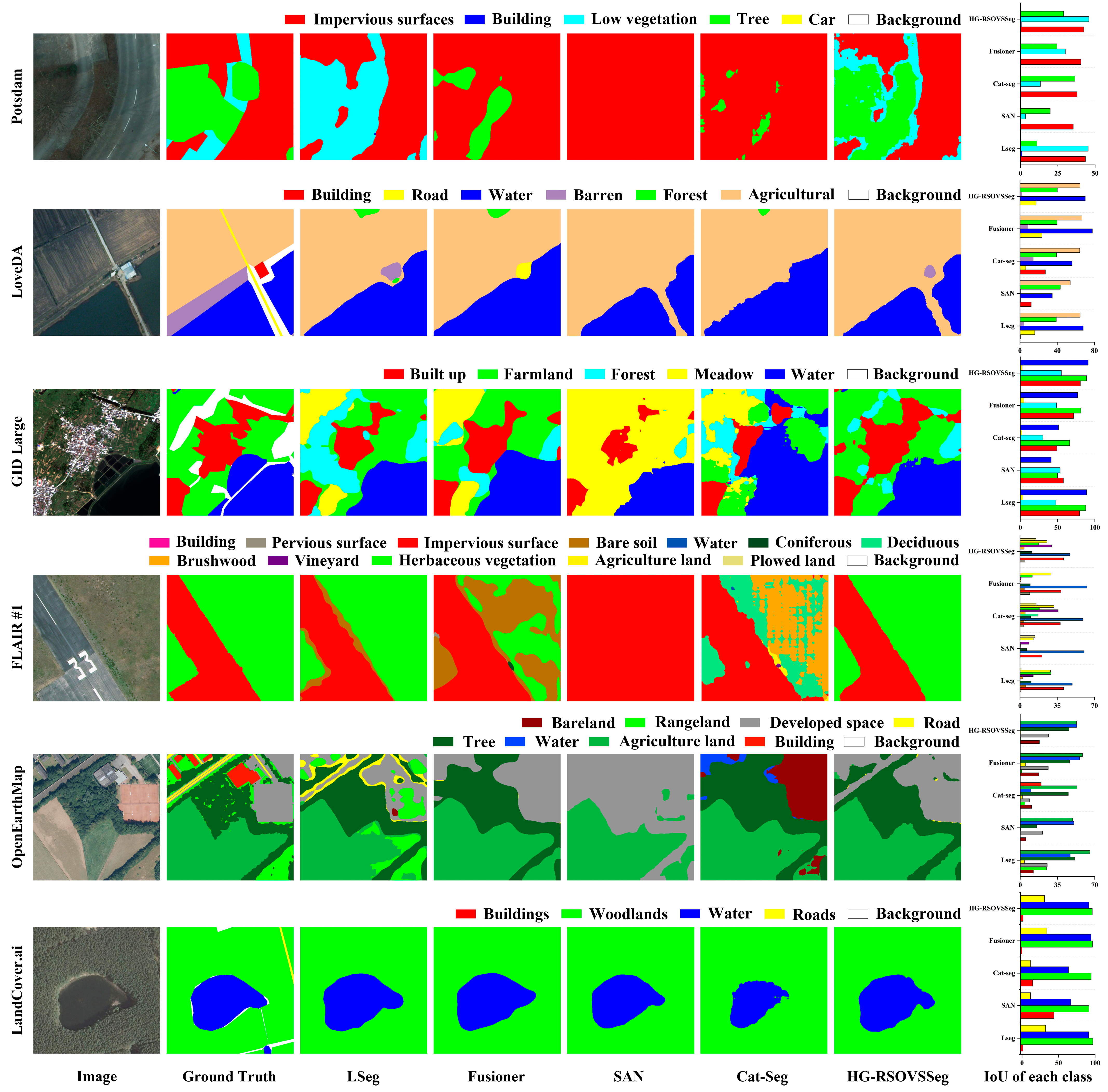
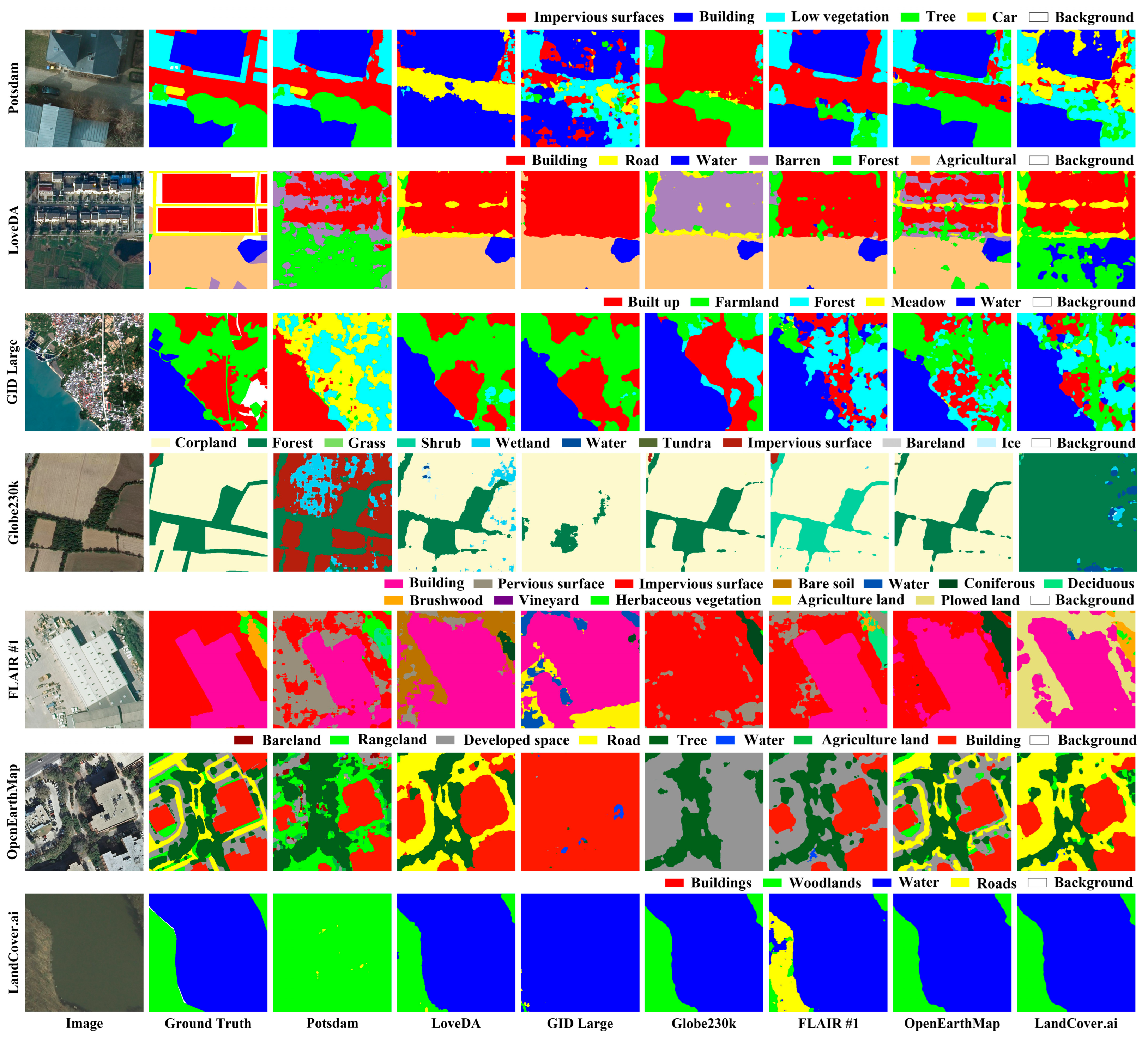
Figure 4 shows the visualization results of different methods on six datasets, and the bar charts of $IoU$ for each class in each dataset. It can be seen that within the same dataset, the $IoU$ distributions of each class across different models have similarity. For classes that appear in the training set (e.g., water, forest, and impervious surface), the prediction accuracy is relatively high across all models. Moreover, our method demonstrates strong performance in predicting previously unseen classes, such as low vegetation and tree in the Potsdam dataset, agricultural in the LoveDA dataset, built-up and farmland in the GID Large dataset, vineyard and agricultural land in the FLAIR #1 dataset, tree and developed space in OpenEarthMap dataset, and woodlands and roads in the LandCover.ai dataset. These results further demonstrate the feasibility of using pre-trained VLMs for OVSS tasks in remote sensing.

Although the proposed HG-RSOVSSeg achieves competitive or superior performance on most benchmarks, its performance on the FLAIR #1 and OpenEarthMap datasets is relatively lower compared with some existing approaches. Based on the bar charts of $IoU$ for each class in each dataset in Figure 4, we further analyze the categories that contribute most to the performance gap on different datasets. For the FLAIR #1 dataset, deciduous and water are identified as the primary contributors to the performance difference between our method and the best-performing baseline. Similarly, for the OpenEarthMap dataset, rangeland and agricultural land are the main classes responsible for the observed performance gap. These differences are closely related to the feature fusion strategies adopted by different methods. LSeg and Fusioner adopt a strategy of decoding followed by fusion, with the latter increasing the depth processing of text features. Cat-Seg adopts a strategy of fusion before decoding, while SAN adds external adapters for feature fusion. Our method uses a decoding and fusion hierarchical embedding strategy.

Overall, all models performed the worst on the FLAIR #1 dataset. This is mainly because FLAIR #1 contains a large number of fine-grained land cover classes, which are difficult to distinguish using single class-name embeddings. Moreover, the scenes in FLAIR #1 are highly complex, with dense object distributions and frequent co-occurrence of multiple land cover types, further increasing the difficulty of discriminating semantically related classes in the open-vocabulary setting.

4.5. Parameter Analysis

4.5.1. Effect of Different $C_k$ in TAM

We conducted experiments to assess the impact of the number of channels ($C_k$) after visual and text projection on model performance. Specifically, $C_k$ was set to 256, 512, and 1024, while the encoder was frozen, and $C_o$ was set to [128, 64]. All other parameters and settings remain unchanged. As $C_k$ decreases, the model learns fewer features, whereas an increase in $C_k$ results in a larger number of parameters to be calculated. As shown in Figure 5a, the performance of the model is best when $C_k$ is set to 512. When the value increases or decreases, the performance of the model will decrease by about 2%.

4.5.2. Effect of Different $C_o$ in HGU

In image encoders, intermediate features preserve more structural and boundary information, while deeper features encode higher-level semantic concepts. Using moderate channel dimensions allows the decoder to balance semantic expressiveness and computational efficiency when aligning these features with text embeddings. We analyzed the effect of the number of channels ($C_o$) of the guidance features in the HGU module, which is consistent with the number $n$ of guidance features. We tested various configurations: for $n$ = 2, we used $C_o$= [64, 32], [128, 64], [256, 128], and for $n$ = 3, $C_o$ = [256, 128, 64], with the corresponding guidance layers set to [7, 15] and [5, 11, 17], respectively. In all experiments, the encoder was frozen, and $C_k$ was set to 512, and all other parameters and settings remain unchanged. As shown in Figure 5b, the optimal model performance is achieved when $n$ = 2 and $C_o$ = [128, 64], followed by the $n$ = 3 and $C_o$ = [256, 128, 64]. Increasing the number of guidance features beyond two does not yield further improvements and slightly degrades performance. This is mainly due to the characteristics of ViT-based encoders, where intermediate- and final-stage features share the same spatial resolution. Applying guidance to earlier stages requires large upsampling factors during decoding, which degrades the semantic quality of the guidance features and amplifies noise. Consequently, excessive hierarchical guidance becomes less informative while increasing computational cost.

4.5.3. Effect of Different Numbers of Training Samples

Remote sensing semantic segmentation often suffers from limited annotated data due to the high cost of pixel-level labeling. To evaluate the effectiveness of the proposed method under data-scarce conditions, we randomly selected 10%, 30%, and 50% of the training data from the Globe230k dataset for training and conducted inference on the same test set. The quantitative results are shown in Figure 5c. When only 10% of the training samples are used, the model still achieves a $meanmIoU$ of 32.00%, and the performance consistently improves as more training data become available. Notably, the performance gap between using 50% and 100% of the training data is relatively small, indicating that the model can effectively leverage the pre-trained vision–language representations to mitigate the reliance on large-scale annotated datasets.

4.5.4. Effect of Different Templates in Text Encoder

When encoding class labels in a dataset, the text encoder needs to pre-construct sentences for each class label. Different construction templates may have an impact on the model performance. We conducted experimental analysis on the three most commonly used templates: “vild”, “imagenet”, and “imagenet_select_clip” [43,46]. For completeness and reproducibility, the detailed sentence templates are provided in the Supplementary Materials. The “imagenet” templates are mainly object-centric and emphasize instance-level appearance attributes, which are effective for natural images but less aligned with remote sensing land cover classes that are typically region-based. Although the “imagenet_select_clip” templates introduce scene-level expressions, they still implicitly assume discrete and maskable objects, limiting their effectiveness for large-scale and continuous land cover regions. In contrast, the “vild” templates are explicitly scene-oriented and region-aware, using existence-based descriptions without introducing appearance-specific noise. This design better matches the semantic characteristics of land cover classes in high-resolution remote sensing images. As shown in

Table 2. Comparison of experimental results under different templates. $mIoU$ and mean mIoU are represented as percentages (%).

Templates	Number	$\mathit{m}\mathit{I}\mathit{o}\mathit{U}$						mean mIoU
		Potsdam	LoveDA	GID Large	FLAIR #1	OpenEarthMap	LandCover.ai
vild	14	23.53	32.36	63.58	16.28	24.70	55.01	35.91
imagenet_select_clip	32	22.27	29.76	63.24	15.51	25.18	54.98	35.16
imagenet	80	24.02	34.23	65.06	14.98	23.34	53.97	35.93

, despite using significantly fewer templates, “vild” achieves comparable performance across multiple datasets. This indicates that semantically consistent and task-aligned prompts are more effective than a large number of heterogeneous templates. Moreover, we found that as the number of template sentences gradually increased, the time required to encode class labels also increased, leading to the model computation time correspondingingly increasing significantly.

4.6. Ablation Study

To validate the contributions of each module in the proposed framework, we conducted extensive ablation experiments.

Table 3. The results of ablation experiments. $\mathrm{mIoU}$ and mean mIoU are represented as percentages (%).

PEA	FA	HD		$\mathit{m}\mathit{I}\mathit{o}\mathit{U}$						mean mIoU
		HGU	TAM	Potsdam	LoveDA	GID Large	FLAIR #1	OpenEarthMap	LandCover.ai
✓	✓			14.37	24.81	45.56	12.32	19.10	50.91	27.85
✓	✓	✓		15.50	33.53	55.85	14.11	25.18	56.67	33.47
✓	✓	✓	✓	23.53	32.36	63.58	16.28	24.70	55.01	35.91
	✓	✓	✓	21.94	33.55	61.70	15.50	25.42	54.62	35.46

presents the detailed results of the ablation experiments on the PEA strategy, TAM, and HGU module.

When the image size is fixed at 512 and the PEA strategy and FA module are used, adding the HGU module can increase the $meanmIoU$ value by about 5.6%. Further addition of the TAM can increase the performance by about 2.4%. Meanwhile, the $mIoU$ values increase gradually with the increase in modules on different datasets, which has led to a certain degree of improvement. This indicates that our proposed modules contribute significantly to enhancing the model performance, especially the TAM. We conducted experiments on two configurations to evaluate the impact of the PEA strategy: (i) directly interpolating the image to a size of 224 without using PEA, and (ii) fine-tuning the weights of positional embeddings while using PEA. It can be seen that using the PEA strategy has an improvement of about 0.5% in model performance compared to not using it. Different feature aggregation methods can have a certain impact on model performance. We compared the proposed FA module with two other aggregation methods, namely traditional aggregation and cost aggregation [25], and the results are shown in

Table 4. Comparison of experimental results under different feature aggregation methods. The best results are in bold. $mIoU$ and mean mIoU are represented as percentages (%).

$\mathit{F}\mathit{A}$	$\mathit{m}\mathit{I}\mathit{o}\mathit{U}$						mean mIoU
	Potsdam	LoveDA	GID Large	FLAIR #1	OpenEarthMap	LandCover.ai
Similarity-based	21.26	29.09	63.36	14.56	24.36	51.07	33.95
Cost	18.78	32.04	66.25	14.51	22.13	53.83	34.59
Ours	23.53	32.36	63.58	16.28	24.70	55.01	35.91

. The $meanmIoU$ of our proposed FA module outperforms the other two methods. The performance of similarity-based fusion is the worst.

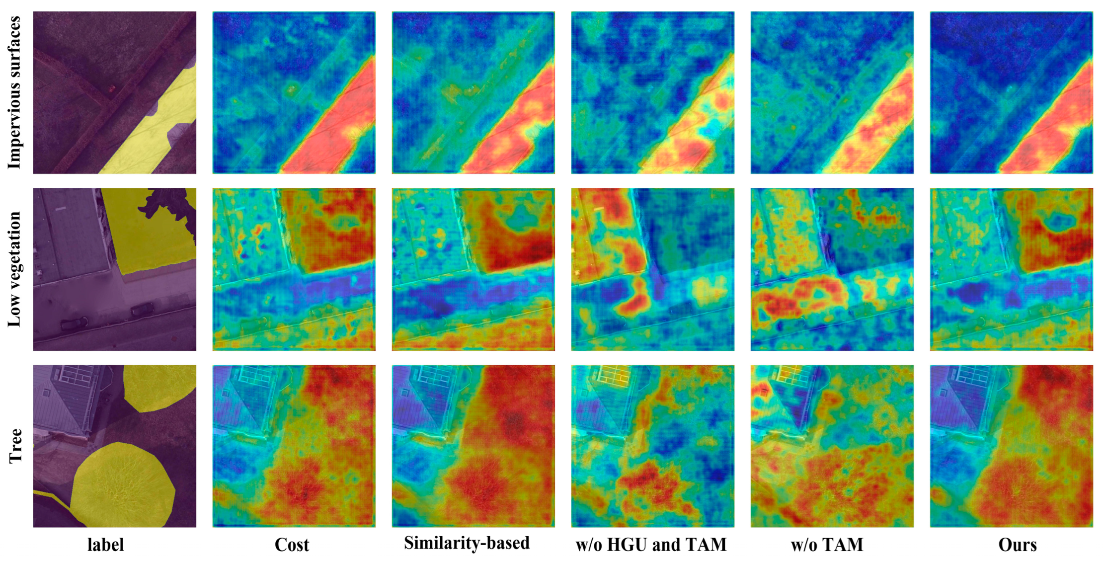
As shown in Figure 6, we visualized the feature maps of three different feature aggregation strategies and ablation studies of the HD module. Compared with the cost-based and similarity-based aggregation methods, our proposed FA module exhibits significantly more compact and coherent response regions, with clear boundaries. This indicates that our method provides more discriminative feature representations, enabling accurate perception of semantic boundaries and internal class structures. When both the HGU and TAM are removed, the feature responses become very coarse and scattered. After adding the HGU module, the spatial distribution of the features becomes more continuous, the semantic distinction between classes is enhanced, and the object boundaries are better preserved. With the further addition of the TAM, the model is able to more effectively highlight task-relevant regions and suppress background noise. For instance, in the “low vegetation”, non-vegetation areas are significantly attenuated, with responses concentrated on the target regions. These results demonstrate that the HGU module can help the model understand complex spatial structures and contextual information, while the TAM enables the model to focus on key areas of the current semantic task.

5. Discussion

5.1. Comparison of the Different Pre-Trained VLMs and Frozen Stages

In this section, we compare the performance of different pre-trained VLMs and explore the effects of different frozen stages.

Table 5. The experiment results of different pre-trained VLMs and frozen stages. The best results are in bold. $mIoU$ and mean mIoU are represented as percentages (%).

Pre-Trained VLMs	Frozen Stages		$\mathit{m}\mathit{I}\mathit{o}\mathit{U}$						mean mIoU	Globe230k
	Image Encoder	Text Encoder	Potsdam	LoveDA	GID Large	FLAIR #1	OpenEarthMap	LandCover.ai
CLIP ViT-L/14	✓	✓	23.53	32.36	63.58	16.28	24.70	55.01	35.91	68.31
CLIP ViT-L/14		✓	19.63	33.13	66	14.07	26.01	55.2	35.67	74.95
CLIP ViT-L/14	✓		19.17	27.02	22.53	9.75	9.04	50.57	23.1	68.57
CLIP ViT-L/14			13.47	19.44	20.78	9.01	9.86	46.83	19.90	74.82
CLIP ViT-B/16	✓	✓	17.09	30.86	60.95	14.57	19.31	46.62	31.57	-
CLIP ViT-B/32	✓	✓	16.43	28.4	47.32	12.41	13.06	47.94	27.59
CLIP ViT-L/14@336	✓	✓	24.01	31.39	65.66	15.7	25.25	55.69	36.28
RemoteCLIP ViT-B/32	✓	✓	10.31	18.03	50.34	12.09	14.06	50.46	25.88
RemoteCLIP ViT-L/14	✓	✓	16.42	27.48	65.6	14.9	17.1	55.29	32.80
GeoRSCLIP ViT-B/32	✓	✓	20.01	31.87	44.24	12.82	12.79	52.01	28.96
GeoRSCLIP ViT- L/14	✓	✓	22.77	34.61	67.5	14.46	25.83	58.71	37.31
GeoRSCLIP ViT-L/14@336	✓	✓	22.85	36.15	67.63	12.54	27.74	57.71	37.44
SkyCLIP ViT- B/32	✓	✓	6.25	27.44	39.27	11.79	14.32	50.27	24.89
SkyCLIP ViT-L/14	✓	✓	25.63	31.05	62.03	14.96	24.08	55.74	35.58

shows the experimental results.

In the experiments with different frozen stages, we use the CLIP ViT-L/14 pre-trained framework and ensured that other parameters were consistent. The experiments were conducted on whether to freeze image and text encoders. It should be noted that the “unfrozen” mentioned in this section refers to fine-tuning the attention and positional embedding layers, which is superior to other methods in terms of efficiency and accuracy. The experimental results indicate that fine-tuning the encoder can lead to varying degrees of performance degradation, with text encoder fine-tuning resulting in a more significant drop in performance compared to fine-tuning the image encoder. This is due to the contrastive-learning mechanism used in the pre-trained CLIP, where images and their corresponding text descriptions have consistent. Fine-tuning the text encoder disrupts this consistency, resulting in a catastrophic decline in performance. In contrast, fine-tuning the image encoder can significantly improve prediction accuracy for the same dataset.

We compared four architectures of pre-trained CLIP models: ViT-B/16, ViT-B/32, ViT-L/14, and ViT-L/14@336. Meanwhile, we also compare several other pre-trained VLMs specifically in remote sensing, including RemoteCLIP, GeoRSCLIP, and SkyCLIP. These models provide ViT-B/32 and ViT-L/14 architectures, with GeoRSCLIP also providing ViT-L/14@336 architecture. After freezing these VLMs, we conducted experiments using the same experimental settings. Table 5 shows that the ViT-L/14@336 architecture from GeoRSCLIP outperforms the others, achieving the highest $meanmIoU$ of 37.44%. Under the same pre-trained VLMs, the $meanmIoU$ of ViT-L/14 is higher than that of ViT-B/16 and ViT-B/32, with a significant improvement. The performance difference between ViT-L/14 and ViT-L/14@336 is not significant.

5.2. Influence of Different Training Datasets on Model Performance

Due to inherent differences in data acquisition methods, spatial resolution, and acquisition scenarios across these datasets, the performance varies significantly on each dataset. In this section, we conducted statistical analysis of the band distribution and spatial resolution of each dataset, as shown in Figure 7. Meanwhile, the model is trained individually using the training set of each dataset, the test set of all datasets is evaluated, and the experimental results are summarized in

Table 6. The experiment results of the different training datasets. $mIoU$ and mean mIoU are represented as percentages (%). The best results are in bold. Gray represents the $mIoU$ value of the training set used on the corresponding test set, which is not included in the calculation of $meanmIoU$.

Training Dataset	$\mathit{m}\mathit{I}\mathit{o}\mathit{U}$							mean mIoU
	Potsdam	LoveDA	GID Large	Globe230k	FLAIR #1	OpenEarthMap	LandCover.ai
Potsdam	80.78	9.27	10.99	7.85	14.41	18.23	33.31	15.68
LoveDA	10.18	64.56	51.98	18.63	14.37	28.41	72.72	32.72
GID Large	22.65	37.25	95.22	18.38	7.32	21.21	56.86	27.28
Globe230k	22.85	36.15	67.63	69.25	12.54	27.74	57.71	37.44
FLAIR #1	41.83	43.14	37.25	23	59.82	25.36	75.8	41.06
OpenEarthMap	39.59	62.58	58.21	28.02	14.92	62.56	87.23	48.43
LandCover.ai	26.86	33.71	30.13	11.63	12.16	19.45	94.2	36.09

. The visualization results on seven datasets are shown in Figure 8. For these experiments, we used the GeoRSCLIP ViT-L/14@336 with optimal performance as the pre-trained VLM, $C_k$ = 512, $C_o$ = [128, 64], selecting the “vild” templates as the construction template, and freezing the encoder stage.

Based on the experimental results, we found that the model trained on the OpenEarthMap dataset achieved the best performance, with a $meanmIoU$ of 48.43%. In contrast, the model trained on the Potsdam dataset had the lowest $meanmIoU$ of 15.68%, a difference of 32.75%. This is because the Potsdam dataset is a high-resolution aerial image dataset with a spatial resolution of 0.05 m, meaning that many features are more prominent and have larger scales. The spatial resolution of the other datasets is at the decimeter level, and the difference in spatial resolution is the main reason for the poor performance using the Potsdam dataset for training. The OpenEarthMap dataset, which consists of mixed images captured by different platforms, offers a more balanced data distribution with a spatial resolution ranging from 0.25 to 0.5 m. As a result, models trained on this dataset perform exceptionally well.

Both spatial resolution and band distribution are critical factors influencing the performance of OVSS tasks. When data distributions differ significantly, the prediction accuracy can still be considerably low even if the spatial resolutions are similar. For example, the LandCover.ai and OpenEarthMap datasets have comparable spatial resolutions, but the former has a more concentrated data distribution, while the latter has a more uniform distribution. As a result, models trained on the LandCover.ai dataset show poor performance when applied to the OpenEarthMap dataset, while models trained on the OpenEarthMap dataset show strong performance on the LandCover.ai dataset. Similarly, when band distributions are comparable, moderate differences in spatial resolution can still impact predictive accuracy. For example, the FLAIR #1 and OpenEarthMap datasets have a similar band distribution, but the significantly different spatial resolutions of the two datasets result in lower accuracy for the FLAIR #1 dataset compared to the OpenEarthMap dataset. Additionally, although the OpenEarthMap and LoveDA datasets have a slightly lower band similarity, their comparable spatial resolutions contribute to relatively high prediction accuracy between them. In conclusion, OVSS tasks based on pre-trained VLMs show strong applicability and generalization, particularly when the spatial resolutions of the images are similar and the band distributions do not differ significantly.

In addition, semantic granularity and ambiguity of class names also contribute to the observed performance differences across datasets. The FLAIR #1 dataset contains more fine-grained land cover classes, many of which are conceptually related or partially overlapping. When such classes are represented solely by single class names, their corresponding text embeddings may become highly similar, resulting in ambiguous text-to-pixel alignment. Moreover, the same land cover type may be described using different class names across datasets, leading to inconsistent text embeddings for semantically similar classes. This inconsistency further amplifies performance variations in the OVSS setting, where segmentation results are highly sensitive to the quality and distinctiveness of text representations.

5.3. Limitations and Future Works

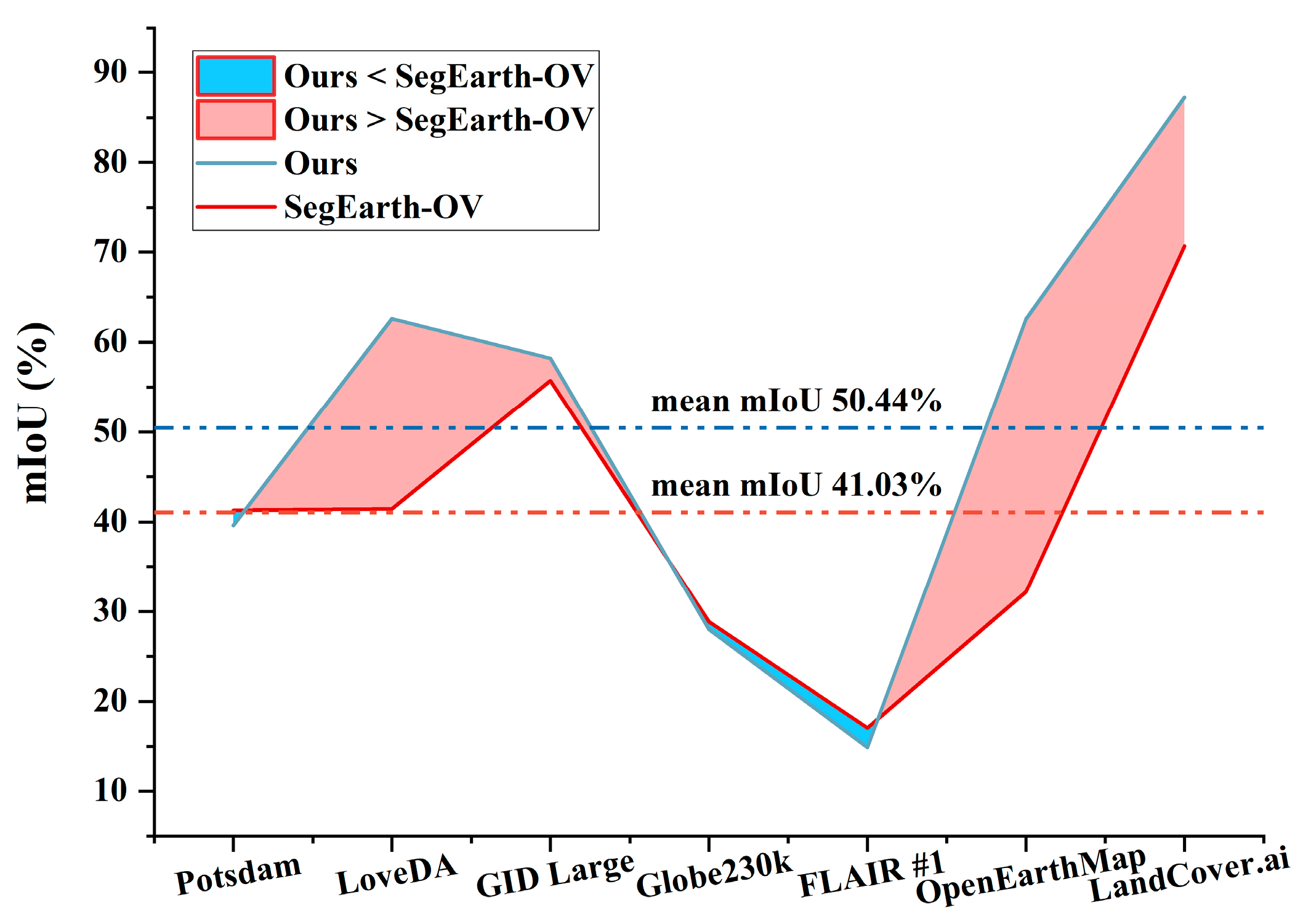
The method proposed in this paper requires supervised training of the FA module and the HD on a semantic segmentation dataset in advance. This provides greater flexibility but also imposes a constraint in terms of dataset dependency. Based on the experimental analysis in Section 5.2, we recommend using the OpenEarthMap dataset as the training set, and other datasets as the testing set for evaluating the performance of OVSS tasks in the remote sensing field in future studies. Currently, SegEarth-OV [49] is the most famous OVSS work in the field of remote sensing. This method requires pre-training on a small set of unlabeled image data, and the entire training process is independent of the semantic-segmentation task itself. The trained weights can be used for a wide range of remote sensing data. Figure 9 shows the $mIoU$ values of our method and SegEarth-OV on seven datasets. It can be seen that our method outperforms or matches SegEarth-OV on all datasets, achieving an overall $meanmIoU$ improvement of 9.4%.

There are limitations in using the CLIP model for semantic-segmentation tasks, as it was not specifically designed for this purpose. Although the decoder design in this paper can alleviate this problem to some extent, its segmentation effect is not good in certain cases. The SAM model has robust generalization in image-segmentation tasks, but it lacks the semantic information required for high-quality segmentation in remote sensing. A promising direction for future work would be to combine the advantages of both models: using CLIP to provide semantic information and point prompts for SAM, thereby enhancing the segmentation accuracy of SAM while using the semantic guidance from CLIP.

Additionally, previous studies on semantic segmentation often used a single vocabulary to represent classes, which is converted into numerical values (e.g., 0-n) for loss computation. The OVSS requires the text encoder to process class names and generate corresponding text embeddings. The accuracy of these text embeddings directly affects the performance of the model. In remote sensing applications, many land cover classes exhibit one-to-many or many-to-one relationships. For example, the “building” should include “roof” and “house”, while the “water” should also include “river” and “lake”. Furthermore, the class labels in remote sensing have diverse characteristics, and labeling criteria between different remote sensing datasets are often inconsistent, which introduces additional complexity. Recent studies [52,60,61] have shown that using synonyms or richer class descriptions as text inputs has been demonstrated to be beneficial, as they provide additional semantic cues beyond single class names. A promising direction for further addressing this issue is to combine remote sensing land cover knowledge graphs to provide a more structured and hierarchical embedding of text information, thereby addressing these inconsistencies and improving the performance of OVSS in remote sensing.

6. Conclusions

In this paper, we propose a multimodal framework named HG-RSOVSSeg, which utilizes the advantages of text–image feature alignment in CLIP to hierarchically integrate remote sensing semantic class information and image features, thereby enhancing semantic segmentation performance under open classes. The proposed PEA strategy enables the model to generalize effectively to inputs of different sizes by interpolating position embeddings. Additionally, the FA module ensures efficient pixel-level alignment and interaction between text and visual features. Guided by text-feature alignment, the HD generates more accurate and comprehensive representations, significantly improving the segmentation quality and producing high-resolution, fine-grained outputs. To evaluate the effectiveness of HG-RSOVSSeg, we conducted extensive experiments on six representative remote sensing image semantic segmentation datasets. The experimental results demonstrate that our proposed framework substantially outperforms state-of-the-art methods, and all proposed modules have achieved good performance. Moreover, we conducted in-depth experimental analysis on the impact of template construction, pre-trained models, and changes in training data on model performance, revealing their potential mechanisms and providing suggestions for future research. While the pre-trained VLMs hold great promise for free-form segmentation of remote sensing images, several challenges remain. In future work, we aim to address the limitations of existing approaches by incorporating knowledge graphs and advanced remote sensing specific large-model technologies, ultimately achieving more accurate and robust free-form semantic segmentation for remote sensing images.

References

1. Cheng, J.; Deng, C.; Su, Y.; An, Z.; Wang, Q. Methods and datasets on semantic segmentation for Unmanned Aerial Vehicle remote sensing images: A review. ISPRS J. Photogramm. Remote Sens. 2024, 211, 1–34. [Google Scholar] [CrossRef]
2. Zhang, X.; Chen, G.; Wang, W.; Wang, Q.; Dai, F. Object-Based Land-Cover Supervised Classification for Very-High-Resolution UAV Images Using Stacked Denoising Autoencoders. IEEE J. Sel. Top. Appl. Earth Obs. Remote Sens. 2017, 10, 3373–3385. [Google Scholar] [CrossRef]
3. Zhu, Q.; Lei, Y.; Sun, X.; Guan, Q.; Zhong, Y.; Zhang, L.; Li, D. Knowledge-guided land pattern depiction for urban land use mapping: A case study of Chinese cities. Remote Sens. Environ. 2022, 272, 112916. [Google Scholar] [CrossRef]
4. Wei, S.; Ji, S. Graph Convolutional Networks for the Automated Production of Building Vector Maps From Aerial Images. IEEE Trans. Geosci. Remote Sens. 2022, 60, 1–11. [Google Scholar] [CrossRef]
5. Hetang, C.; Xue, H.; Le, C.; Yue, T.; Wang, W.; He, Y. Segment Anything Model for Road Network Graph Extraction. In Proceedings of the IEEE/CVF Conference on Computer Vision and Pattern Recognition (CVPR), Seattle, WA, USA, 17–21 June 2024; pp. 2556–2566. [Google Scholar]
6. Yang, J.; Ding, M.; Huang, W.; Li, Z.; Zhang, Z.; Wu, J.; Peng, J. A Generalized Deep Learning-based Method for Rapid Co-seismic Landslide Mapping. IEEE J. Sel. Top. Appl. Earth Obs. Remote Sens. 2024, 17, 16970–16983. [Google Scholar] [CrossRef]
7. Huang, W.; Ding, M.; Li, Z.; Yu, J.; Ge, D.; Liu, Q.; Yang, J. Landslide susceptibility mapping and dynamic response along the Sichuan-Tibet transportation corridor using deep learning algorithms. Catena 2023, 222, 106866. [Google Scholar] [CrossRef]
8. Li, R.; Zheng, S.; Zhang, C.; Duan, C.; Wang, L.; Atkinson, P.M. ABCNet: Attentive bilateral contextual network for efficient semantic segmentation of Fine-Resolution remotely sensed imagery. ISPRS J. Photogramm. Remote Sens. 2021, 181, 84–98. [Google Scholar] [CrossRef]
9. Wang, L.; Li, R.; Zhang, C.; Fang, S.; Duan, C.; Meng, X.; Atkinson, P.M. UNetFormer: A UNet-like transformer for efficient semantic segmentation of remote sensing urban scene imagery. ISPRS J. Photogramm. Remote Sens. 2022, 190, 196–214. [Google Scholar] [CrossRef]
10. Ma, X.; Zhang, X.; Pun, M.O. RS3Mamba: Visual State Space Model for Remote Sensing Image Semantic Segmentation. IEEE Geosci. Remote Sens. Lett. 2024, 21, 6011405. [Google Scholar] [CrossRef]
11. Liu, J.; Zhang, F.; Zhou, Z.; Wang, J. BFMNet: Bilateral feature fusion network with multi-scale context aggregation for real-time semantic segmentation. Neurocomputing 2023, 521, 27–40. [Google Scholar] [CrossRef]
12. Huang, W.; Deng, F.; Liu, H.; Ding, M.; Yao, Q. Multiscale Semantic Segmentation of Remote Sensing Images Based on Edge Optimization. IEEE Trans. Geosci. Remote Sens. 2025, 63, 5616813. [Google Scholar] [CrossRef]
13. Li, Y.; Zhang, W.; Liu, Y.; Shao, X. A lightweight network for real-time smoke semantic segmentation based on dual paths. Neurocomputing 2022, 501, 258–269. [Google Scholar] [CrossRef]
14. Li, Y.; Shi, T.; Zhang, Y.; Chen, W.; Wang, Z.; Li, H. Learning deep semantic segmentation network under multiple weakly-supervised constraints for cross-domain remote sensing image semantic segmentation. ISPRS J. Photogramm. Remote Sens. 2021, 175, 20–33. [Google Scholar] [CrossRef]
15. Huang, W.; Ding, M.; Deng, F. Domain-Incremental Learning for Remote Sensing Semantic Segmentation With Multifeature Constraints in Graph Space. IEEE Trans. Geosci. Remote Sens. 2024, 62, 5645215. [Google Scholar] [CrossRef]
16. Pourpanah, F.; Abdar, M.; Luo, Y.; Zhou, X.; Wang, R.; Lim, C.P.; Wang, X.Z.; Wu, Q.M.J. A Review of Generalized Zero-Shot Learning Methods. IEEE Trans. Pattern Anal. Mach. Intell. 2023, 45, 4051–4070. [Google Scholar] [CrossRef]
17. Li, Y.; Ouyang, S.; Zhang, Y. Combining deep learning and ontology reasoning for remote sensing image semantic segmentation. Knowl.-Based Syst. 2022, 243, 108469. [Google Scholar] [CrossRef]
18. Liu, W.; Zhang, H.; Xia, X.; Wang, L.; Sun, J. Semantic-Embedded Knowledge Acquisition and Reasoning for Image Segmentation. In Proceedings of the 2023 IEEE International Conference on Image Processing (ICIP), Kuala Lumpur, Malaysia, 8–11 October 2023; pp. 2360–2364. [Google Scholar]
19. Chen, S.; Li, Z.; Yang, X. Knowledge Reasoning for Semantic Segmentation. In Proceedings of the IEEE International Conference on Acoustics, Speech and Signal Processing (ICASSP), Toronto, ON, Canada, 6–11 June 2021; pp. 2340–2344. [Google Scholar]
20. Li, Y.; Kong, D.; Zhang, Y.; Tan, Y.; Chen, L. Robust deep alignment network with remote sensing knowledge graph for zero-shot and generalized zero-shot remote sensing image scene classification. ISPRS J. Photogramm. Remote Sens. 2021, 179, 145–158. [Google Scholar] [CrossRef]
21. Chen, J.; Geng, Y.; Chen, Z.; Pan, J.Z.; He, Y.; Zhang, W.; Horrocks, I.; Chen, H. Zero-Shot and Few-Shot Learning With Knowledge Graphs: A Comprehensive Survey. Proc. IEEE 2023, 111, 653–685. [Google Scholar] [CrossRef]
22. Radford, A.; Kim, J.W.; Hallacy, C.; Ramesh, A.; Goh, G.; Agarwal, S.; Sastry, G.; Askell, A.; Mishkin, P.; Clark, J.; et al. Learning Transferable Visual Models From Natural Language Supervision. In Proceedings of the 38th International Conference on Machine Learning (ICML), Virtual Event, 18–24 July 2021; pp. 8748–8763. [Google Scholar]
23. Li, X.; Wen, C.; Hu, Y.; Zhou, N. RS-CLIP: Zero shot remote sensing scene classification via contrastive vision-language supervision. Int. J. Appl. Earth Obs. Geoinf. 2023, 124, 103497. [Google Scholar] [CrossRef]
24. Jiang, W.; Sun, Y.; Lei, L.; Kuang, G.; Ji, K. AdaptVFMs-RSCD: Advancing Remote Sensing Change Detection from binary to semantic with SAM and CLIP. ISPRS J. Photogramm. Remote Sens. 2025, 230, 304–317. [Google Scholar] [CrossRef]
25. Cho, S.; Shin, H.; Hong, S.; An, S.; Lee, S.; Arnab, A.; Seo, P.H.; Kim, S. CAT-Seg: Cost Aggregation for Open-Vocabulary Semantic Segmentation. In Proceedings of the IEEE/CVF Conference on Computer Vision and Pattern Recognition (CVPR), Seattle, WA, USA, 17–21 June 2024; pp. 4113–4123. [Google Scholar]
26. Wu, J.; Li, X.; Xu, S.; Yuan, H.; Ding, H.; Yang, Y.; Li, X.; Zhang, J.; Tong, Y.; Jiang, X.; et al. Towards Open Vocabulary Learning: A Survey. IEEE Trans. Pattern Anal. Mach. Intell. 2024, 46, 5092–5113. [Google Scholar] [CrossRef]
27. Chen, Y.-C.; Li, L.; Yu, L.; El Kholy, A.; Ahmed, F.; Gan, Z.; Cheng, Y.; Liu, J. Uniter: Universal image-text representation learning. In Proceedings of the European Conference on Computer Vision (ECCV), Glasgow, UK, 23–28 August 2020; pp. 104–120. [Google Scholar]
28. Li, L.H.; Yatskar, M.; Yin, D.; Hsieh, C.-J.; Chang, K.-W. Visualbert: A simple and performant baseline for vision and language. arXiv 2019, arXiv:1908.03557. [Google Scholar] [CrossRef]
29. Tan, H.; Bansal, M. LXMERT: Learning cross-modality encoder representations from transformers. In Proceedings of the 2019 Conference on Empirical Methods in Natural Language Processing and the 9th International Joint Conference on Natural Language Processing (EMNLP-IJCNLP), Hong Kong, 3–7 November 2019; pp. 5100–5111. [Google Scholar] [CrossRef]
30. Jia, C.; Yang, Y.; Xia, Y.; Chen, Y.-T.; Parekh, Z.; Pham, H.; Le, Q.; Sung, Y.-H.; Li, Z.; Duerig, T. Scaling Up Visual and Vision-Language Representation Learning with Noisy Text Supervision. In Proceedings of the 38th International Conference on Machine Learning (ICML), Virtual Event, 18–24 July 2021; pp. 4904–4916. [Google Scholar]
31. Li, J.; Selvaraju, R.; Gotmare, A.; Joty, S.; Xiong, C.; Hoi, S.C.H. Align before fuse: Vision and language representation learning with momentum distillation. In Proceedings of the Advances in Neural Information Processing Systems (NeurIPS), Virtual Event, 6–14 December 2021; pp. 9694–9705. [Google Scholar]
32. Li, J.; Li, D.; Xiong, C.; Hoi, S. Blip: Bootstrapping language-image pre-training for unified vision-language understanding and generation. In Proceedings of the 39th International Conference on Machine Learning (ICML), Baltimore, MD, USA, 17–23 July 2022; pp. 12888–12900. [Google Scholar]
33. Liu, F.; Chen, D.; Guan, Z.; Zhou, X.; Zhu, J.; Ye, Q.; Fu, L.; Zhou, J. RemoteCLIP: A Vision Language Foundation Model for Remote Sensing. IEEE Trans. Geosci. Remote Sens. 2024, 62, 5622216. [Google Scholar] [CrossRef]
34. Zhang, Z.; Zhao, T.; Guo, Y.; Yin, J. RS5M and GeoRSCLIP: A Large-Scale Vision—Language Dataset and a Large Vision-Language Model for Remote Sensing. IEEE Trans. Geosci. Remote Sens. 2024, 62, 5642123. [Google Scholar] [CrossRef]
35. Wang, Z.; Prabha, R.; Huang, T.; Wu, J.; Rajagopal, R. Skyscript: A large and semantically diverse vision-language dataset for remote sensing. In Proceedings of the AAAI Conference on Artificial Intelligence (AAAI), Honolulu, HI, USA, 7–14 January 2024; pp. 5805–5813. [Google Scholar]
36. Kuckreja, K.; Danish, M.S.; Naseer, M.; Das, A.; Khan, S.; Khan, F.S. GeoChat: Grounded Large Vision-Language Model for Remote Sensing. In Proceedings of the IEEE/CVF Conference on Computer Vision and Pattern Recognition (CVPR), Seattle, WA, USA, 17–21 June 2024; pp. 27831–27840. [Google Scholar]
37. Luo, J.; Pang, Z.; Zhang, Y.; Wang, T.; Wang, L.; Dang, B.; Lao, J.; Wang, J.; Chen, J.; Tan, Y. Skysensegpt: A fine-grained instruction tuning dataset and model for remote sensing vision-language understanding. arXiv 2024, arXiv:2406.10100. [Google Scholar]
38. Zhang, W.; Cai, M.; Zhang, T.; Zhuang, Y.; Mao, X. EarthGPT: A Universal Multimodal Large Language Model for Multisensor Image Comprehension in Remote Sensing Domain. IEEE Trans. Geosci. Remote Sens. 2024, 62, 5917820. [Google Scholar] [CrossRef]
39. Muhtar, D.; Li, Z.; Gu, F.; Zhang, X.; Xiao, P. LHRS-Bot: Empowering remote sensing with vgi-enhanced large multimodal language model. In Proceedings of the European Conference on Computer Vision (ECCV), Cham, Switzerland, 23–27 September 2024; pp. 440–457. [Google Scholar]
40. Zhu, C.; Chen, L. A Survey on Open-Vocabulary Detection and Segmentation: Past, Present, and Future. IEEE Trans. Pattern Anal. Mach. Intell. 2024, 46, 8954–8975. [Google Scholar] [CrossRef] [PubMed]
41. Xu, M.; Zhang, Z.; Wei, F.; Lin, Y.; Cao, Y.; Hu, H.; Bai, X. A Simple Baseline for Open-Vocabulary Semantic Segmentation with Pre-trained Vision-Language Model. In Proceedings of the European Conference on Computer Vision (ECCV), Glasgow, UK, 23–28 August 2022; pp. 736–753. [Google Scholar]
42. Ding, J.; Xue, N.; Xia, G.-S.; Dai, D. Decoupling zero-shot semantic segmentation. In Proceedings of the IEEE/CVF Conference on Computer Vision and Pattern Recognition (CVPR), New Orleans, LA, USA, 18–22 June 2022; pp. 11583–11592. [Google Scholar]
43. Liang, F.; Wu, B.; Dai, X.; Li, K.; Zhao, Y.; Zhang, H.; Zhang, P.; Vajda, P.; Marculescu, D. Open-vocabulary semantic segmentation with mask-adapted clip. In Proceedings of the IEEE/CVF Conference on Computer Vision and Pattern Recognition (CVPR), Vancouver, BC, Canada, 19–25 June 2023; pp. 7061–7070. [Google Scholar]
44. Li, B.; Weinberger, K.Q.; Belongie, S.; Koltun, V.; Ranftl, R. Language-driven Semantic Segmentation. In Proceedings of the International Conference on Learning Representations (ICLR), Virtual Event, 25–29 April 2022. [Google Scholar]
45. Ma, C.; Yang, Y.; Wang, Y.; Zhang, Y.; Xie, W. Open-vocabulary semantic segmentation with frozen vision-language models. arXiv 2022, arXiv:2210.15138. [Google Scholar]
46. Xu, M.; Zhang, Z.; Wei, F.; Hu, H.; Bai, X. SAN: Side Adapter Network for Open-Vocabulary Semantic Segmentation. IEEE Trans. Pattern Anal. Mach. Intell. 2023, 45, 15546–15561. [Google Scholar] [CrossRef]
47. Xie, B.; Cao, J.; Xie, J.; Khan, F.S.; Pang, Y. SED: A simple encoder-decoder for open-vocabulary semantic segmentation. In Proceedings of the IEEE/CVF Conference on Computer Vision and Pattern Recognition (CVPR), Seattle, WA, USA, 16–22 June 2024; pp. 3426–3436. [Google Scholar]
48. Chen, Y.; Bruzzone, L. Toward Open-World Semantic Segmentation of Remote Sensing Images. In Proceedings of the 2023 IEEE International Geoscience and Remote Sensing Symposium (IGARSS), Pasadena, CA, USA, 16–21 July 2023; pp. 5045–5048. [Google Scholar]
49. Li, K.; Liu, R.; Cao, X.; Meng, D.; Wang, Z. SegEarth-OV: Towards Traning-Free Open-Vocabulary Segmentation for Remote Sensing Images. In Proceedings of the IEEE/CVF Conference on Computer Vision and Pattern Recognition (CVPR), Vancouver, BC, Canada, 16–22 June 2025; pp. 10545–10556. [Google Scholar]
50. Ye, C.; Zhuge, Y.; Zhang, P. Towards Open-Vocabulary Remote Sensing Image Semantic Segmentation. In Proceedings of the AAAI Conference on Artificial Intelligence (AAAI), Vancouver, BC, Canada, 7–11 February 2025; pp. 9436–9444. [Google Scholar]
51. Cao, Q.; Chen, Y.; Ma, C.; Yang, X. Open-Vocabulary High-Resolution Remote Sensing Image Semantic Segmentation. IEEE Trans. Geosci. Remote Sens. 2025, 63, 1–14. [Google Scholar] [CrossRef]
52. Huang, W.; Li, H.; Zhang, S.; Deng, F. Reducing semantic ambiguity in open-vocabulary remote sensing image segmentation via knowledge graph-enhanced class representations. ISPRS J. Photogramm. Remote Sens. 2026, 231, 837–853. [Google Scholar] [CrossRef]
53. Vaswani, A.; Shazeer, N.; Parmar, N.; Uszkoreit, J.; Jones, L.; Gomez, A.N.; Kaiser, Ł.; Polosukhin, I. Attention is all you need. In Proceedings of the 31st Conference on Neural Information Processing Systems (NeurIPS), Long Beach, CA, USA, 4–9 December 2017. [Google Scholar]
54. Wang, J.; Zheng, Z.; Ma, A.; Lu, X.; Zhong, Y. LoveDA: A Remote Sensing Land-Cover Dataset for Domain Adaptive Semantic Segmentation. In Proceedings of the Neural Information Processing Systems Track on Datasets and Benchmarks (NeurIPS), Virtual Event, 6–12 December 2021. [Google Scholar]
55. Tong, X.-Y.; Xia, G.-S.; Lu, Q.; Shen, H.; Li, S.; You, S.; Zhang, L. Land-cover classification with high-resolution remote sensing images using transferable deep models. Remote Sens. Environ. 2020, 237, 111322. [Google Scholar] [CrossRef]
56. Shi, Q.; He, D.; Liu, Z.; Liu, X.; Xue, J. Globe230k: A Benchmark Dense-Pixel Annotation Dataset for Global Land Cover Mapping. J. Remote Sens. 2023, 3, 78. [Google Scholar] [CrossRef]
57. Garioud, A.; Peillet, S.; Bookjans, E.; Giordano, S.; Wattrelos, B. FLAIR #1: Semantic segmentation and domain adaptation dataset. arXiv 2022, arXiv:2211.12979. [Google Scholar]
58. Xia, J.; Yokoya, N.; Adriano, B.; Broni-Bediako, C. Openearthmap: A benchmark dataset for global high-resolution land cover mapping. In Proceedings of the IEEE/CVF Winter Conference on Applications of Computer Vision (WACV), Waikoloa, HI, USA, 3–7 January 2023; pp. 6254–6264. [Google Scholar]
59. Boguszewski, A.; Batorski, D.; Ziemba-Jankowska, N.; Dziedzic, T.; Zambrzycka, A. LandCover. ai: Dataset for automatic mapping of buildings, woodlands, water and roads from aerial imagery. In Proceedings of the IEEE/CVF Conference on Computer Vision and Pattern Recognition (CVPR), Virtual Event, 19–25 June 2021; pp. 1102–1110. [Google Scholar]
60. Zhang, X.; Zhou, C.; Huang, J.; Zhang, L. TPOV-Seg: Textually Enhanced Prompt Tuning of Vision-Language Models for Open-Vocabulary Remote Sensing Semantic Segmentation. IEEE Trans. Geosci. Remote Sens. 2025, 63, 1–17. [Google Scholar] [CrossRef]
61. Zermatten, V.; Castillo-Navarro, J.; Marcos, D.; Tuia, D. Learning transferable land cover semantics for open vocabulary interactions with remote sensing images. ISPRS J. Photogramm. Remote Sens. 2025, 220, 621–636. [Google Scholar] [CrossRef]
Figure 1. The workflow of the proposed HG-RSOVSSeg framework. The model consists of a text-image multimodal dual-head encoder and a decoder. The dual-head encoder is used to input segmentation classes and remote sensing images. During the training stage, cross-entropy loss is used as a constraint. The encoder uses CLIP architecture and is frozen during the training stage. Open-vocabulary semantic segmentation is realized through changes in free classes. The TAM is a text attention module, and the HGU is a hierarchical, guided upsampling module.
Remotesensing 18 00213 g001
Figure 2. The structure of the TAM. The dark-orange rectangle represents the structure of the entire TAM, while the light-orange irregular blocks indicate the attention mechanism.
Remotesensing 18 00213 g002
Figure 3. A detailed architecture of HGU modules.
Remotesensing 18 00213 g003
Figure 4. Visualization results of different methods and bar charts of I o U for each class. Different colors represent different classes.
Remotesensing 18 00213 g004
Figure 5. Mean mIoU bar chart under different parameter settings. (a) Different C k in TAM, (b) different C o in HGU, (c) different numbers of training samples.
Remotesensing 18 00213 g005
Figure 6. Comparison of feature visualization between three feature aggregation methods and HD module. Trained on Globe230k, Visualized on Potsdam. Classes (top to bottom): Impervious Surfaces, Low Vegetation, Trees.
Remotesensing 18 00213 g006
Figure 7. The band distribution and spatial resolution of different datasets. (a) Red band, (b) green band, and (c) blue band. Numbers in parentheses in the legend indicate the spatial resolution of this dataset. The dashed line represents the mean of the dataset.
Remotesensing 18 00213 g007
Figure 8. Visualization results of different training datasets. Different colors represent different classes. Each row represents the visualization results of different datasets, and columns 3–9 represent the visualization results of models trained on different datasets.
Remotesensing 18 00213 g008
Figure 9. The m I o U values of our method and SegEarth-OV on seven datasets. The red area represents where our method outperforms SegEarth-OV, and the blue area represents where SegEarth-OV outperforms our method.
Remotesensing 18 00213 g009