Highlights
What are the main findings?
- The resurgence in resilience across Canada’s undisturbed forests between 2001 and 2018 was predominantly concentrated in mixed-species and intermediate-aged forests.
- Lower temperatures and higher moisture availability were identified as the primary drivers of the enhanced resilience.
What are the implications of the main findings?
- The extensive enhancement in forest resilience in Canada provides a robust scientific basis for prioritizing the conservation of stable forest ecosystems.
- Implementing targeted protection strategies offers a strategic pathway for safeguarding ecological stability and strengthening carbon sequestration capacity.
Abstract
Canada’s forests are a critical component of the global carbon pool and play an essential role in regulating the Earth’s climate. Since 2000, increasing disturbances have reduced ecosystem resilience, raising concerns about the long-term carbon sequestration capacity of Canada’s forests. Yet, the resilience of Canada’s undisturbed forests remains poorly understood. In this study, we assessed resilience across undisturbed forests from 2001 to 2018 by applying the lag-1 autocorrelation (AR(1)) metric to leaf area index (LAI) time series. Our analyses revealed a widespread and substantial temporal shift in resilience from declining to increasing despite a persistently greening trend. These resilience transitions were most pronounced in mixed-species and intermediate-aged forests. By quantifying the influence of multiple environmental drivers, we found that variability in temperature and moisture exerted dominant controls on resilience shifts. Cooler conditions and higher moisture availability contributed to increased resilience, with the largest resilience shifts occurring in regions experiencing sustained cooling or wetting trends. These findings imply that conservation strategies favoring mixed-species and intermediate-aged forests under cooler, wetter conditions could promote long-term ecosystem stability.
1. Introduction
Canada’s forests represent a vital component of the global terrestrial carbon pool and play a critical role in regulating the Earth’s climate system [1,2,3]. Driven by warming-induced growth stimulation and the fertilization effects of elevated atmospheric CO2 [4,5,6], these forests experienced a persistent greening trend [7]. This greening has often been interpreted as evidence of enhanced vegetation functioning and strengthened ecosystem resilience [8,9]. Ground-based studies have also documented localized increases in resilience in parts of the western Canada’s boreal forests, where warming has facilitated post-disturbance regrowth [10]. However, emerging evidence suggests that increases in canopy productivity and ecosystem resilience do not occur synchronously [11]. In particular, long-term remote sensing analyses have revealed widespread resilience shifts across global forests [12,13,14], contrasting with the concurrent greening trend [8]. These findings highlight the importance of distinguishing vegetation productivity from ecological resilience, as reliance on greenness alone may overestimate the capacity of forests to withstand and recover from disturbances [15].
Despite the growing recognition of ecological resilience as a key determinant of forest functioning, most previous studies have largely focused on short-term dynamics [16,17,18,19], leaving substantial uncertainties about how resilience varies across broad ecological gradients under changing climatic conditions. Recent evidence has shown that forest disturbances (e.g., wildfires) in Canada after 2000 have reduced ecosystem resilience [18,20], raising concerns over the long-term carbon sequestration potential of high-latitude forests. Most resilience studies focus on short-term responses to major disturbances, including fires and extreme droughts, whose persistent legacies can dominate recovery trajectories for decades and mask long-term climate-driven trends. By contrast, undisturbed forests exhibit inherent ecological resilience that enables them to better withstand and adapt to environmental stresses, thereby sustaining long-term stability in carbon storage and ecosystem functioning [21,22] and even partially offsetting carbon losses associated with disturbance events [23]. Focusing on undisturbed forests, which are unaffected by major anthropogenic and natural disturbances such as logging and wildfires, allows the effects of gradual climatic drivers to be isolated from the confounding influences of succession and disturbance legacies [24]. The response of Canada’s undisturbed forests to gradual background climate variability, and the extent to which their resilience can be sustained under ongoing warming, remain unclear. Furthermore, the relative contributions of different drivers, including climatic variability, hydrological changes, and local environment characteristics, such as elevation and soil properties, to resilience dynamics has yet to be systematically quantified. By focusing exclusively on undisturbed forests, this study minimizes legacy effects from major disturbances and enables a clearer quantification of long-term resilience patterns, thereby disentangling the relative roles of climatic variability, hydrological conditions, and local environmental characteristics in shaping resilience dynamics across Canada’s forests. Addressing these gaps is essential for improving our understanding of how Canada’s undisturbed forests respond to accelerating climate change, particularly in terms of their vulnerability and adaptive capacity.
To assess resilience dynamics, statistical indicators derived from the concept of critical slowing down (CSD) have been widely applied [15,25,26]. CSD describes the phenomenon whereby complex systems respond progressively more slowly to external disturbances as they approach a critical threshold [27,28]. A widely used metric for detecting CSD is lag-1 autocorrelation (AR(1)) of system state variables at monthly timescales. Elevated AR(1) values generally indicate reduced resilience and have been closely linked to increased risks of forest mortality [29]. Moreover, rising AR(1) reflects stronger temporal dependence in system states, suggesting slower recovery rates and diminished resilience as ecosystems approaching a tipping point [27,30]. AR(1)-based approaches have been widely used to investigate resilience dynamics across diverse ecosystems [25,31]. While AR(1) estimates can be influenced by data uncertainty, ecological heterogeneity, and the temporal extent of observations [12,32,33], they are generally interpreted as reflecting relative changes in resilience rather than absolute ecosystem states. Within this framework, AR(1) provides a consistent and scalable metric for characterizing long-term resilience dynamics across space and time, making it suitable for assessing relative resilience patterns in Canada’s forest ecosystems in this study.
In this study, we assessed resilience dynamics in Canada’s undisturbed forests, defined as forested areas that did not experience major canopy loss or burning during 2001–2018, using the AR(1) metric derived from remotely sensed leaf area index (LAI) time series. Resilience transitions over the period 2001–2018 were detected through trend and breakpoint analyses. We then focused on regions exhibiting reversal transitions (i.e., shifts from increasing to decreasing resilience or vice versa) and employed an Extreme Gradient Boosting (XGBoost) model with eight environmental drivers as predictors to simulate the magnitude of resilience shifts. Finally, the SHapley Additive exPlanations (SHAP) method was employed to assess the non-linear relationships between resilience shifts and environmental drivers, and to identify the pixel-scale dominant factors shaping the spatial patterns of resilience dynamics.
2. Materials and Methods
2.1. Materials
2.1.1. GLASS LAI
LAI data were sourced from the Global Land Surface Satellite (GLASS) product [34], which provides global coverage at a spatial resolution of 0.05° and spans the period from January 2001 to December 2018. The dataset was derived by integrating surface reflectance data from the Advanced Very High Resolution Radiometer (AVHRR) and the Moderate Resolution Imaging Spectroradiometer (MODIS), and subsequently processed using a General Regression Neural Network (GRNN) algorithm to ensure spatial and temporal consistency [34,35]. In our study, monthly LAI values were derived by averaging the 8-day composite product within each month. Only pixels with continuous monthly retrievals from 2001 to 2018 were included in the analysis.
2.1.2. Undisturbed Forest Regions
In this study, undisturbed forests were identified as those experiencing no major canopy loss or burning at the 0.05° analysis scale during 2001–2018. This identification was based on the MODIS land cover product (MCD12C1) [36], Hansen Global Forest Change [37], and the MODIS burned area product (MCD64A1) [38]. We first extracted forest regions classified under the International Geosphere-Biosphere Programme (IGBP) land cover schema in the MODIS land cover product, including evergreen needleleaf forests, deciduous needleleaf forests (which were subsequently aggregated into needleleaf forests), mixed forests and woody savannas. Tree cover loss and burned area fractions were calculated as the proportion of total tree cover loss and burned area within each 0.05° pixel, derived from Hansen’s Global Forest Change product and the MODIS MCD64A1 burned area product, respectively. To identify undisturbed forest pixels, we excluded 0.05° pixels that experienced either annual tree cover loss exceeding 10% or an annual burned area fraction exceeding 1% during 2001–2018. Such thresholds are commonly applied in remote-sensing analyses to distinguish ecologically meaningful disturbances from minor fluctuations and detection uncertainty, rather than treating any detected loss or fire as disturbance [39]. The spatial distribution of undisturbed forests is shown in Figure 1a, primarily located within the Boreal Cordillera, Pacific Maritime, Montane Cordillera, Boreal Plains, Boreal Shield, Taiga Plains and Atlantic Maritime ecozones [10,40] (Figure A1).
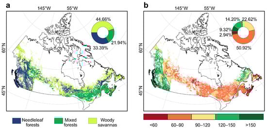
Figure 1.
Spatial patterns of undisturbed forest types and age categories in Canada. (a) Spatial distribution of undisturbed forests and relative proportions of forest types. (b) Spatial distribution of undisturbed forests by age categories and their relative proportions.
2.1.3. Forest Age
Forest age information was sourced from a global 1 km resolution dataset representing conditions around 2010 [41]. The dataset was created using machine learning models trained on more than 40,000 forest inventory plots, together with biomass and climate information, to provide spatially explicit estimates of forest age [41]. To ensure consistency with other datasets, the 1 km data were aggregated to a 0.05° resolution by calculating the mean forest age within each pixel. Forest ages were then categorized into five classes (<60, 60–90, 90–120, 120–150, and >150 years), as shown in Figure 1b.
2.1.4. Environmental Datasets
Monthly 2 m air temperature and surface solar radiation at 0.1° spatial resolution were retrieved from the ERA5-Land dataset [42] and resampled to 0.05° using bilinear interpolation. Annual values were then aggregated as follows: air temperature was calculated as the mean of monthly averages (T, °C), while surface solar radiation downwards (SSRD, J/m2) was computed as the sum of monthly totals.
Land surface temperature (LST) data were derived from the MODIS product for land surface temperature and emissivity (MOD11A1) [43], which provides daily estimates of LST at a spatial resolution of 1 km. After performing quality control on the Google Earth Engine (GEE) platform, we aggregated the daily retrievals to annual composites at a 0.05° resolution.
The Standardized Precipitation Evapotranspiration Index (SPEI) was derived from the Global SPEI database, which was generated based on the monthly precipitation and temperature data [44]. SPEI accounts for both precipitation and evaporation, making it a robust metric for drought characterization [45]. It constructs cumulative water deficit series over various timescales and standardizes them to obtain SPEI values, where higher values indicate wetter conditions and lower values represent drier conditions. In this study, we used the 12-month SPEI (SPEI-12) dataset at its native 0.5° resolution. The final monthly value of each year was employed as an annual drought proxy. This proxy dataset was then spatially resampled to a 0.05° resolution for subsequent integrated analyses.
The soil moisture (SM) data were obtained from the European Space Agency’s Climate Change Initiative (ESA CCI) soil moisture datasets [46,47]. This product provides a long-term, global record of surface soil moisture by combining retrievals from a series of active and passive microwave satellite sensors [48]. The active component merges data from scatterometers, while the passive component integrates observations from radiometers [49]. The combined product, which merges both active and passive retrievals, was used in this study to ensure a robust representation of soil moisture dynamics. The original data, provided at a daily temporal resolution and a spatial resolution of 0.25°, were resampled to 0.05° and aggregated to monthly mean values.
The Global Soil Dataset for Earth System Modeling (GSDE) provides data on various soil characteristics, including particle-size distribution, organic carbon content, and nutrient levels, with a spatial resolution of 5 arc-minutes (approximately 10 km) [50]. In this study, we used the soil organic carbon (SOC, %), and soil clay content of the surface layer (SC, %). These variables were resampled to a 0.05° resolution using bilinear interpolation to match the spatial scale of other datasets.
Digital elevation data (DEM) were obtained from the Copernicus DEM (COP-DEM) dataset, which is derived from Sentinel-1 and Sentinel-2 satellites observations, along with remote sensing radar and optical images under the framework of the Copernicus project [51]. The dataset covers the full global landmass of the time frame of data acquisition [52] and shows superior accuracy and reliability in areas with complex terrain conditions compared to other available elevation datasets [53,54]. The 0.05° DEM was generated by averaging the 30 m resolution data.
2.2. Methods
2.2.1. Vegetation Resilience
To remove seasonal and trend components from the original LAI data, we applied Seasonal-Trend decomposition with Loess (STL) [55] to the LAI time series at each pixel. This approach allows flexible separation of nonstationary seasonal signals and long-term trends, thereby isolating short-term fluctuations that are more appropriate for resilience assessment. The resulting residuals, which represent the detrended and de-seasonalized LAI were then used for AR(1) coefficient calculations.
AR(1) coefficients were calculated using a conditional least-squares method [56] within a sliding five-year window (60 months) (Equation (1)).
where is the residual component of the decomposed LAI time series, is the one-time-step-lagged series, AR(1) is the autoregressive coefficient, and is the residual term.
To evaluate the robustness of the detrending procedure, we tested multiple STL trend window sizes and assessed their influence on the resulting AR(1) estimates. The results from alternative STL decompositions (Figure A2) show highly consistent spatiotemporal patterns in AR(1) trends across different trend window settings, indicating that the detrending choice does not substantially affect the inferred resilience signals. In addition, sensitivity tests using different sliding window lengths for AR(1) estimation yielded comparable results (Figure A3).
2.2.2. Trends and Transitions in Forest Resilience
Kendall’s was employed to assess resilience trends [11]. It is a non-parametric rank correlation coefficient used to detect monotonic trends in time series data. A positive value for AR(1) indicates increasing autocorrelation, reflecting declining ecosystem resilience, while a negative value suggests increasing resilience.
In addition to spatially depicting resilience trends using pixel-scale values, we also evaluated the trends in the mean AR(1) time series across the entire study area. A positive value for the mean LAI indicates a greening trend, whereas a negative value indicates browning trend.
To detect abrupt transitions in resilience, we applied the Break For Additive Season and Trend (BFAST) algorithm to the AR(1) time series for each pixel [11,57]. We specified a single structural break to identify the transition year that divides the time series into two segments: Phase 1 (pre-transition years) and Phase 2 (post-transition years). We specified a single structural breakpoint because resilience dynamics during 2001–2018 are characterized by one dominant and statistically significant regime shift across vegetation types (Figure A4), while allowing multiple breakpoints would increase sensitivity to short-term noise in pixel-wise AR(1) series and potentially lead to spurious or unstable transition detection [58]. Kendall’s for each pixel was then calculated separately for each phase at every pixel to quantify the temporal trend of resilience within the two periods. We focused on pixels that have significant trends (p < 0.05) in both phases and categorized resilience trajectories into two transition types: D-I: a shift from declining to increasing resilience; and I-D: a shift from increasing to declining resilience.
To further quantify resilience shifts (), we calculated the difference in Kendall’s between the two phases:
where and are the Kendall’s values for Phases 1 and Phase 2, respectively. The signed values preserve the direction of transitions, while the absolute values indicate the magnitude of change. Specifically, a positive corresponds to a transition from increasing to decreasing resilience (I-D), whereas a negative corresponds to a transition from decreasing to increasing resilience (D-I). Larger absolute values reflect stronger resilience shifts.
2.2.3. XGBoost-SHAP Interpretation Framework
To investigate the drivers of resilience shifts (), we employed the Extreme gradient boosting (XGBoost) model. This ensemble learning approach constructs prediction models through an iterative decision tree framework [59] and was applied using eight environmental variables as predictors.
For the five temporally varying factors, which are 2 m air temperature (T), land surface temperature (LST), Standardized Precipitation Evapotranspiration Index (SPEI), soil moisture (SM), and surface solar downward radiation (SSRD), we calculated their change () the difference between their mean annual values in the post- and pre-transition phases for each pixel. Annual means were used to capture climatic effects across all seasons. The change for a given factor was computed as:
where and are the mean annual values of the factor over Phases 1 and Phase 2, respectively. These phases are defined individually for each pixel based on the BFAST-identified transition year. For instance, for a pixel with a transition year of 2010, represents the mean temperature from 2010 to 2018 minus the mean temperature from 2001 to 2010.
The full set of predictors included: two temperature-related variables ( and ), two moisture-related variables ( and ), and four additional variables (, digital elevation model (DEM), soil organic carbon (SOC), and soil clay content (SC)) (Table A1, Figure A5).
Model implementation for XGBoost involved a structured workflow of training, hyperparameter tuning, and validation. We first partitioned the data, using a random subset comprising 40% of the available samples (n = 26,456) for model training. The random split was conducted with a fixed random state of 42 to ensure reproducibility. Subsequently, we optimized the XGBoost hyperparameters through a Bayesian search strategy [60]. Upon completing this training and validation process, we applied the final optimized XGBoost model to predict for all available samples (n = 66,142) to generate a spatially complete assessment of resilience shifts.
To interpret the model results, we combined the XGBoost algorithm with the SHapley Additive exPlanations (SHAP) framework [61]. SHAP provides local interpretability by quantifying the marginal contribution of each input variable to individual predictions of . SHAP decomposes model predictions into additive contributions from each feature, allowing for a systematic evaluation of both the direction and strength of their effects.
For each sample with features, the explanation’s attribution values for each feature should sum up to the model’s output :
where is the prediction values for sample , is the expected value of the model output, and is the SHAP value for feature .
In addition to computing SHAP values for each feature in each sample, we assessed global feature importance using the mean absolute SHAP value:
where is the input variable, is the data sample, and is total the number of data samples.
The SHAP framework provided insights into the individual contributions of each environmental driver to . Negative SHAP values corresponded to decreased values, indicating enhanced ecosystem resilience, whereas positive SHAP values corresponded to increased and associated reductions in resilience. The influence of each driver on was quantified by the magnitude of its absolute SHAP value. To further characterize spatial patterns in resilience drivers, we determined the dominant driver within each 0.05° pixel by selecting the variable exhibiting the highest absolute SHAP value.
The robustness of the XGB-SHAP framework can be affected by spatial autocorrelation and sampling variability, as geographically proximate observations are not independent, potentially inflating performance estimates under conventional random sampling or cross-validation [62,63]. To mitigate this limitation, we employed a spatial block-bootstrapping validation, partitioning the study area into 1° × 1° blocks and generating 100 bootstrap iterations. For each iteration, SHAP values were generated and the corresponding global feature importance rankings were derived. The consistency of driver importance across iterations confirmed that the robustness of our results.
3. Results
3.1. Spatial and Temporal Patterns of Resilience in Canada’s Undisturbed Forests During 2001–2018
The spatiotemporal distribution of resilience across Canada’s undisturbed forests between 2001 and 2018 revealed that the majority of regions (62.79%) experienced increasing resilience, with the most pronounced increases observed in the eastern part of Boreal Shield, Montane Cordillera, Pacific Maritime, and the western region of Atlantic Maritime ecozones (Figure 2a). In contrast, regions having declining resilience (37.31%) were primarily concentrated in the western region of Boreal Shield ecozone (Figure 2a). Repeating the analysis with an annual step between five-year AR(1) windows produced highly consistent spatial patterns and resilience proportions (Figure A6), confirming that our conclusions are not an artifact of window overlap.
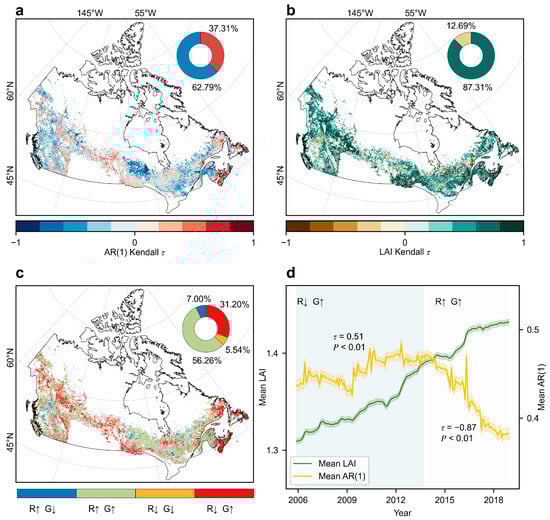
Figure 2.
Spatiotemporal patterns of resilience and greening dynamics in Canada’s undisturbed forests (2001–2018). (a) Spatial distribution of AR(1)-based resilience trends (Kendall’s ), with positive values indicating declining resilience and negative values indicating increasing resilience. (b) Spatial distribution of LAI trends (Kendall’s ), with positive values indicating greening and negative values indicating browning. (c) Spatial correspondence between resilience and greening trends (R: resilience, G: greening; ↑: increase, ↓: decline). (d) Temporal trajectories of mean resilience (yellow) and mean LAI (green). Shaded areas represent the 95% confidence interval for each factor, with the resilience interval magnified tenfold for visual purposes. Pixels with non-significant Kendall’s results (p > 0.05) are shown in gray to distinguish them from statistically significant trends in (a–c). The circular insets in (a,b) show the proportional distribution of resilience and greening trends, respectively (blue and green: increasing; red and brown: declining). To ensure comparability, LAI trends in (b) were calculated using Kendall’s after applying the same 5-year sliding window averaging used in the AR(1) analysis. Mean LAI and mean AR(1) values in (d) are plotted at the end of each sliding window.
Forest greenness, as indicated by LAI trends, did not correspond spatially with the observed patterns of resilience patterns. Specifically, 87.31% of undisturbed forests experienced an increasing LAI trend between 2001 and 2018, whereas only 12.69% showed a decrease (Figure 2b). Notably, 38.2% of undisturbed forest regions had contrasting trends between resilience and greenness, with the most dominant pattern being a decline in resilience despite an increase in greenness (31.20%, Figure 2c).
The temporal dynamics of AR(1), divided via the BFAST method, revealed two distinct phases in the resilience trajectory of undisturbed forests. During Phase 1 (2005–2013), resilience declined significantly, as indicated by an increasing AR(1) trend ( = 0.51, p < 0.01). In contrast, Phase 2 (2013–2018) showed a marked increase in resilience, reflected by a decreasing AR(1) trend ( = −0.87, p < 0.01) (Figure 2d). In comparison, forest greenness, represented by LAI, displayed a continuous upward trend throughout the entire period (2005–2018), as evidenced by a significant positive value ( = 0.96, p < 0.01) (Figure 2d).
3.2. Resilience Transitions in Canada’s Undisturbed Forests
The resilience trajectories of Canada’s undisturbed forests were distinguished into two distinct phases based on the BFAST algorithm (Figure 3). We found that nearly half of the undisturbed forests (49.77%) experienced a shift from declining to increasing resilience (D-I), primarily located in the eastern part of Boreal Shield and the western Atlantic Maritime ecozones (Figure 3c). In contrast, transitions from increasing to decreasing resilience (I-D) accounted for a smaller proportion (23.05%) and were mainly distributed in the Boreal Cordillera and the western portion of the Boreal Shield ecozones (Figure 3c). Regions with no discernible directional change in resilience trends during 2001–2018 (NC) comprised 27.18% of the undisturbed forest areas (Figure 3c).
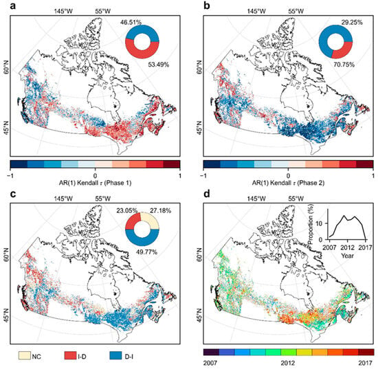
Figure 3.
Spatial patterns of resilience transitions and transition years in Canada’s undisturbed forests. (a) Spatial distribution of AR(1)-based resilience trends (Kendall’s ) during Phase 1 (pre-transition). (b) Same as (a) but for Phase 2 (post-transition). (c) Spatial distribution of resilience transition types. (d) Spatial distribution of resilience transition years and annual proportion of shifts. The circular insets in (a,b) show the proportional distribution of resilience trends (blue: increasing; red: declining). NC: no change in resilience trend between phases, exhibiting either persistent increase or decrease throughout the study period; I-D: increasing resilience in Phase 1 followed by declining resilience in Phase 2; D-I: declining resilience in Phase 1 followed by increasing resilience in Phase 2. For all panels (a–d), non-significant Kendall’s results (p > 0.05 in either phase) are indicated in gray to distinguish them from statistically significant trends.
Resilience transitions were predominantly concentrated in the years 2011 and 2014, where 14.87% and 14.25% of the study area, respectively, experienced shifts in resilience trajectories (Figure 3d). Spatially, resilience transitions in the central Boreal Shield tended to occur later (2013–2015) than other regions, where most transitions occurred earlier (2010–2012) (Figure 3d). Temporally, D-I transitions generally occurred later than I-D transitions, with the former concentrated in 2013–2015 and the latter in 2009–2012 (Figure A7).
A chi-square test [64] indicates that forest resilience transition types differ significantly among forest types and forest age classes (p < 0.01; Table A2 and Table A3). Across forest types, mixed forests had the highest proportion of resilience transitions (i.e., including I-D and D-I; 82.24%), followed by woody savannas (71.12%) and needleleaf forests (68.67%). Among these transitions, the shift from declining to increasing resilience (D-I) was the dominant pattern across all forest types and was particularly pronounced in mixed forests, where 74.39% of pixels exhibited a D-I transition (Figure 4a).
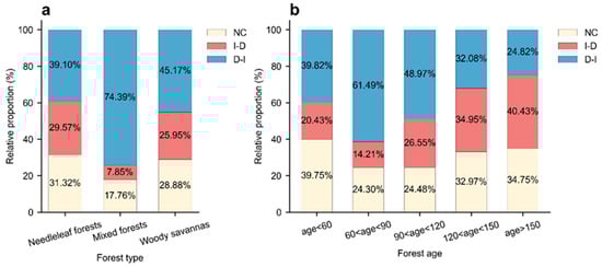
Figure 4.
Relative proportions of resilience transition types across various forest types and age classes. (a) Proportions of NC, I-D, and D-I transitions among different forest types. (b) Proportions of NC, I-D, and D-I transitions among different forest age classes.
Resilience transitions also varied across forest age classes. Forests younger than 60 years had the lowest proportion of resilience transition (60.25%) compared to older age groups (Figure 4b). By contrast, forests aged 60–90 years experienced the highest prevalence of transitions (75.70%), after which the proportion of transitions declined progressively with increasing age (Figure 4b). Moreover, the proportion of D-I transitions was highest in the 60–90-year age class (61.49%) and decreased with further increases in forest age (Figure 4b).
3.3. Response of Forest Resilience Transitions to Environmental Drivers
The magnitude of resilience shifts was quantified using the difference in Kendall’s () between the two phases before and after the transition point. Among regions where resilience shifted from declining to increasing (D-I), the largest absolute values were concentrated in the central Boreal Shield ecozone, whereas the greatest values for resilience shifted from increasing to declining (I-D) occurred in the Boreal Cordillera ecozone (Figure 5a). The distribution of transition types (i.e., D-I, and I-D) revealed pronounced asymmetry, with D-I transitions showing substantially greater magnitudes than I-D transitions (Figure 5b). Specifically, the mean for D-I transitions was −1.23, compared with 1.08 for I-D transition (Figure 5b), indicating a stronger intensity of resilience increase.
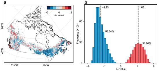
Figure 5.
Spatial patterns of the magnitude of resilience shifts () in Canada’s undisturbed forests. (a) Spatial distribution of values. (b) Histogram of pixel-scale . Pixels exhibiting no resilience shifts are shown in gray in (a). The gray dotted line and accompanying numbers in (b) indicate the mean values for D-I (−1.23) and I-D (1.08) transitions, respectively. The percentages (68.34% and 31.66%) in (b) represent the areal proportions of D-I (blue) and I-D (red) transitions, respectively.
We trained the XGBoost model to predict resilience shifts () using 40% of the available samples, achieving strong predictive skill on the test set (R2 > 0.71). Correlation and SHAP dependence analyses indicate limited multicollinearity among predictors, which does not materially affect the interpretation of and effects (Figure A8). Spatial block-bootstrap validation (100 iterations) further demonstrated model robustness, yielding a mean R2 of 0.41 ± 0.03 (standard deviation, SD) and a mean RMSE of 0.85 ± 0.02. The spatial distribution of pixel-level RMSE values showed a clear concentration at low error levels, with a median RMSE of approximately 0.55 (Figure A9), confirming the stability and robustness of model performance. Across the 100 spatial block-bootstrap iterations, SHAP analyses based on absolute SHAP values consistently ranked , DEM and as the dominant drivers of resilience shifts (Table A4). However, DEM showed high variability in importance across bootstrap samples, indicating its influence on resilience mainly reflects local effects in specific physiographic contexts rather than a uniform pattern across the study domain.
The spatial distribution of dominant drivers revealed that was the primary determinant of resilience shifts (), accounting for 38.79% of shifting regions. In the Eastern Boreal Shield, cooling corresponded to D-I transitions, while in the Boreal Cordillera, warming was associated with I-D transitions (Figure 5a, Figure 6a and Figure A5). Following , contributed 15.08% of the shifting regions, with its impact concentrated in the central Boreal Shield ecozone, where increases in moisture also coincided with D-I transitions (Figure 5a, Figure 6a and Figure A5). These two drivers ( and ) jointly accounted for 53.87% of the shifting regions (Figure 6a), underscoring the pivotal role of temperature and moisture in regulating undisturbed forest resilience shifts. DEM also emerged as an important driver, particularly in high-altitude areas of the Montane Cordillera ecozone (Figure 6a and Figure A5).
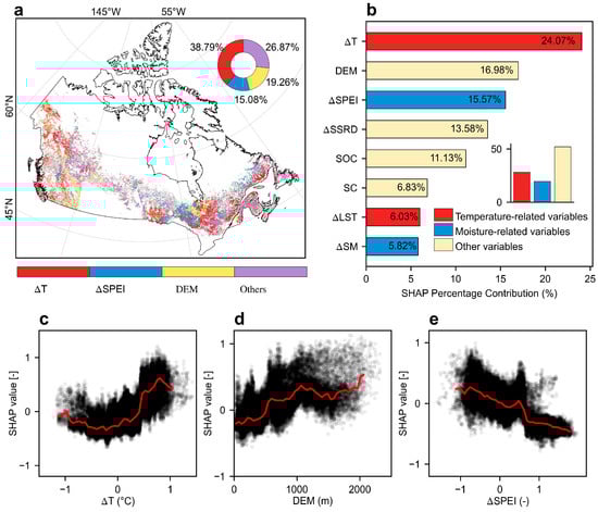
Figure 6.
Explanatory factors for resilience shifts () in Canada’s undisturbed forests. (a) Spatial distribution of dominant drivers associated with . (b) Relative importance of the drivers explaining the spatial variability of resilience shifts (). (c–e) Partial dependence plots of the top three drivers, namely, (c), DEM (d), (e). Pixels having no resilience shifts are shown in gray in (a). The bar chart in (b) shows the contribution proportions of three predictor categories: temperature-related variables ( and ), moisture-related variables ( and ), other variables (, DEM, SOC and SC). For panel (c–e), the y-axis represents the SHAP value for the corresponding predictor (x-axis), where positive values indicate increased and reduced resilience, while negative values indicate decreased and enhanced resilience. The red line indicates the median SHAP values across 50 bins of x-axis variables, plotted only for bins containing more than 50 samples.
The ranking of variable importance further emphasized the critical role of temperature-related variables (, and ), a which jointly explained 30.10% of the variance in (Figure 6b). Among them, was the dominant factor (24.07%) (Figure 6b), showing a positive correlation with SHAP values (Figure 6c). Since negative SHAP values denote resilience gains and positive values denote losses, the increase in SHAP values when exceeded 0 °C suggested that elevated temperatures substantially reduced forest resilience (Figure 6c). By comparison, had only a marginal contribution (6.03%, Figure 6b) and displayed little variation in SHAP values across its range (Figure A10). Following temperature, two moisture-related variables, and jointly explaining 21.39% of the variation in (Figure 6b). A negative correlation was observed between and SHAP values (Figure 6d), indicating that wetter conditions consistently enhance forest resilience.
In addition to temperature- and moisture-related variables, the four remaining variables (i.e., DEM, , SOC, and SC) collectively explained 48.52% of the variation in , with DEM contributing the most (16.98%, Figure 6b). Its positive correlation with SHAP values indicates reduced forest resilience at higher elevations (Figure 6e). The influences of , SOC, and SC were limited, contributing 13.58%, 11.13%, and 6.83%, respectively (Figure 6b). SHAP analysis suggested a slight decline in resilience under enhanced solar radiation, as indicated by rising SHAP values with higher (Figure A10). By contrast, SHAP values for SOC and SC fluctuated around zero with no clear trends, suggesting their negligible effects on resilience (Figure A10).
4. Discussion
Our study showed that 62.79% of undisturbed forest regions in Canada experienced increasing resilience between 2001 and 2018, a pattern consistent with previous findings of an increasing trend of resilience in boreal ecosystems during the period 2000–2020 [15]. 38.20% of undisturbed forest regions showed asynchronous trends between resilience and greenness, suggesting that increases in greenness do not reflect enhanced ecosystem resilience. This decoupling corroborates prior studies suggesting that greening may reflect short-term productivity gains, whereas declining resilience often arises from underlying structural stress or disturbance [11,15]. Consequently, transient increases in vegetation vigor can obscure deeper ecosystem vulnerability [65]. One explanation is that vegetation may prioritize carbon allocation to rapid canopy recovery following disturbances, while sacrificing investments in structural components such as root biomass or woody tissue that are critical for long-term stability [66,67]. Moreover, when stand density exceeds environmental thresholds, intensified resource competition can induce physiological stress and constrain growth, thereby diminishing resilience despite stable or increasing canopy greenness [68].
Resilience shifts across Canada’s undisturbed forests were predominantly characterized by D-I transitions (i.e., resilience shifts from declining to increasing trends). These transitions displayed distinct spatial patterns across forest types and age classes. Notably, mixed-species forests had the most pronounced resilience gains, which can be attributable to their higher functional diversity and structural complexity [69]. Functional diversity enhances forest resilience by broadening the range of species responses to disturbances and reducing the susceptibility of ecosystem functions to perturbations [70]. In mixed-species forests, complementary functional traits, such as variation in water-use strategies, photosynthetic capacities, rooting depths, and growth phenology, allow different species to exploit resources at different times or from different soil layers, reduce direct competition, and provide redundancy in critical ecosystem functions [71]. These mechanisms promote asynchronous species responses, buffer fluctuations in productivity and biomass, and stabilize carbon and nutrient cycling, thereby improving recovery and maintaining ecosystem functioning following disturbances [70,72,73]. Similarly, in woody savannas, the structural openness and coexistence of woody and herbaceous components create multiple functional niches. Trees and grasses differ in rooting depths, phenology, and water or nutrient uptake strategies, which facilitates resource partitioning and reduces competition [74]. The lower canopy density and interspersed herbaceous vegetation also buffer microclimatic conditions, moderate soil temperature and moisture variability, and allow more rapid adjustments of ecosystem processes to environmental fluctuations. Together, these mechanisms of functional complementarity, redundancy, and asynchrony enable woody savannas to achieve higher resilience gains compared with more structurally uniform coniferous forests. Moreover, forest age also showed influence on resilience shifts. The greatest resilience gains were found in intermediate-aged forests (60–90 years), likely reflecting optimal carbon allocation strategies. Young forests prioritize carbon investment in rapid structural growth, limiting the accumulation of nonstructural carbon reserves and defensive capacity, whereas old forests allocate more carbon to maintenance and long-term structural support, reducing physiological flexibility and post-disturbance recovery potential. Intermediate-aged forests strike a balance among growth, nonstructural carbon storage, and defense, maintaining productivity while storing sufficient carbon to buffer stress. These nonstructural carbon reserves provide readily available energy for metabolism, repair, and regrowth under environmental stress, enhancing the forest’s ability to resist disturbances and recover afterward [75,76]. This balance enhances the capacity of intermediate-aged forests to withstand and recover from environmental stress, resulting in comparatively higher resilience. These findings suggested that mixed-species and intermediate-aged forests may play a pivotal role in sustaining ecosystem stability under future environmental change.
We found that lower temperatures and higher moisture availability jointly enhanced resilience across Canada’s undisturbed forests. While previous studies have suggested that rising temperatures promote boreal forest growth by extending the growth season and enhancing photosynthetic activity [7,15], which are generally interpreted as increasing adaptive capacity and resilience [77,78,79], our results reveal a contrasting pattern. Specifically, we observed a negative effect of warming on forest resilience, consistent with recent findings that warming has not substantially enhanced forest growth in boreal regions [10,80,81,82]. Forest growth mainly reflects short-term productivity, whereas resilience represents long-term ecosystem stability and recovery capacity. Warming-induced growth stimulation in boreal forests is often limited or transient and can be offset by water stress and other climatic constraints. Long-term ecosystem studies further indicate that, even in regions showing short-term greening trends, sustained warming may reduce the growth of dominant boreal species and increase their vulnerability to disturbance [83], highlighting that temporary gains in productivity do not necessarily translate into long-term ecosystem stability. This discrepancy, in which resilience is higher under cooler conditions, can be attributed to the narrow thermal niches and limited tolerance to temperature variability characteristic of boreal region ecosystems [84]. In high-latitude regions, rising temperatures can push physiological processes beyond their thresholds, thereby constraining rather than promoting post-disturbance recovery [85]. Our results support the perspective that resilience in cold-region ecosystems is more likely to be maintained under cooler conditions [13,86,87]. In addition to the temperature effects, increased moisture availability can further enhance resilience by alleviating water stress and promoting post-disturbance recovery [25,88,89]. These findings underscore the necessity of integrating both temperature and water availability into forest management and conservation strategies, particularly under climate change scenarios, to safeguard the stability and adaptive capacity of boreal and high-latitude forest ecosystems.
Temporally, D-I resilience transitions were found to occur later (2013–2015) than the I-D transitions (2009–2012) during the 2001–2018 period (Figure A11). Between 2009 and 2012, elevated temperatures combined with declining SPEI values, indicative of intensified drought stress, coincided with a pronounced increase in I-D transitions, reflecting widespread losses of forest resilience (Figure A11). Notably, 2012 was an extreme drought year in northern North America [90], including parts of Canada [91]. In contrast, the subsequent period from 2013 to 2015, characterized by cooling temperatures and improved moisture conditions (as indicated by rising SPEI values), was associated with a notable rise in D-I transitions, indicating resilience gains (Figure A11). These findings emphasize the synergistic effects of rising temperatures and intensified drought, as elevated temperatures increase evapotranspiration, exacerbating water deficits and leading to more frequent periods of low water availability [92]. These combined stressors contribute to declining ecosystem resilience [93,94], whereas enhanced water availability under cooler climatic conditions promotes recovery.
Recent studies have suggested that residual noise and cloud contamination in LAI data can introduce biases in AR(1) estimates [32]. In this study, we adopted the GLASS 0.05° LAI dataset, which, employs Time Series Cloud Detection [95] and machine learning-based temporal reconstruction [96] to minimize such artifacts, thereby providing better temporal continuity and spatial completeness compared with other global products [35,97], and offering a more robust basis for long-term AR(1) calculations. Nevertheless, the relatively coarse spatial resolution (0.05°) may limit the detection of fine-scale resilience transitions, particularly in topographically complex or heterogeneous forest landscapes, and may obscure subtle disturbance processes such as low-intensity degradation, insect outbreaks, windthrow, or small fires. As our analysis focuses on undisturbed forests, such disturbances may remain undetected at this scale and threshold. In addition, uncertainties in ancillary datasets may propagate into the analysis, for example, the global 1 km forest age product contains notable uncertainties in boreal regions [41], which are beyond the primary scope of this study.
In recent years, Canada’s forests have experienced frequent wildfire disturbances [98], with numerous studies indicating that such events have substantially diminished forest resilience [16,99]. This decline in resilience has critically constrained forest carbon sequestration capacity across Canada during 2001–2018. The present study systematically assessed the resilience of undisturbed forests, revealing a notable upward trend in resilience across Canada, particularly under conditions characterized by cooler temperatures and adequate moisture availability. These findings suggest that despite the detrimental impacts of wildfire disturbances on forest ecosystems, the enhanced resilience observed in undisturbed forests may serve as a buffering and recovery mechanism, partially compensating for resilience losses induced by wildfires.
5. Conclusions
We analyzed resilience dynamics from 2001 to 2018 across Canada’s undisturbed forests using the AR(1) metric derived from remotely sensed LAI data and found a widespread increasing trend in resilience across most forested areas. This pattern occurred alongside a persistent greening trend, highlighting the partial decoupling between forest greening and ecosystem resilience. Pixel-scale analysis of resilience transitions revealed that 49.77% of areas underwent a shift from declining to increasing resilience (D-I), while 23.05% experienced the inverse transition (I-D). These transition patterns were closely associated with forest type and age, with mixed and intermediate-age forests showing a higher proportion of D-I transitions. Further analyses indicated that temperature and moisture availability are the primary climatic drivers of resilience shifts (), with cooler temperatures and sufficient moisture promoting enhanced forest resilience. These findings provide a spatially explicit layer of forest resilience and its key drivers, offering insights to inform targeted conservation and management under climate change.
Author Contributions
Conceptualization, T.C.; methodology, C.Y. and T.C.; validation, C.Y. and T.C.; formal analysis, C.Y. and T.C.; resources, C.Y. and T.C.; data curation, C.Y. and T.C.; writing—original draft preparation, C.Y.; writing—review and editing, C.Y., T.C., L.F., J.W. and J.-P.W.; visualization, C.Y.; supervision, T.C.; funding acquisition, T.C. All authors have read and agreed to the published version of the manuscript.
Funding
This work was supported by the National Natural Science Foundation of China (42201364), and the Opening Funds from Chongqing Jinfo Mountain Karst Ecosystem National Research and Observation Station (JFS2023A02).
Data Availability Statement
The original contributions presented in this study are included in the article. Further inquiries can be directed to the corresponding author.
Acknowledgments
The authors sincerely appreciate the Nanjing Forestry University for its support and assistance in this article, as well as all the teachers for their valuable suggestions during the research process.
Conflicts of Interest
The authors declare no conflicts of interest.
Appendix A

Table A1.
The predictive variables as inputs for the XGBoost machine learning models.
Table A1.
The predictive variables as inputs for the XGBoost machine learning models.
| Categories | Predictor Variables | Unit |
|---|---|---|
| Temperature-related variables | Changes in 2 m air temperature | °C |
| Changes in land surface temperature | °C | |
| Moisture-related variables | Changes in Standardized Precipitation Evapotranspiration Index | unitless |
| Changes in soil moisture | m3/m3 | |
| Other variables | Changes in annual total surface solar radiation downwards | J/m2 |
| Digital elevation (DEM) | m | |
| Soil organic carbon of the surface layer (SOC) | % | |
| Soil clay content of the surface layer (SC) | % |
Table A2.
Pixel counts of forest resilience transition types across forest types and results of the chi-square test.
Table A2.
Pixel counts of forest resilience transition types across forest types and results of the chi-square test.
| Forest Types | Number of Pixels by Transition Type | SUM | P | |||
|---|---|---|---|---|---|---|
| NC | I-D | D-I | ||||
| Needleleaf forests | 10,884 | 10,276 | 13,586 | 34,746 | 8089.18 | <0.01 |
| Mixed forests | 4199 | 1856 | 17,589 | 23,644 | ||
| Woody savannas | 13,255 | 11,908 | 20,727 | 45,890 | ||
| Sum | 28,338 | 24,040 | 51,902 | 104,280 | ||
Table A3.
Pixel counts of forest resilience transition types across forest age classes and results of the chi-square test.
Table A3.
Pixel counts of forest resilience transition types across forest age classes and results of the chi-square test.
| Forest Ages | Number of Pixels by Transition Type | SUM | P | |||
|---|---|---|---|---|---|---|
| NC | I-D | D-I | ||||
| Age < 60 | 1255 | 645 | 1257 | 3157 | 8576.87 | <0.01 |
| 60 < age < 90 | 12,163 | 7112 | 30,783 | 50,058 | ||
| 90 < age < 120 | 5982 | 6487 | 11,964 | 24,433 | ||
| 120 < age < 150 | 5848 | 6201 | 5691 | 17,740 | ||
| Age > 150 | 3090 | 3595 | 2207 | 8892 | ||
| Sum | 28,338 | 24,040 | 51,902 | 104,280 | ||
Table A4.
Stability of SHAP-based feature importance rankings evaluated using 100 spatial block-bootstrap iterations.
Table A4.
Stability of SHAP-based feature importance rankings evaluated using 100 spatial block-bootstrap iterations.
| Features | Mean |SHAP| | SD of |SHAP| | SD of Rank |
|---|---|---|---|
| 0.2381 | 0.0188 | 0.7125 | |
| DEM | 0.2031 | 0.0173 | 2.5662 |
| 0.1542 | 0.0092 | 0.0000 | |
| 0.1440 | 0.0092 | 0.7125 | |
| SOC | 0.1351 | 0.0083 | 1.0812 |
| SC | 0.0940 | 0.0060 | 1.6710 |
| 0.0669 | 0.0039 | 2.6176 | |
| 0.0598 | 0.0038 | 1.7871 |

Figure A1.
Map of the study area showing Canadian ecozones.
Figure A1.
Map of the study area showing Canadian ecozones.


Figure A2.
Tests of robustness for detrending the LAI time series. The LAI time series was detrended and de-seasonalised using seasonal–trend decomposition based on STL, with the seasonal component fixed as periodic. The robustness of AR(1) estimates was evaluated by varying the trend window length (t.window = 13, 19, 25, 49, 73 and 97 months). (a) Example of trends removed under different t.window choices for a representative pixel LAI time series (raw LAI time series shown in gray). (b) Mean AR(1) time series corresponding to each t.window choice, with AR(1) values plotted at the end of each 5-year (60-month) sliding window. (c–h) Histograms of pixel-level Kendall’s values across different t.window settings.


Figure A3.
Robustness of LAI AR(1) to sliding window length. (a) Mean AR(1) time series using sliding windows of 5 years (60 months), 7 years (84 months) and 10 years (120 months). AR(1) values are plotted at the middle of each corresponding window. (b–d) Histograms of pixel-level Kendall’s values for the three window lengths.


Figure A4.
Temporal trajectories of mean resilience across needleleaf forests (a), mixed forests (b) and woody savannas (c).
Figure A4.
Temporal trajectories of mean resilience across needleleaf forests (a), mixed forests (b) and woody savannas (c).


Figure A5.
Spatial distribution of environmental factors in Canada’s undisturbed forests. (a) Changes in 2 m air temperature changes (). (b) Changes in Standardized Precipitation Evapotranspiration Index (). (c) Digital elevation (DEM). (d) Changes in soil moisture (). (e) Changes in surface solar radiation downwards (). (f) The soil organic carbon (SOC). (g) Changes in the land surface temperature (). (h) The soil clay content (SC).


Figure A6.
Spatiotemporal patterns of resilience and greening dynamics in Canada’s undisturbed forests (2001–2018) using annually stepped five-year windows. (a) Temporal trajectories of mean resilience. (b) Spatial distribution of AR(1)-based resilience trends (Kendall’s ), with positive values indicating declining resilience and negative values indicating increasing resilience. Shaded areas represent the 95% confidence interval for each factor, with the resilience interval magnified tenfold for visual purposes. Pixels with non-significant Kendall’s τ results (p > 0.05) are shown in gray to distinguish them from statistically significant trends. The circular insets in (b) show the proportional distribution of resilience trends, (blue: increasing; red: declining).


Figure A7.
Spatial patterns of transition years. (a) I-D transitions. (b) D-I transitions.
Figure A7.
Spatial patterns of transition years. (a) I-D transitions. (b) D-I transitions.


Figure A8.
Pairwise Pearson correlation among predictor variables and SHAP dependence analysis for and . (a) Pearson correlation heatmap for the eight predictor variables. (b) SHAP dependence plots for and .
Figure A8.
Pairwise Pearson correlation among predictor variables and SHAP dependence analysis for and . (a) Pearson correlation heatmap for the eight predictor variables. (b) SHAP dependence plots for and .


Figure A9.
Robustness of XGBoost model performance assessed by spatial block bootstrapping cross-validation. (a) Spatial distribution of mean RMSE across 100 spatial block-bootstrap iterations. (b) Histogram of pixel-level RMSE values derived from the same bootstrap ensemble.
Figure A9.
Robustness of XGBoost model performance assessed by spatial block bootstrapping cross-validation. (a) Spatial distribution of mean RMSE across 100 spatial block-bootstrap iterations. (b) Histogram of pixel-level RMSE values derived from the same bootstrap ensemble.


Figure A10.
Partial dependence plots of various drivers. Partial dependence of (a) , (b) SOC, (c) (d) SC, (e) on resilience shifts (). The red line indicates the median SHAP values across 50 bins of x-axis variables, plotted only for bins containing more than 50 samples.
Figure A10.
Partial dependence plots of various drivers. Partial dependence of (a) , (b) SOC, (c) (d) SC, (e) on resilience shifts (). The red line indicates the median SHAP values across 50 bins of x-axis variables, plotted only for bins containing more than 50 samples.


Figure A11.
Interannual variations in climate drivers and resilience shift proportions. Shaded background highlights distinct climatic periods: purple denotes warmer, drier conditions (2009–2012), while yellow represents cooler, wetter conditions (2013–2015).
Figure A11.
Interannual variations in climate drivers and resilience shift proportions. Shaded background highlights distinct climatic periods: purple denotes warmer, drier conditions (2009–2012), while yellow represents cooler, wetter conditions (2013–2015).

References
- Pan, Y.; Birdsey, R.A.; Fang, J.; Houghton, R.; Kauppi, P.E.; Kurz, W.A.; Phillips, O.L.; Shvidenko, A.; Lewis, S.L.; Canadell, J.G. A large and persistent carbon sink in the world’s forests. Science 2011, 333, 988–993. [Google Scholar] [CrossRef]
- Kurz, W.A.; Shaw, C.; Boisvenue, C.; Stinson, G.; Metsaranta, J.; Leckie, D.; Dyk, A.; Smyth, C.; Neilson, E. Carbon in Canada’s boreal forest—A synthesis. Environ. Rev. 2013, 21, 260–292. [Google Scholar] [CrossRef]
- Brandt, J.P.; Flannigan, M.; Maynard, D.; Thompson, I.; Volney, W. An introduction to Canada’s boreal zone: Ecosystem processes, health, sustainability, and environmental issues. Environ. Rev. 2013, 21, 207–226. [Google Scholar] [CrossRef]
- Lee, H.; Calvin, K.; Dasgupta, D.; Krinner, G.; Mukherji, A.; Thorne, P.; Trisos, C.; Romero, J.; Aldunce, P.; Barret, K.; et al. IPCC, 2023: Climate Change 2023: Synthesis Report, Summary for Policymakers; Contribution of Working Groups I, II and III to the Sixth Assessment Report of the Intergovernmental Panel on Climate Change; Core Writing Team, Lee, H., Romero, J., Eds.; IPCC: Geneva, Switzerland, 2023. [Google Scholar]
- Gauthier, S.; Bernier, P.; Kuuluvainen, T.; Shvidenko, A.Z.; Schepaschenko, D.G. Boreal forest health and global change. Science 2015, 349, 819–822. [Google Scholar] [CrossRef] [PubMed]
- Post, E.; Alley, R.B.; Christensen, T.R.; Macias-Fauria, M.; Forbes, B.C.; Gooseff, M.N.; Iler, A.; Kerby, J.T.; Laidre, K.L.; Mann, M.E. The polar regions in a 2 C warmer world. Sci. Adv. 2019, 5, eaaw9883. [Google Scholar] [CrossRef]
- Wang, J.; Taylor, A.R.; D’Orangeville, L. Warming-induced tree growth may help offset increasing disturbance across the Canadian boreal forest. Proc. Natl. Acad. Sci. USA 2023, 120, e2212780120. [Google Scholar] [CrossRef]
- Piao, S.; Wang, X.; Park, T.; Chen, C.; Lian, X.; He, Y.; Bjerke, J.W.; Chen, A.; Ciais, P.; Tømmervik, H. Characteristics, drivers and feedbacks of global greening. Nat. Rev. Earth Environ. 2020, 1, 14–27. [Google Scholar] [CrossRef]
- Zampieri, M.; Grizzetti, B.; Meroni, M.; Scoccimarro, E.; Vrieling, A.; Naumann, G.; Toreti, A. Annual green water resources and vegetation resilience indicators: Definitions, mutual relationships, and future climate projections. Remote Sens. 2019, 11, 2708. [Google Scholar] [CrossRef]
- Girardin, M.P.; Bouriaud, O.; Hogg, E.H.; Kurz, W.; Zimmermann, N.E.; Metsaranta, J.M.; de Jong, R.; Frank, D.C.; Esper, J.; Büntgen, U. No growth stimulation of Canada’s boreal forest under half-century of combined warming and CO2 fertilization. Proc. Natl. Acad. Sci. USA 2016, 113, E8406–E8414. [Google Scholar] [CrossRef]
- Wang, Z.; Fu, B.; Wu, X.; Li, Y.; Feng, Y.; Wang, S.; Wei, F.; Zhang, L. Vegetation resilience does not increase consistently with greening in China’s Loess Plateau. Commun. Earth Environ. 2023, 4, 336. [Google Scholar] [CrossRef]
- Smith, T.; Traxl, D.; Boers, N. Empirical evidence for recent global shifts in vegetation resilience. Nat. Clim. Change 2022, 12, 477–484. [Google Scholar] [CrossRef]
- Yao, Y.; Liu, Y.; Fu, F.; Song, J.; Wang, Y.; Han, Y.; Wu, T.; Fu, B. Declined terrestrial ecosystem resilience. Glob. Change Biol. 2024, 30, e17291. [Google Scholar] [CrossRef]
- Guo, J.; Zhu, Z.; Gong, P. Global forest resilience change from 2001 to 2022. Int. J. Remote Sens. 2024, 45, 5889–5900. [Google Scholar] [CrossRef]
- Forzieri, G.; Dakos, V.; McDowell, N.G.; Ramdane, A.; Cescatti, A. Emerging signals of declining forest resilience under climate change. Nature 2022, 608, 534–539. [Google Scholar] [CrossRef] [PubMed]
- Whitman, E.; Parisien, M.-A.; Thompson, D.K.; Flannigan, M.D. Short-interval wildfire and drought overwhelm boreal forest resilience. Sci. Rep. 2019, 9, 18796. [Google Scholar] [CrossRef] [PubMed]
- Whitman, E.; Barber, Q.E.; Jain, P.; Parks, S.A.; Guindon, L.; Thompson, D.K.; Parisien, M.A. A modest increase in fire weather overcomes resistance to fire spread in recently burned boreal forests. Glob. Change Biol. 2024, 30, e17363. [Google Scholar] [CrossRef]
- Hart, S.J.; Henkelman, J.; McLoughlin, P.D.; Nielsen, S.E.; Truchon-Savard, A.; Johnstone, J.F. Examining forest resilience to changing fire frequency in a fire-prone region of boreal forest. Glob. Change Biol. 2019, 25, 869–884. [Google Scholar] [CrossRef]
- Bartels, S.F.; Chen, H.Y.; Wulder, M.A.; White, J.C. Trends in post-disturbance recovery rates of Canada’s forests following wildfire and harvest. For. Ecol. Manag. 2016, 361, 194–207. [Google Scholar] [CrossRef]
- Tyukavina, A.; Potapov, P.; Hansen, M.C.; Pickens, A.H.; Stehman, S.V.; Turubanova, S.; Parker, D.; Zalles, V.; Lima, A.; Kommareddy, I. Global trends of forest loss due to fire from 2001 to 2019. Front. Remote Sens. 2022, 3, 825190. [Google Scholar] [CrossRef]
- Watson, J.E.; Evans, T.; Venter, O.; Williams, B.; Tulloch, A.; Stewart, C.; Thompson, I.; Ray, J.C.; Murray, K.; Salazar, A. The exceptional value of intact forest ecosystems. Nat. Ecol. Evol. 2018, 2, 599–610. [Google Scholar] [CrossRef]
- Thompson, I.; Mackey, B.; McNulty, S.; Mosseler, A. Forest Resilience, Biodiversity, and Climate Change; Technical Series no. 43; Secretariat of the Convention on Biological Diversity: Montreal, QC, Canada, 2009; pp. 1–67.
- Wulder, M.A.; Hermosilla, T.; White, J.C.; Coops, N.C. Biomass status and dynamics over Canada’s forests: Disentangling disturbed area from associated aboveground biomass consequences. Environ. Res. Lett. 2020, 15, 094093. [Google Scholar] [CrossRef]
- Strickland, M.K.; Jenkins, M.A.; Ma, Z.; Murray, B.D. How has the concept of resilience been applied in research across forest regions? Front. Ecol. Environ. 2024, 22, e2703. [Google Scholar] [CrossRef]
- Boulton, C.A.; Lenton, T.M.; Boers, N. Pronounced loss of Amazon rainforest resilience since the early 2000s. Nat. Clim. Change 2022, 12, 271–278. [Google Scholar] [CrossRef]
- Yao, Z.; Van Velthoven, C.T.; Nguyen, T.N.; Goldy, J.; Sedeno-Cortes, A.E.; Baftizadeh, F.; Bertagnolli, D.; Casper, T.; Chiang, M.; Crichton, K. A taxonomy of transcriptomic cell types across the isocortex and hippocampal formation. Cell 2021, 184, 3222–3241. e3226. [Google Scholar] [CrossRef]
- Scheffer, M.; Bascompte, J.; Brock, W.A.; Brovkin, V.; Carpenter, S.R.; Dakos, V.; Held, H.; Van Nes, E.H.; Rietkerk, M.; Sugihara, G. Early-warning signals for critical transitions. Nature 2009, 461, 53–59. [Google Scholar] [CrossRef] [PubMed]
- Lenton, T.M.; Held, H.; Kriegler, E.; Hall, J.W.; Lucht, W.; Rahmstorf, S.; Schellnhuber, H.J. Tipping elements in the Earth’s climate system. Proc. Natl. Acad. Sci. USA 2008, 105, 1786–1793. [Google Scholar] [CrossRef] [PubMed]
- Verbesselt, J.; Umlauf, N.; Hirota, M.; Holmgren, M.; Van Nes, E.H.; Herold, M.; Zeileis, A.; Scheffer, M. Remotely sensed resilience of tropical forests. Nat. Clim. Change 2016, 6, 1028–1031. [Google Scholar] [CrossRef]
- Scheffer, M.; Carpenter, S.R.; Lenton, T.M.; Bascompte, J.; Brock, W.; Dakos, V.; Van de Koppel, J.; Van de Leemput, I.A.; Levin, S.A.; Van Nes, E.H. Anticipating critical transitions. Science 2012, 338, 344–348. [Google Scholar] [CrossRef]
- Wu, J.; Sun, Z.; Yao, Y.; Liu, Y. Trends of Grassland Resilience under Climate Change and Human Activities on the Mongolian Plateau. Remote Sens. 2023, 15, 2984. [Google Scholar] [CrossRef]
- Cai, M.; Zhang, Y.; Qiu, J. Estimating Ecosystem Resilience from Noisy Observational Data. Glob. Change Biol. 2025, 31, e70370. [Google Scholar] [CrossRef]
- Bathiany, S.; Bastiaansen, R.; Bastos, A.; Blaschke, L.; Lever, J.; Loriani, S.; De Keersmaecker, W.; Dorigo, W.; Milenković, M.; Senf, C. Ecosystem resilience monitoring and early warning using earth observation data: Challenges and outlook. Surv. Geophys. 2025, 46, 265–301. [Google Scholar] [CrossRef]
- Xiao, Z.; Liang, S.; Wang, J.; Xiang, Y.; Zhao, X.; Song, J. Long-time-series global land surface satellite leaf area index product derived from MODIS and AVHRR surface reflectance. IEEE Trans. Geosci. Remote Sens. 2016, 54, 5301–5318. [Google Scholar] [CrossRef]
- Xiao, Z.; Liang, S.; Wang, J.; Chen, P.; Yin, X.; Zhang, L.; Song, J. Use of general regression neural networks for generating the GLASS leaf area index product from time-series MODIS surface reflectance. IEEE Trans. Geosci. Remote Sens. 2013, 52, 209–223. [Google Scholar] [CrossRef]
- Friedl, M.; Sulla-Menashe, D. MODIS/Terra+ Aqua land cover type yearly L3 Global 0.05 Deg CMG V061. In NASA EOSDIS Land Processes Distributed Active Archive Center (DAAC) Data Set; NASA Land Processes Distributed Active Archive Center: Sioux Falls, SD, USA, 2022. [Google Scholar] [CrossRef]
- Hansen, M.C.; Potapov, P.V.; Moore, R.; Hancher, M.; Turubanova, S.A.; Tyukavina, A.; Thau, D.; Stehman, S.V.; Goetz, S.J.; Loveland, T.R. High-resolution global maps of 21st-century forest cover change. Science 2013, 342, 850–853. [Google Scholar] [CrossRef] [PubMed]
- Giglio, L.; Justice, C.; Boschetti, L.; Roy, D. MODIS/terra+ aqua burned area monthly L3 global 500m SIN grid V061. In NASA EOSDIS Land Processes Distributed Active Archive Center (DAAC) Data Set; NASA Land Processes Distributed Active Archive Center: Sioux Falls, SD, USA, 2021. [Google Scholar] [CrossRef]
- Fan, L.; Wigneron, J.-P.; Ciais, P.; Chave, J.; Brandt, M.; Sitch, S.; Yue, C.; Bastos, A.; Li, X.; Qin, Y. Siberian carbon sink reduced by forest disturbances. Nat. Geosci. 2023, 16, 56–62. [Google Scholar] [CrossRef]
- Wiken, E.; Gauthier, D.; Marshall, I.; Lawton, K.; Hirvonen, H. Canadian Council on Ecological Areas: A perspective on Canada’s Ecosystems; Canadian Council on Ecological Areas: Ottawa, ON, Canada, 1996. [Google Scholar]
- Besnard, S.; Koirala, S.; Santoro, M.; Weber, U.; Nelson, J.; Gütter, J.; Herault, B.; Kassi, J.; N’Guessan, A.; Neigh, C. Mapping global forest age from forest inventories, biomass and climate data. Earth Syst. Sci. Data Discuss. 2021, 13, 4881–4896. [Google Scholar] [CrossRef]
- Muñoz-Sabater, J.; Dutra, E.; Agustí-Panareda, A.; Albergel, C.; Arduini, G.; Balsamo, G.; Boussetta, S.; Choulga, M.; Harrigan, S.; Hersbach, H. ERA5-Land: A state-of-the-art global reanalysis dataset for land applications. Earth Syst. Sci. Data 2021, 13, 4349–4383. [Google Scholar] [CrossRef]
- Wan, Z.; Hook, S.; Hulley, G. MYD11A1 MODIS/aqua land surface temperature/emissivity daily L3 global 1km SIN grid V006. In NASA EOSDIS Land Processes Distributed Active Archive Center (DAAC) Data Set; NASA Land Processes Distributed Active Archive Center: Sioux Falls, SD, USA, 2015. [Google Scholar] [CrossRef]
- Beguería, S.; Serrano, S.M.V.; Reig-Gracia, F.; Garcés, B.L. SPEIbase v.2.10 [Dataset]: A Comprehensive Tool for Global Drought Analysis. 2024. Available online: https://digital.csic.es/handle/10261/364137 (accessed on 6 August 2025).
- Vicente-Serrano, S.M.; Beguería, S.; López-Moreno, J.I. A multiscalar drought index sensitive to global warming: The standardized precipitation evapotranspiration index. J. Clim. 2010, 23, 1696–1718. [Google Scholar] [CrossRef]
- Dorigo, W.; Preimesberger, W.; Moesinger, L.; Pasik, A.; Scanlon, T.; Hahn, S. ESA Soil Moisture Climate Change Initiative (Soil_Moisture_cci): COMBINED product, Version 09.1. NERC EDS Centre for Environmental Data Analysis. 15 October 2024. Available online: https://catalogue.ceda.ac.uk/uuid/0e346e1e1e164ac99c60098848537a29/ (accessed on 6 October 2025).
- Gruber, A.; Scanlon, T.; Van Der Schalie, R.; Wagner, W.; Dorigo, W. Evolution of the ESA CCI Soil Moisture climate data records and their underlying merging methodology. Earth Syst. Sci. Data 2019, 11, 717–739. [Google Scholar] [CrossRef]
- Dorigo, W.; Wagner, W.; Albergel, C.; Albrecht, F.; Balsamo, G.; Brocca, L.; Chung, D.; Ertl, M.; Forkel, M.; Gruber, A. ESA CCI Soil Moisture for improved Earth system understanding: State-of-the art and future directions. Remote Sens. Environ. 2017, 203, 185–215. [Google Scholar] [CrossRef]
- Liu, Y.; Dorigo, W.A.; Parinussa, R.; de Jeu, R.A.; Wagner, W.; McCabe, M.F.; Evans, J.; Van Dijk, A. Trend-preserving blending of passive and active microwave soil moisture retrievals. Remote Sens. Environ. 2012, 123, 280–297. [Google Scholar] [CrossRef]
- Wei, S.; Dai, Y.; Duan, Q.; Liu, B.; Yuan, H. A global soil data set for earth system modeling. J. Adv. Model. Earth Syst. 2014, 6, 249–263. [Google Scholar] [CrossRef]
- Agency, E.S. Copernicus Global Digital Elevation Model. 2024. Available online: https://portal.opentopography.org/datasetMetadata?otCollectionID=OT.032021.4326.1 (accessed on 6 August 2025).
- Airbus, Z. Copernicus DEM: Copernicus Digital Elevation Model Product Handbook; Airbus Leiden: Leiden, The Netherlands, 2020. [Google Scholar]
- Guth, P.L.; Geoffroy, T.M. LiDAR point cloud and ICESat-2 evaluation of 1 second global digital elevation models: Copernicus wins. Trans. GIS 2021, 25, 2245–2261. [Google Scholar] [CrossRef]
- Trevisani, S.; Skrypitsyna, T.; Florinsky, I. Global digital elevation models for terrain morphology analysis in mountain environments: Insights on Copernicus GLO-30 and ALOS AW3D30 for a large Alpine area. Environ. Earth Sci. 2023, 82, 198. [Google Scholar] [CrossRef]
- Cleveland, R.B.; Cleveland, W.S.; McRae, J.E.; Terpenning, I. STL: A seasonal-trend decomposition. J. Off. Stat 1990, 6, 3–73. [Google Scholar]
- Dakos, V.; Carpenter, S.R.; Brock, W.A.; Ellison, A.M.; Guttal, V.; Ives, A.R.; Kéfi, S.; Livina, V.; Seekell, D.A.; van Nes, E.H. Methods for detecting early warnings of critical transitions in time series illustrated using simulated ecological data. PLoS ONE 2012, 7, e41010. [Google Scholar] [CrossRef]
- Verbesselt, J.; Hyndman, R.; Newnham, G.; Culvenor, D. Detecting trend and seasonal changes in satellite image time series. Remote Sens. Environ. 2010, 114, 106–115. [Google Scholar] [CrossRef]
- Awty-Carroll, K.; Bunting, P.; Hardy, A.; Bell, G. An evaluation and comparison of four dense time series change detection methods using simulated data. Remote Sens. 2019, 11, 2779. [Google Scholar] [CrossRef]
- Chen, T.; Guestrin, C. Xgboost: A scalable tree boosting system. In Proceedings of the 22nd ACM SIGKDD International Conference on Knowledge Discovery and Data Mining 2016, San Francisco, CA, USA, 13–17 August 2016; pp. 785–794. [Google Scholar] [CrossRef]
- Wang, Y.; Ni, X.S. A XGBoost risk model via feature selection and Bayesian hyper-parameter optimization. arXiv 2019, arXiv:1901.08433. [Google Scholar] [CrossRef]
- Lundberg, S.M.; Erion, G.; Chen, H.; DeGrave, A.; Prutkin, J.M.; Nair, B.; Katz, R.; Himmelfarb, J.; Bansal, N.; Lee, S.-I. From local explanations to global understanding with explainable AI for trees. Nat. Mach. Intell. 2020, 2, 56–67. [Google Scholar] [CrossRef]
- Meyer, H.; Reudenbach, C.; Wöllauer, S.; Nauss, T. Importance of spatial predictor variable selection in machine learning applications–Moving from data reproduction to spatial prediction. Ecol. Model. 2019, 411, 108815. [Google Scholar] [CrossRef]
- Roberts, D.R.; Bahn, V.; Ciuti, S.; Boyce, M.S.; Elith, J.; Guillera-Arroita, G.; Hauenstein, S.; Lahoz-Monfort, J.J.; Schröder, B.; Thuiller, W. Cross-validation strategies for data with temporal, spatial, hierarchical, or phylogenetic structure. Ecography 2017, 40, 913–929. [Google Scholar] [CrossRef]
- McHugh, M.L. The chi-square test of independence. Biochem. Med. 2013, 23, 143–149. [Google Scholar] [CrossRef]
- Zhang, J.; Hao, X.; Liu, Y.; Li, X.; Liang, Q.; Sun, F.; Ci, M.; Li, Y. Vegetation greening does not significantly enhance ecosystem resilience in the Northern Hemisphere. Ecol. Indic. 2025, 177, 113762. [Google Scholar] [CrossRef]
- Poorter, H.; Niklas, K.J.; Reich, P.B.; Oleksyn, J.; Poot, P.; Mommer, L. Biomass allocation to leaves, stems and roots: Meta-analyses of interspecific variation and environmental control. New Phytol. 2012, 193, 30–50. [Google Scholar] [CrossRef]
- McDowell, N.G.; Allen, C.D.; Anderson-Teixeira, K.; Aukema, B.H.; Bond-Lamberty, B.; Chini, L.; Clark, J.S.; Dietze, M.; Grossiord, C.; Hanbury-Brown, A. Pervasive shifts in forest dynamics in a changing world. Science 2020, 368, eaaz9463. [Google Scholar] [CrossRef] [PubMed]
- Cui, J.; Lian, X.; Huntingford, C.; Gimeno, L.; Wang, T.; Ding, J.; He, M.; Xu, H.; Chen, A.; Gentine, P. Global water availability boosted by vegetation-driven changes in atmospheric moisture transport. Nat. Geosci. 2022, 15, 982–988. [Google Scholar] [CrossRef]
- Wright, A.; Schnitzer, S.A.; Reich, P.B. Living close to your neighbors: The importance of both competition and facilitation in plant communities. Ecology 2014, 95, 2213–2223. [Google Scholar] [CrossRef] [PubMed]
- Pardos, M.; Del Río, M.; Pretzsch, H.; Jactel, H.; Bielak, K.; Bravo, F.; Brazaitis, G.; Defossez, E.; Engel, M.; Godvod, K. The greater resilience of mixed forests to drought mainly depends on their composition: Analysis along a climate gradient across Europe. For. Ecol. Manag. 2021, 481, 118687. [Google Scholar] [CrossRef]
- Loreau, M.; Hector, A. Partitioning selection and complementarity in biodiversity experiments. Nature 2001, 412, 72–76. [Google Scholar] [CrossRef] [PubMed]
- Schnabel, F.; Liu, X.; Kunz, M.; Barry, K.E.; Bongers, F.J.; Bruelheide, H.; Fichtner, A.; Härdtle, W.; Li, S.; Pfaff, C.-T. Species richness stabilizes productivity via asynchrony and drought-tolerance diversity in a large-scale tree biodiversity experiment. Sci. Adv. 2021, 7, eabk1643. [Google Scholar] [CrossRef]
- Hisano, M.; Ghazoul, J.; Chen, X.; Chen, H.Y. Functional diversity enhances dryland forest productivity under long-term climate change. Sci. Adv. 2024, 10, eadn4152. [Google Scholar] [CrossRef]
- Case, M.F.; Nippert, J.B.; Holdo, R.M.; Staver, A.C. Root-niche separation between savanna trees and grasses is greater on sandier soils. J. Ecol. 2020, 108, 2298–2308. [Google Scholar] [CrossRef]
- Vangi, E.; Dalmonech, D.; Cioccolo, E.; Marano, G.; Bianchini, L.; Puchi, P.F.; Grieco, E.; Cescatti, A.; Colantoni, A.; Chirici, G. Stand age diversity (and more than climate change) affects forests’ resilience and stability, although unevenly. J. Environ. Manag. 2024, 366, 121822. [Google Scholar] [CrossRef] [PubMed]
- Vangi, E.; Dalmonech, D.; Cioccolo, E.; Marano, G.; Bianchini, L.; Puchi, P.F.; Grieco, E.; Cescatti, A.; Colantoni, A.; Chirici, G. Stand age diversity and climate change affect forests’ resilience and stability, although unevenly. bioRxiv 2023. [Google Scholar] [CrossRef]
- Dakos, V.; Matthews, B.; Hendry, A.P.; Levine, J.; Loeuille, N.; Norberg, J.; Nosil, P.; Scheffer, M.; De Meester, L. Ecosystem tipping points in an evolving world. Nat. Ecol. Evol. 2019, 3, 355–362. [Google Scholar] [CrossRef]
- Chaparro-Pedraza, P.C. Fast environmental change and eco-evolutionary feedbacks can drive regime shifts in ecosystems before tipping points are crossed. Proc. R. Soc. B 2021, 288, 20211192. [Google Scholar] [CrossRef]
- Runge, K.; Tucker, M.; Crowther, T.W.; Fournier de Laurière, C.; Guirado, E.; Bialic-Murphy, L.; Berdugo, M. Monitoring terrestrial ecosystem resilience using earth observation data: Identifying consensus and limitations across metrics. Glob. Change Biol. 2025, 31, e70115. [Google Scholar] [CrossRef]
- Girardin, M.P.; Hogg, E.H.; Bernier, P.Y.; Kurz, W.A.; Guo, X.J.; Cyr, G. Negative impacts of high temperatures on growth of black spruce forests intensify with the anticipated climate warming. Glob. Change Biol. 2016, 22, 627–643. [Google Scholar] [CrossRef]
- Gedalof, Z.e.; Berg, A.A. Tree ring evidence for limited direct CO2 fertilization of forests over the 20th century. Glob. Biogeochem. Cycles 2010, 24, GB3027. [Google Scholar] [CrossRef]
- Giguère-Croteau, C.; Boucher, É.; Bergeron, Y.; Girardin, M.P.; Drobyshev, I.; Silva, L.C.; Hélie, J.-F.; Garneau, M. North America’s oldest boreal trees are more efficient water users due to increased [CO2], but do not grow faster. Proc. Natl. Acad. Sci. USA 2019, 116, 2749–2754. [Google Scholar] [CrossRef]
- Berner, L.T.; Goetz, S.J. Satellite observations document trends consistent with a boreal forest biome shift. Glob. Change Biol. 2022, 28, 3275–3292. [Google Scholar] [CrossRef]
- Lancaster, L.T. On the macroecological significance of eco-evolutionary dynamics: The range shift–niche breadth hypothesis. Philos. Trans. R. Soc. B 2022, 377, 20210013. [Google Scholar] [CrossRef]
- D’Orangeville, L.; Houle, D.; Duchesne, L.; Phillips, R.P.; Bergeron, Y.; Kneeshaw, D. Beneficial effects of climate warming on boreal tree growth may be transitory. Nat. Commun. 2018, 9, 3213. [Google Scholar] [CrossRef]
- Reich, P.B.; Bermudez, R.; Montgomery, R.A.; Rich, R.L.; Rice, K.E.; Hobbie, S.E.; Stefanski, A. Even modest climate change may lead to major transitions in boreal forests. Nature 2022, 608, 540–545. [Google Scholar] [CrossRef] [PubMed]
- Xu, C.; Liu, H.; Anenkhonov, O.A.; Korolyuk, A.Y.; Sandanov, D.V.; Balsanova, L.D.; Naidanov, B.B.; Wu, X. Long-term forest resilience to climate change indicated by mortality, regeneration, and growth in semiarid southern Siberia. Glob. Change Biol. 2017, 23, 2370–2382. [Google Scholar] [CrossRef] [PubMed]
- Feng, Y.; Su, H.; Tang, Z.; Wang, S.; Zhao, X.; Zhang, H.; Ji, C.; Zhu, J.; Xie, P.; Fang, J. Reduced resilience of terrestrial ecosystems locally is not reflected on a global scale. Commun. Earth Environ. 2021, 2, 88. [Google Scholar] [CrossRef]
- Smith, T.; Boers, N. Global vegetation resilience linked to water availability and variability. Nat. Commun. 2023, 14, 498. [Google Scholar] [CrossRef]
- Mallya, G.; Zhao, L.; Song, X.; Niyogi, D.; Govindaraju, R. 2012 Midwest drought in the United States. J. Hydrol. Eng. 2013, 18, 737–745. [Google Scholar] [CrossRef]
- Najafi, E.; Khanbilvardi, R. Clustering and trend analysis of global extreme droughts from 1900 to 2014. arXiv 2018, arXiv:1901.00052. [Google Scholar] [CrossRef]
- Zhuang, Y.; Fu, R.; Lisonbee, J.; Sheffield, A.M.; Parker, B.A.; Deheza, G. Anthropogenic warming has ushered in an era of temperature-dominated droughts in the western United States. Sci. Adv. 2024, 10, eadn9389. [Google Scholar] [CrossRef]
- Jing, M.; Zhu, L.; Liu, S.; Cao, Y.; Zhu, Y.; Yan, W. Warming-induced drought leads to tree growth decline in subtropics: Evidence from tree rings in central China. Front. Plant Sci. 2022, 13, 964400. [Google Scholar] [CrossRef] [PubMed]
- Díaz-Martínez, P.; Ruiz-Benito, P.; Madrigal-González, J.; Gazol, A.; Andivia, E. Positive effects of warming do not compensate growth reduction due to increased aridity in Mediterranean mixed forests. Ecosphere 2023, 14, e4380. [Google Scholar] [CrossRef]
- Tang, H.; Yu, K.; Hagolle, O.; Jiang, K.; Geng, X.; Zhao, Y. A cloud detection method based on a time series of MODIS surface reflectance images. Int. J. Digit. Earth 2013, 6, 157–171. [Google Scholar] [CrossRef]
- Ma, H.; Liang, S. Development of the GLASS 250-m leaf area index product (version 6) from MODIS data using the bidirectional LSTM deep learning model. Remote Sens. Environ. 2022, 273, 112985. [Google Scholar] [CrossRef]
- Zheng, J.; Wang, M.; Liang, M.; Gao, Y.; Tan, M.L.; Liu, M.; Wang, X. Influence of Terrain on MODIS and GLASS Leaf Area Index (LAI) Products in Qinling Mountains Forests. Forests 2024, 15, 1871. [Google Scholar] [CrossRef]
- Wang, W.; Wang, X.; Flannigan, M.D.; Guindon, L.; Swystun, T.; Castellanos-Acuna, D.; Wu, W.; Wang, G. Canadian forests are more conducive to high-severity fires in recent decades. Science 2025, 387, 91–97. [Google Scholar] [CrossRef]
- Liu, Q.; Peng, C.; Schneider, R.; Cyr, D.; McDowell, N.G.; Kneeshaw, D. Drought-induced increase in tree mortality and corresponding decrease in the carbon sink capacity of Canada’s boreal forests from 1970 to 2020. Glob. Change Biol. 2023, 29, 2274–2285. [Google Scholar] [CrossRef]


Disclaimer/Publisher’s Note: The statements, opinions and data contained in all publications are solely those of the individual author(s) and contributor(s) and not of MDPI and/or the editor(s). MDPI and/or the editor(s) disclaim responsibility for any injury to people or property resulting from any ideas, methods, instructions or products referred to in the content. |
© 2026 by the authors. Licensee MDPI, Basel, Switzerland. This article is an open access article distributed under the terms and conditions of the Creative Commons Attribution (CC BY) license.