Nonuniformity Correction Algorithm for Infrared Image Sequences Based on Spatiotemporal Total Variation Regularization

Highlights

What are the main findings?

• The study proposes a novel denoising model incorporating a time-domain difference operator to effectively address nonuniform fixed-pattern noise in infrared image sequences.
• The algorithm successfully separates noise from observed images by leveraging the sparsity of noisy images in the time domain while using regularization-based priors to preserve details and reduce ghosting artifacts in high-resolution infrared remote sensing videos.

What are the implications of the main finding?

• The method provides a practical solution for eliminating complex fixed-pattern noise in real-world infrared imaging systems, particularly in dynamic environments where noise characteristics change over time.
• It demonstrates the potential for enhancing the quality of infrared remote sensing data from in-orbit cameras, enabling sharper image details and reduced artifacts, which could improve applications in environmental monitoring or astronomical observations.

Abstract

In infrared detectors, the readout circuits usually cause horizontal or vertical streak noise, whereas the infrared focal plane arrays experience triangular nonuniform fixed-pattern noise. In addition, imaging devices suffer from optically relevant fixed-pattern noise owing to the temperature. When the infrared camera is in orbit, it is affected by the photon effect, temperature change, and time drift. This makes the nonuniformity correction coefficients pertaining to the ground no longer applicable, resulting in the degradation of the nonuniformity correction effect. The existing methods are not fully applicable to triangular fixed-pattern noise or the fixed-pattern noise caused by detector optics. To address this situation, this paper proposes a nonuniformity correction method, namely infrared image sequences based on the optimization of $L_{2,1}$ group sparsity in the spatiotemporal domain. We established a nonuniformity correction model of differential operators in the spatiotemporal domain for infrared image sequences by applying the time-domain differential operator constraints to the images to denoise the image. This enables the adaptive correction of the nonuniformity of the above types of noise. We demonstrate that the proposed method is effective for triangular nonuniform and optically induced fixed-pattern noises. The proposed method was extensively evaluated using publicly available datasets and datasets containing image sequences of different scenes captured by a high-resolution infrared camera of the Qilu-2 satellite. The method has high robustness and good processing results with effective ghost suppression and significant reduction of nonuniform noise.

1. Introduction

Space-based infrared systems are being extensively researched and applied to agriculture, transportation, and military fields because of their all-day use, high concealment, and reproduction of the target’s radiation properties. However, during in-orbit operation, the detector is affected by the space environment, photon effect, temperature change, time drift, and other factors [1]. The nonuniformity correction coefficients measured on the ground are no longer applicable, and noise is an unavoidable factor in the remotely sensed image data, which not only impairs the visual quality of the remotely sensed images but also reduces their accuracy in subsequent target detection, tracking, identification, and other applications. To solve this problem, denoising algorithms are required to remove nonuniform noise from the images to compensate for the defects caused by noise on the signal-to-noise ratio and instrumentation.

Three types of nonuniform noise are commonly observed. The first is streak noise in Figure 1a, which is a special type of noise caused by the inconsistent response of each column or row of amplifiers in the current detector arrays or by the arrangement of readout circuits of the current detector arrays into rows or columns [2,3]. It results in different detector pixels outputting different grayscale values for the irradiance of the same object, such that each column or row of the image has a different bias for the image, resulting in horizontal or vertical striped nonuniform noise.

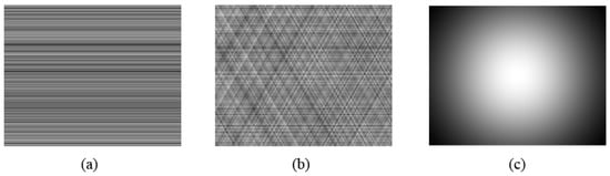
Figure 1. Three types of nonuniform noise. (a) Noise with bias nonuniformity. (b) Triangular fixed-pattern noise. (c) Optically induced fixed-pattern noise.

The second type of nonuniform noise is triangular fixed-pattern noise in Figure 1b [4,5], which can be disassembled into tilted stripe noise in multiple directions. Triangular fixed-pattern noise arises due to time drift, interference from the thermal noise of the analog-to-digital converter, and the resulting performance instability of each device in the detector array [6,7,8,9]. It is similar to the tilted nonuniform noise formed by horizontal or vertical streaks after geometric correction [10,11]. Most of the mainstream nonuniform correction methods are for single-direction, fixed-angle streak noise, and these methods applied to such noise can only remove single-direction streak noise, while nonuniform noise in other directions cannot be removed, and thus, these methods are not fully applicable to triangular fixed-pattern noise.

The third type is fixed-pattern noise caused by detector optics in Figure 1c. This is mainly due to the uneven responses of individual detectors, temperature fluctuations of the optical lenses, and other mechanical components [12,13], and it exhibits a slow drift with time and temperature. Smooth nonuniform noise will appear in the image, mainly gradual spatial inhomogeneity; that is, there is a significant difference in brightness between the center and the edges, which is manifested as obvious low-frequency spatial noise, which is reflected in the image as a bright and large spot, and the algorithms for removing streak noise are not very good at removing this kind of noise either. These three types of noise are the most common nonuniform noises and change with the detection environment. These noises seriously affect the image quality, and their removal requires the use of algorithms.

Nonuniformity correction methods can be broadly categorized into two groups: source- and scene-based methods. Source-based methods mainly include single-point, two-point, and multipoint correction methods, which correct the imaged system by pre-collecting a standard homogeneous reference source, such as a blackbody, and obtaining the correction parameters [14,15,16].

These methods are highly accurate and relatively simple, making them the most effective correction methods. However, because these methods cannot correct the image nonuniformity in real time, scene-based nonuniformity correction methods have been developed. Scene-based nonuniformity correction methods are now widely used for light and small satellites that do not carry blackbodies in orbit. Scene-based correction methods are categorized into statistical-based [17,18,19], alignment-based [20,21,22,23], filtering-based [24,25,26], and neural-network-based methods [27,28,29]. Most of these methods are dependent on the initial assumptions, resulting in inconsistent performance when dealing with different types of nonuniform noise and limited robustness to image correction.

In practice, two types of nonuniform noise—horizontal or vertical streak noise and fixed-pattern noise caused by detector optics—have been studied extensively, and most of the above methods are used to solve these two types of noise. However, triangular fixed-pattern noise has been researched to a much lesser extent, and most of the proposed algorithms are not applicable to it. The current mainstream nonuniformity correction methods are mainly aimed at the denoising level of single images and are less applied in video images; most of the algorithms do not fully utilize the time-domain information, and their performance is poor. Compared with single images, video images contain a large amount of information that can greatly facilitate video restoration.

Therefore, in this paper, we propose an algorithm for nonuniform streak noise and optically induced fixed-pattern noise, which can be used to eliminate the aforementioned nonuniform fixed-pattern noise. Our approach starts from a video image and utilizes the correlation of time-domain information in the presence of certain repetitions of the scene between video frames to represent the interference of the noise on the image, thus better preserving the structure of the image. Subsequently, we develop a nonuniformity correction method for infrared image sequences based on the sparsity optimization of the $L_{2,1}$ group in the spatio-temporal domain. We model the time-domain differential operator of the IR image sequence as a constraint on the noisy image to facilitate the separation of the noisy image from the desired noise-free image. In addition, we use two one-way total variation regularizations to enhance the Smoothness of the noisy image in the horizontal direction and use a regularization of the desired image in the vertical direction. Our algorithm requires a certain amount of inter-frame shifting to ensure that the true image orientation along the temporal direction carries specific information. Subsequently, the algorithm adaptively corrects for the two noise inhomogeneities mentioned above. Multiple experiments show that the algorithm can effectively eliminate the inhomogeneous noise, outperform other similar algorithms, and reduce the appearance of artifactual ghosting. The image details are maximally restored, and the ghosting phenomenon is suppressed. The contributions of our study are as follows:

• We propose a model to solve the nonuniform fixed-pattern noise that varies with the detection environment by incorporating a time-domain difference operator to process infrared image sequences. This effectively addresses the lack of an algorithm to completely eliminate triangular fixed-pattern noise. It can simultaneously remove multiple types of non-uniform noise.
• For the sparsity of noisy images in the time domain, the innovative inclusion of a time-domain difference operator in the denoising model helps to separate the noisy images from the observed ones, and the a priori constraints on the infrared images using regularization can effectively remove the noise so as to better preserve the detailed information and reduce the ghosting artifacts.
• The algorithm was applied to the data collected using in-orbit infrared cameras and experimentally applied to high-resolution infrared remote sensing video image sequences, and its performance was validated through numerous experiments.

The structure of this paper is as follows: Section 2 briefly reviews relevant research; Section 3 details our independently developed algorithmic architecture; Section 4 presents experimental results; and Section 5 provides conclusions and an analysis of limitations.

2. Related Work

Statistical-based nonuniformity correction methods utilize the periodicity of noise. Statistical-based methods assume that the time mean and standard deviation of the signal received by each detector are the same and correct the image by subtracting the estimated time mean from each pixel and dividing it by the time standard deviation [17,18]. However, this method is prone to severe ghosting. Subsequent thresholding and updating of the recursive filter threshold reduce ghosting, but some residual ghosting remains [19].

Registration-based method utilizes image information collected from adjacent frames to estimate the noise matrix and remove nonuniform noise. Ratliff [21] proposes treating nonuniformity as a deviation in detector displacement and estimates the correction matrix using an improved gradient-based displacement estimator. Reference [22] proposes using curve fitting to estimate deviations. Both methods may produce ghosting when there are stationary or very slowly moving objects in the scene. Zuo [19] proposes a scene-based registration algorithm that estimates the global translation between adjacent frames and minimizes the mean squared error by appropriately aligning the images. Additionally, Zuo proposed [20], which uses least squares for calculations. However, the registration method has high computational complexity and storage requirements, making it impractical for real-world applications. Furthermore, registration and correction errors may accumulate and overlap, significantly affecting the final correction accuracy.

Filter-based nonuniformity correction methods utilize filters to effectively eliminate stripe noise in infrared images by truncating specific stripe components in the transform domain, either in the spatial or frequency domain. This is because the periodicity of the stripes can be easily identified and extracted in the transform domain. Torres [25,26] employs a Kalman filtering method to utilize detector data for optimal updates of gain and bias estimates during parameter drift, but this approach suffers from slow convergence. Zuo proposed [24] using residual data from a bilateral filter to estimate nonuniformity correction parameters. A method was proposed to separate image stripes using wavelet decomposition and perform adaptive normalization on components in the stripe direction. These methods still produce ghosting and may cause detail loss due to over-smoothing.

Neural-network-based methods eliminate non-uniform noise by designing appropriate networks. Early methods used convolutional neural networks to eliminate non-uniform noise, but these methods were unable to effectively utilize background information in images, resulting in residual noise. Subsequent improvements were made using residual learning [30,31], attention mechanisms [32], etc. However, these methods require paired background-matched striped images and target images, which are difficult to obtain in practical scenarios. Wang [33] employed a semi-supervised learning network to suppress stripe noise and random Gaussian noise using unbiased estimation methods without requiring clean reference images. However, this end-to-end framework fails to effectively leverage the directional characteristics of stripe noise, resulting in the loss of vertical structural information. Zhang [34] proposed a self-supervised image-denoising method that combines the multimask strategy with a blind-spot network, which can restore texture structures damaged by multiple masks and information transmission during denoising yet struggles to effectively preserve dim small targets. Wu [35] introduced a flexible and effective U-shaped network, capable of handling different intensities of noise, suitable for practical image-denoising tasks. Subsequent approaches generated real images using generative adversarial networks, learning complex mappings from noisy images to clean images to avoid ghosting and dependence on scene motion in traditional methods. Fang [36] proposed using an end-to-end lightweight network that employs self-supervised feature loss and incorporates a masked supervision auxiliary loss function (Unicd). However, these methods still suffer from over-smoothing and detail loss, as well as insufficient generalization and robustness [37,38,39].

The optimization-based nonuniformity correction method achieves nonuniformity correction by optimizing the objective function. It designs a reasonable objective function to optimize the objective and reduces the artifacts caused by nonuniformity by minimizing the difference between the images before and after correction. The uniformity of the image can be improved by constraining the image gradient or other a priori information. In recent decades, many models for optimization of nonuniformity correction have been proposed. Huber–Markov variational models can spatially localize adaptive edge preservation [40] and unidirectional total variational regularization [41] can separate streak noise. In addition, fast computation of the established models via variational splitting and augmented Lagrangian methods have been proposed, but owing to their over-constraints, streaks with the same direction and structural details are inevitably removed together [42]. Some authors [13] have also proposed the use of multi-frame and interframe structural similarities combined with total variation (TV) for the removal of fixed-pattern noise induced by detector optics. Furthermore, a combined one-way TV and frame regularization method has been proposed to remove streaks and preserve the structural details [43]. Subsequently, a low-rank prior was introduced to remove streak noise in multispectral images by superimposing the spectral dimensions into a two-dimensional matrix to take advantage of its inherent low dimensionality [44,45,46,47]. Some algorithms based on variational models incorporate Gaussian noise into their modeling phase and suppress it by removing the Gaussian noise component from the data fidelity term [48,49]. Moreover, low-rank regularization has been used to capture global redundancy in streaks [50], and reweighted $L_{2,1}$-paradigm regularization has been used to characterize the intrinsic structure of the streaks [51]. In many cases, the $L_{2,1}$-paradigm does not effectively promote population sparsity of the solution. These methods start from a single image and suffer from the problem of removing irrelevant rows of features, leaving the local image structure severely damaged, which leads to an intractable problem of detail recovery without introducing additional information.

3. Materials and Methods

3.1. Notations

The key notations used in this paper are listed in Table 1  [52,53]. Next, we present the preliminary details related to the development of the proposed algorithm.

Table 1. Notations used in this paper.

Notation	Explanation
x, x, X, X	Scalar, vector, matrix, tensor
$X\left(i,j,k\right)$	(i,j,k)-th elements of a three-way tensor X
$X\left(:,i,j\right)$	(i,j)-th mode-1,mode-2,mode-3 fibers
$X\left(i,:,j\right)$  $X\left(i,j,:\right)$	of a three-way tensor X
$X\left(i,:,:\right)$	i-th horizontal, lateral, and frontal slices
$X\left(:,i,:\right)$  $X\left(:,:,i\right)$	of a three-way tensor X
$X^{\left(i\right)}$	i-th frontal slice of X
${\left|\left|X\right|\right|}_F$	Frobenius norm, ${\left|\left|X\right|\right|}_F=\sqrt{{\sum }_{i,j,k}\left|X{(i,j,k)}^2\right|}$
$fol{d}_k\left({\mathbf{X}}_{\left(k\right)}=X\right)$	Fold a matrix into a tensor
$unfol{d}_k\left(X\right)=$${\mathbf{X}}_{\left(k\right)}$	Unfold a tensor into a matrix
${\left|\left|\mathbf{X}\right|\right|}_{2,1}={\sum }_{i=1}^s{\left|\left|\mathbf{x}\right|\right|}_2$	Calculation of the $l_2$ norm followed by that of the $l_1$ norm

Definition 1

(Unfold). For a three-dimensional tensor $X\in {\mathit{R}}^{\left(n_1\times n_2\times n_3\right)}$, its modulo k-tensor expansion is a matrix denoted by ${\mathit{X}}_{\left(k\right)}\in {\mathit{R}}^{\left(n_k\times {\prod }_{i\ne k}{n}_i\right)}$

Definition 2

(Fold). Folding of an expanded matrix ${\mathit{X}}_{\left(k\right)}\in {\mathit{R}}^{\left(n_k\times {\prod }_{i\ne k}{n}_i\right)}$ into a three-dimensional tensor $X\in {\mathit{R}}^{\left(n_1\times n_2\times n_3\right)}$

Definition 3.

$l_{2,1}$ regularization

$${\left|\left|\mathit{X}\right|\right|}_{2,1}=\sum _{i=1}^s{\left|\left|{\mathit{x}}_{{\mathit{g}}_i}\right|\right|}_2$$

Given the index set ${\mathit{g}}_i$, ${\mathit{x}}_{{\mathit{g}}_i}$ is the subvector of x indexed by ${\mathit{g}}_i$.

3.2. Image Degradation Model

An infrared image mainly contains streak and gain nonuniform noises. We applied two-point correction [54] to the detector, as shown in Figure 2.

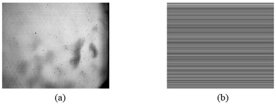
Figure 2. (a) Two-point correction for gain nonuniformity. (b) Two-point correction for bias nonuniformity.

The correction for gain nonuniformity removes the tilt nonuniformity and optically induced fixed-pattern noise of the detector, and the correction for bias nonuniformity removes the streak noise caused by the readout circuit. Real infrared image sequence noise contains tilt nonuniform noise, streak nonuniform noise, and optically induced fixed-pattern noise. We assumed that the nonuniform noise varies with the time drift over a long period of time; however, during each mission of the detector, the nonuniform noise does not change drastically and shows a strong correlation between adjacent frames of the sequence obtained by shooting. We consider that two adjacent images are largely overlapping so that the difference in the pixel gray values between the images is not large, and the corresponding changes in the nonuniform noise are small and can be ignored. We performed time-domain interframe differencing on a real image sequence without denoising, as shown in Figure 3. Therefore, we can use a time-domain difference operator to differentiate the image, utilize the sparsity of noise in the time domain to estimate the noisy image, and finally subtract the two images to obtain the denoised image. The figure shows that the nonuniform noise is basically eliminated and can be ignored in the interframe information. It is evident in Figure 4 that the noise is sparser in the time domain. In addition, for computational convenience, we regarded both the nonuniform noise and fixed-pattern noise caused by the detector optics in the image sequence from the same imaging step as additive noise. Thus, the infrared image degradation model can be expressed mathematically as

$$\mathbf{f}=\mathbf{u}+\mathbf{b}$$

(1)

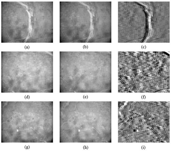
Figure 3. Time-domain interframe differencing of real image sequences without denoising. (a,b,d,e,g,h) depict the denoised real image; (c,f,i) depict the interframe differential image.

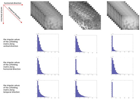
Figure 4. From left to right: the singular values of unfolding matrices of the observed video, the clean video, and the noise.

Here, $\mathbf{f}\in {\mathbf{R}}^{\mathbf{x}\times \mathbf{y}\times \mathbf{t}}$ denotes the measurement image, where x, y, and t denote the number of rows, columns, and frames, respectively; $\mathbf{u}$ is the desired clear image; and $\mathbf{b}$ is the offset, also known as the additive noise component, which consists of streak noise and optically induced fixed-pattern noise. The objective of our study was to estimate both the image with the nonuniform noise and the clear image from the degraded image. Our algorithm incorporates a temporal differential operator into the traditional variational approach, enabling simultaneous removal of multiple types of nonuniform noise—including triangular fixed-pattern noise—thereby better preserving detailed information and reducing the occurrence of ghosting artifacts.

• Group sparsity of the expected noiseless image: For a sequence of images, the expected noiseless image is continuous in the spatial dimension and time-continuous in the temporal dimension; thus, it has the a priori characteristics of spatiotemporal continuity. The expected noise-free image contains dynamic images, although it is not low-rank because of its spatio-temporal continuity [55]. Therefore, the group sparsity of the expected noise-free image is constrained using $L_{2,1}$-paradigm regularization u, which promotes the separation of noisy images from the expected noise-free image.
• Smoothness of the noisy image in the horizontal direction: It is usually assumed that the direction of the readout circuit streak noise is horizontal, and the image is rotated if the streaks appear in the vertical direction. The derivatives of the streak noise and desired noise-free image in the horizontal direction are different, and the derivative of the streak noise in the horizontal direction is sparser than that of the desired noise-free image in Figure 4. Therefore, we used the ${\nabla }_x\left(\mathbf{u}-\mathbf{f}\right)$ parameter of $L_1$ to enhance the Smoothness of the noise in the horizontal direction.
• Smoothness of the desired noise-free image in the vertical direction: The desired noise-free image is segmentally smooth, indicating that the derivatives of each frame in the sequence of infrared images are not densely packed in the vertical and horizontal directions. Horizontal streaks destroy the Smoothness in the vertical direction. The derivatives of the desired noise-free image are sparser in the vertical direction than those of the noisy image in Figure 4. Therefore, the derivative of the streak noise is dense in the horizontal direction. Accordingly, we used the ${\nabla }_y\mathbf{u}$ parameter of $L_1$ to enhance the Smoothness of the desired noise-free image in the vertical direction.
• Smoothness of nonuniform noisy image in the time direction: Because nonuniform noise is additive, the derivative of the noisy image is sparse in the time direction in Figure 4, whereas the derivative of the desired noise-free image is not sparse. Therefore, the ${\nabla }_t\left(\mathbf{u}-\mathbf{f}\right)$ paradigm of $L_1$ is used to enhance the Smoothness of the noisy image in the time direction.

$$\left\{\begin{array}{c}{\nabla }_x\mathbf{u}=u(x+1,y,t)-u(x,y,t)\\ {\nabla }_y\mathbf{u}=u(x,y+1,t)-u(x,y,t)\\ {\nabla }_t\mathbf{u}=u(x,y,t+1)-u(x,y,t)\end{array}\right.$$

${\nabla }_x$, ${\nabla }_y$, ${\nabla }_t$ are the linear operators of the corresponding horizontal, vertical, and time-domain first-order difference operators, respectively.

Based on the above analysis, the optimization model for the nonuniformity correction of infrared images in this study is as follows:

$$arg\underset{\mathbf{u}}{min}{\lambda }_1{\left|\left|\mathbf{u}\right|\right|}_{2,1}+{\lambda }_2{\left|\left|{\nabla }_x(\mathbf{u}-\mathbf{f})\right|\right|}_1+{\lambda }_3{\left|\left|{\nabla }_y\left(\mathbf{u}\right)\right|\right|}_1+{\lambda }_4{\left|\left|{\nabla }_t(\mathbf{u}-\mathbf{f})\right|\right|}_1$$

(2)

where ${\lambda }_1$, ${\lambda }_2$, ${\lambda }_3$, and ${\lambda }_4$ are the weight parameters of the regularization terms.

3.3. Proposed Model

The model presented in this paper is a convex optimization problem that can be solved using a convex optimization algorithm. We adopt an efficient alternating direction method of multipliers (ADMM) algorithm to solve the proposed model. By introducing the variables ${\mathbf{d}}_1$, ${\mathbf{d}}_x$, ${\mathbf{d}}_y$, and ${\mathbf{d}}_t$, we rewrite the proposed model as the following constrained problem:

$$\begin{array}{cc}\hfill & arg\underset{\mathbf{u}}{min}{\lambda }_1{\left|\left|{\mathbf{d}}_1\right|\right|}_{2,1}+{\lambda }_2{\left|\left|{\mathbf{d}}_x\right|\right|}_1+{\lambda }_3{\left|\left|{\mathbf{d}}_y\right|\right|}_1+{\lambda }_4{\left|\left|{\mathbf{d}}_t\right|\right|}_1\hfill \\ \hfill & s.t.{\mathbf{d}}_1=\mathbf{u},{\mathbf{d}}_x={\nabla }_x(\mathbf{u}-\mathbf{f}),{\mathbf{d}}_y={\nabla }_y\left(\mathbf{u}\right),{\mathbf{d}}_t={\nabla }_t(\mathbf{u}-\mathbf{f})\hfill \end{array}$$

(3)

Subsequently, iterations are performed using the Bregman method, and the above equation is further transformed into an unconstrained minimization problem.

$$\begin{array}{cc}\hfill & arg\underset{\mathbf{u},{\mathbf{d}}_1,{\mathbf{d}}_x,{\mathbf{d}}_y,{\mathbf{d}}_t}{min}{\lambda }_1{\left|\left|{\mathbf{d}}_1\right|\right|}_{2,1}+{\lambda }_2{\left|\left|{\mathbf{d}}_x\right|\right|}_1+{\lambda }_3{\left|\left|{\mathbf{d}}_y\right|\right|}_1+{\lambda }_4{\left|\left|{\mathbf{d}}_t\right|\right|}_1+{\displaystyle \frac{{\alpha }_1}{2}}{\left||{\mathbf{d}}_1-\mathbf{u}-{\mathbf{b}}_1|\right|}_2^2\hfill \\ \hfill & +{\displaystyle \frac{{\alpha }_2}{2}}{\left||{\mathbf{d}}_x-{\nabla }_x(\mathbf{u}-\mathbf{f})-{\mathbf{b}}_x|\right|}_2^2+{\displaystyle \frac{{\alpha }_3}{2}}{\left||{\mathbf{d}}_y-{\nabla }_y\mathbf{u}-{\mathbf{b}}_y|\right|}_2^2+{\displaystyle \frac{{\alpha }_4}{2}}{\left||{\mathbf{d}}_t-{\nabla }_t(\mathbf{u}-\mathbf{f})-{\mathbf{b}}_t|\right|}_2^2\hfill \end{array}$$

(4)

${\alpha }_1$, ${\alpha }_2$, ${\alpha }_3$ and ${\alpha }_4$ denote the Bregman penalty coefficient, and the variables ${\mathbf{b}}_1$, ${\mathbf{b}}_x$, ${\mathbf{b}}_y$ and ${\mathbf{b}}_t$ are the intermediate variables identified after Bregman’s iterative determination of the intermediate variables. The solution to the above equation is the alternating minimization method, which transforms the nonuniformity correction model into five simple subproblems by iteratively optimizing one variable while fixing the others.

• The $\mathbf{u}$-related subproblem is as follows.
  The solution of the least squares problem is given by [56]

  $$\begin{array}{cc}\hfill & \underset{\mathbf{u}}{min}{\displaystyle \frac{{\alpha }_1}{2}}{\left||{\mathbf{d}}_1-\mathbf{u}-{\mathbf{b}}_1|\right|}_2^2+{\displaystyle \frac{{\alpha }_2}{2}}{\left||{\mathbf{d}}_x-{\nabla }_x(\mathbf{u}-\mathbf{f})-{\mathbf{b}}_x|\right|}_2^2\hfill \\ \hfill & +{\displaystyle \frac{{\alpha }_3}{2}}{\left||{\mathbf{d}}_y-{\nabla }_y\mathbf{u}-{\mathbf{b}}_y|\right|}_2^2+{\displaystyle \frac{{\alpha }_4}{2}}{\left||{\mathbf{d}}_t-{\nabla }_t(\mathbf{u}-\mathbf{f})-{\mathbf{b}}_t|\right|}_2^2\hfill \end{array}$$

  (5)
  As it is a convex function, it is equal to the following linear system:

  $$\begin{array}{cc}\hfill & ({\alpha }_1+{\alpha }_2{\nabla }_x^T{\nabla }_x+{\alpha }_3{\nabla }_y^T{\nabla }_y+{\alpha }_4{\nabla }_t^T{\nabla }_t){\mathbf{u}}^{k+1}=\hfill \\ \hfill & ({\alpha }_1\times {\mathbf{d}}_1^k-{\mathbf{b}}_1^k+{\alpha }_2{\nabla }_x^T({\mathbf{d}}_x^k+{\nabla }_x\mathbf{f}-{\mathbf{b}}_x^k)+{\alpha }_3{\nabla }_y^T({\mathbf{d}}_y^k-{\mathbf{b}}_y^k)+{\alpha }_4{\nabla }_t^T({\mathbf{d}}_t^k+{\nabla }_t\mathbf{f}-{\mathbf{b}}_t^k))\hfill \end{array}$$

  (6)
  In the above equation, the superscript T is the matrix transpose operator and k is the number of iterations for solving the above equation, which can be computed using the closed solution of the fast Fourier transform (FFT).

  $$\begin{array}{c}\hfill {\mathbf{u}}^{k+1}={\mathcal{F}}^{-1}\left({\displaystyle \frac{R}{S}}\right)\end{array}$$

  (7)
  We make
  $R=({\alpha }_1\times {\mathbf{d}}_1^k-{\mathbf{b}}_1^k+{\alpha }_2{\nabla }_x^T({\mathbf{d}}_x^k+{\nabla }_x\mathbf{f}-{\mathbf{b}}_x^k)+{\alpha }_3{\nabla }_y^T({\mathbf{d}}_y^k-{\mathbf{b}}_y^k)+{\alpha }_4{\nabla }_t^T({\mathbf{d}}_t^k+{\nabla }_t\mathbf{f}-{\mathbf{b}}_t^k))$,
  $S=({\alpha }_1\times I+{\alpha }_2{\left(\mathcal{F}\left({\nabla }_x\right)\right)}^2+{\alpha }_3{\left(\mathcal{F}\left({\nabla }_y\right)\right)}^2+{\alpha }_4{\left(\mathcal{F}\left({\nabla }_t\right)\right)}^2)$
  and where I is the unit matrix, $\mathcal{F}(·)$ is the fast Fourier transform, and ${\mathcal{F}}^{(-1)}(·)$ is the fast Fourier inverse transform.
• The ${\mathbf{d}}_1$-related subproblem is

  $$\underset{{\mathbf{d}}_1}{min}{\lambda }_1{\left|\left|{\mathbf{d}}_1\right|\right|}_{2,1}+{\displaystyle \frac{{\alpha }_1}{2}}{\left||{\mathbf{d}}_1-\mathbf{u}-{\mathbf{b}}_1|\right|}_2^2$$

  (8)

  which is equivalent to

  $$\underset{{\mathbf{d}}_1}{min}\sum _{g_i}({\lambda }_1{\left|\left|{\mathbf{d}}_{1g_i}\right|\right|}_2+{\displaystyle \frac{{\alpha }_1}{2}}{\left||{\mathbf{d}}_{1g_i}-{\mathbf{u}}_{g_i}-{\mathbf{b}}_{1g_i}|\right|}_2^2)$$

  (9)
  The above equation can be computed using a soft threshold operator as follows:

  $${\mathbf{d}}_{1g_i}^{k+1}=Shrink({\mathbf{u}}_{1g_i}^{k+1}+{\mathbf{b}}_{1g_i}^k,{\displaystyle \frac{{\lambda }_1}{{\alpha }_1}})$$

  (10)

  where $Shrink(·)$ is the soft thresholding operation.

  $$Shrink(r,\xi )={\displaystyle \frac{r}{\left|r\right|}}\times max(r-\xi ,0)$$

  (11)
• The ${\mathbf{d}}_x$-related subproblem is

  $$\underset{{\mathbf{d}}_x}{min}{\lambda }_2{\left|\left|{\mathbf{d}}_x\right|\right|}_1+{\displaystyle \frac{{\alpha }_2}{2}}{\left||{\mathbf{d}}_x-{\nabla }_x(\mathbf{u}-\mathbf{f})-{\mathbf{b}}_x|\right|}_2^2$$

  (12)
  The above equation can be similarly solved as

  $${\mathbf{d}}_x^{k+1}=Shrink({\nabla }_x({\mathbf{u}}^{k+1}-\mathbf{f})+{\mathbf{b}}_x^k,{\displaystyle \frac{{\lambda }_2}{{\alpha }_2}})$$

  (13)
• The ${\mathbf{d}}_y$-related subproblem is

  $$\underset{{\mathbf{d}}_y}{min}{\lambda }_3{\left|\left|{\mathbf{d}}_y\right|\right|}_1+{\displaystyle \frac{{\alpha }_3}{2}}{\left||{\mathbf{d}}_y-{\nabla }_y\mathbf{u}-{\mathbf{b}}_y|\right|}_2^2$$

  (14)
  The above equation can be similarly solved as

  $${\mathbf{d}}_y^{k+1}=Shrink({\nabla }_y{\mathbf{u}}^{k+1}+{\mathbf{b}}_y^k,{\displaystyle \frac{{\lambda }_3}{{\alpha }_3}})$$

  (15)
• The ${\mathbf{d}}_t$-related subproblem is

  $$\underset{{\mathbf{d}}_t}{min}{\lambda }_4{\left|\left|{\mathbf{d}}_t\right|\right|}_1+{\displaystyle \frac{{\alpha }_4}{2}}{\left||{\mathbf{d}}_t-{\nabla }_t(\mathbf{u}-\mathbf{f})-{\mathbf{b}}_t|\right|}_2^2$$

  (16)
  The above equation can be similarly solved as

  $${\mathbf{d}}_t^{k+1}=Shrink({\nabla }_t({\mathbf{u}}^{k+1}-\mathbf{f})+{\mathbf{b}}_t^k,{\displaystyle \frac{{\lambda }_4}{{\alpha }_4}})$$

  (17)

The Lagrange multiplier is updated by the following equation:

$$\left\{\begin{array}{c}{\mathbf{b}}_1^{k+1}={\mathbf{b}}_1^k+({\nabla }_t({\mathbf{u}}^{k+1}-\mathbf{f})-{\mathbf{d}}_1^{k+1})\hfill \\ {\mathbf{b}}_x^{k+1}={\mathbf{b}}_x^k+({\nabla }_x({\mathbf{u}}^{k+1}-\mathbf{f})-{\mathbf{d}}_x^{k+1})\hfill \\ {\mathbf{b}}_y^{k+1}={\mathbf{b}}_y^k+({\nabla }_y{\mathbf{u}}^{k+1}-{\mathbf{d}}_y^{k+1})\hfill \\ {\mathbf{b}}_t^{k+1}={\mathbf{b}}_t^k+({\nabla }_t({\mathbf{u}}^{k+1}-\mathbf{f})-{\mathbf{d}}_t^{k+1})\hfill \end{array}\right.$$

(18)

Because the proposed model is convex and the variables can be split into multiple groups, the convergence of the proposed algorithm is theoretically guaranteed in the ADMM framework.

In conclusion, the advantage of the split Bregman method is that the challenging optimization problem in Equation (1) is decomposed into the five subproblems mentioned above, which are relatively easy to optimize. The u-subproblem is efficiently accelerated using the FFT, and the ${\mathbf{d}}_1-$,${\mathbf{d}}_x-$, ${\mathbf{d}}_y-$, and ${\mathbf{d}}_t-$subproblems are solved using efficient soft contraction operators. Moreover, the ${\mathbf{d}}_1-$,${\mathbf{d}}_x-$, ${\mathbf{d}}_y-$, and ${\mathbf{d}}_t-$subproblems are independent and can be computed efficiently in parallel. Subsequently, ${\mathbf{b}}_1$, ${\mathbf{b}}_x$, ${\mathbf{b}}_y$, and ${\mathbf{b}}_t$ can be updated in parallel. Figure 5 and Algorithm 1 summarizes the flow of the nonuniformity correction process.

Algorithm 1: Proposed Method

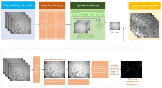
Figure 5. Schematic Diagram of the Complete Algorithm.

4. Results

4.1. Preprocessing

The in-orbit operation of a satellite is affected by the photon effect, temperature changes, time drift, and other factors; the response characteristics of the infrared focal plane array will drift, and the use of ground calibration of the data will cause a certain deviation, resulting in an infrared focal plane array of blind elements and the nonuniformity of the noise becoming more serious. The existence of blind elements will cause fixed white and black dots in the infrared focal plane array imaging, thus affecting the visual effect of the image. Because the real validation of this algorithm is based on the images collected by the infrared camera of the satellite in orbit, the blind elements need to be processed; otherwise, the subsequent nonuniformity correction algorithm will be affected to some extent. We improved the method for removing blind elements in a previous study [57].

In the infrared image sequence is $f(i,j,t)$, where t is the frame number; $(i,j)$ represents the horizontal and vertical coordinates of the infrared focal plane pixels; $[i=1,2,\dots ,m]$, $[j=1,2,\dots ,n]$,$[t=1,2,\dots ,T]$; m and n denote the number of rows and columns in each image, respectively; and T denotes the total number of frames in the infrared image sequence. Firstly, to determine the time-domain mean value of each pixel point

$$B_{tavg}(i,j)={\displaystyle \frac{{\sum }_{N=1}^{k}f(i,j,N)}{k}}(k\le T)$$

(19)

an infrared image sequence with a frame number of T is computed as a single time-domain mean image, and based on experience, k can be taken to be either 10 or 20, which reduces the amount of computation.

We used local nonlinear filtering with a sliding window of 3 × 3, in which the maximum and minimum values within the window were removed from the sliding window of the image, and the sum of the time-domain mean values of each pixel in the window was computed with the time-domain maxima and minima in the window. $\overline{B(i,j)}$ denotes the cumulative subtraction of the maxima and minima of the time-domain means of the time-domain mean images within the square proximity centered at $(i,j)$; N is the side length of this square proximity of image elements and takes the value of three image elements; $B_{max}$ is the maximum value in the square proximity centered at $(p\pm N,q\pm N)$; and $B_{min}$ is its minimum value.

$$\overline{B(i,j)}={\displaystyle \frac{V}{N^2-2}}$$

(20)

We make

$V={\sum }_{p=\left({\displaystyle \frac{-(N-1)}{2}}\right)}^{{\displaystyle \frac{(N-1)}{2}}}{\sum }_{q=\left({\displaystyle \frac{-(N-1)}{2}}\right)}^{{\displaystyle \frac{(N-1)}{2}}}{B}_{tavg}(i+p,j+p)-B_{max}-B_{min}$, and the local mean $\overline{B(i,j)}$ of the obtained window is used to compute the threshold for judging the blind elements.

$$delta1={\displaystyle \frac{B_{tavg}(i,j)-\overline{B(i,j)}}{\overline{B(i,j)}}}$$

(21)

$$delta2={\displaystyle \frac{\overline{B(i,j)}-B_{tavg}(i,j)}{\overline{B(i,j)}}}$$

(22)

The infrared focal plane image element (i,j) is judged to be a blind metapoint when the threshold $delta1\ge 0.1$ or $delta2\ge 0.1$, $blind(i,j)=1$.

Points with $blind(i,j)=1$ are compensated for their blind elements using the mean filtering method.

$$f(i,j,t)=mean\left({\displaystyle \frac{{\sum }_{p=\left(\frac{-(N-1)}{2}\right)}^{\frac{(N-1)}{2}}{\sum }_{q=\left(\frac{-(N-1)}{2}\right)}^{\frac{(N-1)}{2}}f(i+p,j+p)}{N^2}}\right)$$

(23)

4.2. Experimental Parameter Setting

We compared the proposed method with several state-of-the-art methods for removing nonuniform noise, namely, Adjacency Difference Statistics (ADS) [8], Constant Statistics of Adjacency Ratios (CSAR) [4], Reweighted Block Sparsity Regularization (RBS) [51], FPN Estimation (FPNE) [7], FastHyMix (FHM) [58], flexible and effective U-shaped network (FEU) [35], Stripe Estimation and Image Denoising framework (SEID) [47], Multi-Domain Infrared Video Denoising network (MDIVD) [59], Asymmetric Sampling Correction network (ASCNet) [60] and Unicd [36]. The SEID is currently an advanced TV algorithm and the Unicd is the most advanced neural-network-based algorithm. The first two algorithms remove streak nonuniform noise, and the last three eliminate other types of nonuniform noise. To minimize boundary effects, we added five filler elements to the image sequence in each dimension of the 3D tensor. Thus, the size of the resulting input tensor was $(m+10)\times (n+10)\times (t+10)$. In the proposed method, ${\alpha }_1$, ${\alpha }_2$, ${\alpha }_3$, and ${\alpha }_4$ were set to [1,500],[1,500], [1,500], and [1,500], respectively. Based on experience, we set ${\alpha }_1$ = 100, ${\alpha }_2$ = 100, ${\alpha }_3$ = 5, ${\alpha }_4$ = 100. In addition, we set ${\lambda }_1$ = ${\lambda }_2$ = ${\lambda }_3$ = ${\lambda }_4$ = 50. $ite{m}_{max}$ was set to 200. Through experimentation, we obtained the convergence curve for ADMM in Figure 6. It can be observed that when $\epsilon$ = 0.001, mean NIQE (M_NIQE) converges and reaches its maximum value, demonstrating the best performance. Therefore, we set $\epsilon$ = 0.001.

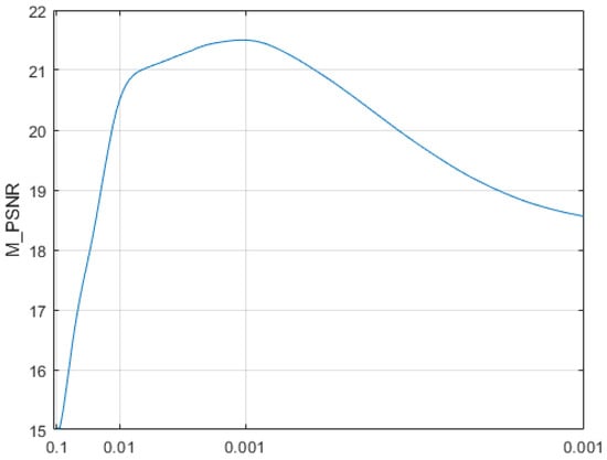
Figure 6. M_PSNR Values of ADMM at Different $\epsilon$ Values.

In the case of the RBS, FPNE, and ADS algorithms, the following parameters reported in their respective papers were used: lamda1 = 0.1, lamda2 = 0.5 for the RBS algorithm; $T_{max}$ = 350, $T_{min}$ = 25, $N_1$ = 10, $N_2$ = 50, and alpha = 0.3 for the FPNE algorithm; the ADS algorithm used L = 33, K = 3; the ASCNet algorithm set the basic width to 32, and the channel expansion factor $\theta$ in three RHDWTs is set to 2, 2, and 1 separately; and the MDIVD algorithm used hyperparameters n = 5, p = 5, and $N_{\varphi }$ = 5.

4.3. Simulation Experiment

Our method uses a time difference operator that requires continuous multi-frame video data images. Therefore, we chose a publicly available space-based remote sensing video dataset [61] for simulation validation, as shown in Figure 7, whose data collects 200 sets of continental and terrestrial ocean images in the seventh band of Landsat 8 and 9, at SWIR wavelengths of 2.1–2.3 µm, and whose image size we set to be 320 × 256, and each video has more than 300 frames. The dataset comprises 200 sequences and 90,000 image frames. To eliminate invalid background interference, we excluded 37 sequences with pure black backgrounds (containing 19,237 images). The final experimental dataset utilized approximately 160 sequences, totaling around 70,000 images.

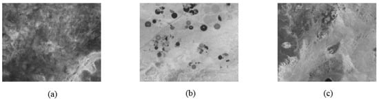
Figure 7. (a–c) Clear images were used to generate to the simulation dataset.

We added streak nonuniformity and optically induced fixed-pattern noise superposition in the simulation. Regarding nonuniform noise, we consider that for two adjacent images with substantial partial overlap and a similar distribution of image gray values, their corresponding nonuniform noise variations are small and can be ignored; thus, they are similar to additive noise.

We used a random horizontal stripe noise of intensity K and rotated it by 0°, 60°, and 120°, superimposed on each other as nonuniform noise, as a way to simulate the triangular fixed-pattern noise. Based on experience, the noise intensity K was set to 15 and 25.

$$nois{e}_{temp}={\displaystyle \frac{K}{2\ast 100\ast \pi }}{e}^{{\displaystyle \frac{-{(x-\frac{m}{2})}^2-{(y-\frac{n}{2})}^2}{2\ast {100}^2}}}$$

(24)

By using the center point of the image as the starting point, we set it to be optically induced fixed-pattern noise by using a Gaussian distribution probability density function Equation (24) and using the distances of the other pixel points from the center point of the image as random variables of the Gaussian distribution probability density function. x and y are the distances of the pixel points from the center point of the image, m and n denote the number of rows and columns in each image.

Qualitative and quantitative metrics were used to evaluate the quality of the recovered images. The qualitative evaluation was conducted using the visualization results; in addition, two objective positive full-reference quality metrics were chosen as the quantitative metrics because of the use of real images in the simulation experiments: structural similarity index measure (SSIM) [62,63] and peak signal-to-noise ratio (PSNR) [64,65]. PSNR describes the difference between the pixels of the denoised and real images, and SSIM describes the similarity between them. We used a publicly available thermal infrared sequence dataset with a resolution of 320 × 256 and selected multiple sequences from multiple scenes, each containing 300 frames of continuously captured images. Unlike traditional single-frame algorithms, the method proposed in this paper is based on a temporal difference operator, which relies on video sequences to obtain time-domain difference information for computation. To align with this characteristic and ensure evaluation accuracy, the performance metrics for each scenario in the experiments are calculated using the average values of the corresponding video sequence images. Given the massive scale of the video sequence data, we selected one representative frame from each sequence for display. We then calculated the values of the mean SSIM (M_SSIM) and mean PSNR (M_PSNR) across all images within each sequence, using these as quantitative metrics for evaluating algorithm performance.

We used different intensities of noise to test the first sequence. It was almost impossible to remove the nonuniform noise using the traditional nonuniformity correction method. The results of the evaluation at K = 15 are shown in Figure 8. At K = 15, the RBS and SEID algorithms cannot remove noise. The FEU, ASCnet, and MDIVD algorithms could remove only the horizontal stripes, whereas CSAR could not completely remove the noise; that is, the denoised real image contained some noise. The FPNE, ADS and FHM algorithms effectively removed the noise, but there was an obvious noise residue, appearing as white or black residual ghosts in the image. Therefore, these methods lag behind the proposed algorithms in terms of the evaluation index.

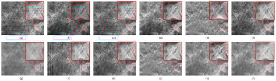
Figure 8. Nonuniformity correction results for the scene 1 with simulation noise intensity K = 15. (a) Image with simulated nonuniformity. Results of (b) CSAR, (c) RBS, (d) FPNE, (e) FHM, (f) FEU, (g) SEID, (h) MDIVD, (i) ASC, (j) Unicd, (k) the proposed method, and (l) Ground Truth.

The results of the evaluation at K = 25 are shown in Figure 9. At K = 25, the RBS and SEID algorithms cannot remove noise.The FEU, ASCnet, and MDIVD gave the same results as before and only the horizontal streaks were removed. The effects of the CSAR, FPNE, and FHM algorithms were not as significant as those at K = 15, and the ADS algorithm continued to show artifactual ghosting, although there was no noise residue. In terms of the evaluation metrics, the proposed algorithm achieved better results.

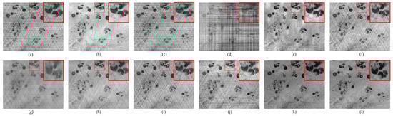
Figure 9. Nonuniformity correction results for the scene 2 with simulation data, noise intensity K = 15. (a) Image with simulated nonuniformity. Results of (b) CSAR, (c) RBS, (d) FPNE, (e) FHM, (f) FEU, (g) SEID, (h) MDIVD, (i) ASC, (j) Unicd, (k) the proposed method, and (l) Ground Truth.

The second scenario was also tested using nonuniform noise with noise intensities of K = 15 and K = 25 (Figure 10 and Figure 11, respectively). At K = 15, we found that the RBS and SEID algorithms cannot remove noise, the FEU, ASCnet, and MDIVD removed only the horizontal streaks, as before. The CSAR, FPNE, and FHM algorithms had obvious noise residuals, whereas the ADS algorithm had no noise residuals, yet showed greater artifactual ghosting.

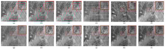
Figure 10. Nonuniformity correction results for the scene 3 with simulation noise intensity K = 15. (a) Image with simulated nonuniformity. Results of (b) CSAR, (c) RBS, (d) FPNE, (e) FHM, (f) FEU, (g) SEID, (h) MDIVD, (i) ASC, (j) Unicd, (k) the proposed method, and (l) Ground Truth.

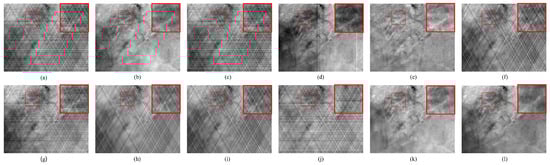
Figure 11. Nonuniformity correction results for the scene 4 with simulation noise intensity K = 15. (a) Image with simulated nonuniformity. Results of (b) CSAR, (c) RBS, (d) FPNE, (e) FHM, (f) FEU, (g) SEID, (h) MDIVD, (i) ASC, (j) Unicd, (k) the proposed method, and (l) Ground Truth.

We compared the results for K = 15 and K = 25 for the second scenario; the results were found to be approximately the same. It is worth mentioning that the M_SSIM and M_PSNR of our algorithm were not as pronounced as those of the other algorithms when the noise intensity of the two scenes was large (Table 2). This indicates a certain boundedness to our algorithm when the noise is large; moreover, the evaluation metrics were poorer and not as significant as those at K = 15.

Table 2. M_SSIM and M_PSNR results of different methods applied to simulated nonuniform noise images. (The upward arrow indicates that higher values are better for the metric. Red represents the optimal algorithm, while blue indicates the next best).

Noise Case	Index	CSAR	RBS	FPNE	FHM	FEU	SEID	MDIVD	ASC	UniCD	Ours
scene 1	M_SSIM ↑	0.863	0.388	0.886	0.890	0.791	0.461	0.567	0.483	0.478	0.897
K = 15	M_NIQE ↑	15.223	18.611	17.087	19.486	18.611	18.812	19.861	18.872	19.012	20.058
scene 1	M_SSIM ↑	0.838	0.238	0.769	0.779	0.791	0.367	0.329	0.315	0.451	0.893
K = 25	M_NIQE ↑	15.585	16.468	18.392	19.434	16.571	17.812	17.422	17.018	18.781	19.691
scene 2	M_SSIM ↑	0.906	0.433	0.662	0.886	0.801	0.517	0.680	0.561	0.310	0.935
K = 15	M_NIQE ↑	17.610	20.004	17.005	19.933	20.181	20.124	20.107	22.251	16.917	22.813
scene 2	M_SSIM ↑	0.870	0.268	0.606	0.852	0.803	0.422	0.506	0.381	0.489	0.934
K = 25	M_NIQE ↑	15.792	17.118	17.222	19.956	19.988	16.815	19.975	20.002	19.186	20.520
scene 3	M_SSIM ↑	0.892	0.382	0.580	0.797	0.759	0.481	0.563	0.465	0.412	0.915
K = 15	M_NIQE ↑	18.389	19.796	17.966	19.950	20.192	20.089	20.163	20.327	19.867	21.818
scene 3	M_SSIM ↑	0.837	0.213	0.555	0.786	0.761	0.391	0.300	0.256	0.261	0.915
K = 25	M_NIQE ↑	15.336	17.087	17.721	19.890	19.211	18.911	19.409	19.760	18.714	20.272
scene 4	M_SSIM ↑	0.858	0.242	0.853	0.812	0.841	0.284	0.512	0.263	0.901	0.909
K = 15	M_NIQE ↑	20.120	14.811	17.469	15.267	16.817	15.442	20.948	20.739	22.405	26.129
scene 4	M_SSIM ↑	0.882	0.168	0.877	0.805	0.814	0.183	0.502	0.161	0.863	0.892
K = 25	M_NIQE ↑	18.952	12.878	19.179	13.867	14.781	13.996	20.602	20.698	23.068	24.925
scene 5	M_SSIM ↑	0.373	0.357	0.848	0.383	0.412	0.406	0.532	0.838	0.807	0.862
K = 15	M_NIQE ↑	11.217	17.675	21.616	16.604	16.891	17.522	21.815	22.120	21.741	25.858
scene 5	M_SSIM ↑	0.493	0.251	0.868	0.279	0.265	0.286	0.499	0.809	0.804	0.881
K = 25	M_NIQE ↑	12.859	15.579	21.524	16.604	16.891	13.998	20.545	21.410	21.063	24.909
scene 6	M_SSIM ↑	0.881	0.314	0.882	0.383	0.416	0.377	0.491	0.795	0.825	0.873
K = 15	M_NIQE ↑	19.152	14.18	20.265	17.381	18.012	14.424	21.709	24.843	19.17	25.574
scene 6	M_SSIM ↑	0.854	0.214	0.877	0.256	0.291	0.262	0.495	0.789	0.805	0.859
K = 25	M_NIQE ↑	18.285	14.264	20.238	17.104	17.831	14.957	20.736	24.278	19.088	25.040

The results of the third scenario are similar to those of the second scenario, with other algorithms still leaving noise or producing ghosting. We compared the results for K = 15 and K = 25 for the third scenario (Figure 12 and Figure 13, respectively), and compared to the comparison algorithms, our algorithm still achieves satisfactory results on the eye and metrics, proving that our algorithm is still effective on the simulated remote sensing dataset. The figure (Table 2) shows the M_PSNR and M_SSIM values obtained from video sequences across multiple scenarios—six simulated scenarios under two different noise intensities. We highlight the best metrics in red and the next-best metrics in blue. The quantitative evaluation results of the Simulation datasets are shown in Figure 14, from which it can be found that our proposed method has better performance. The bar chart in the table represents the mean, and the lines within the bars represent the standard deviation.

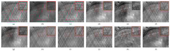
Figure 12. Nonuniformity correction results for the scene 5 with simulation noise intensity K = 15. (a) Image with simulated nonuniformity. Results of (b) CSAR, (c) RBS, (d) FPNE, (e) FHM, (f) FEU, (g) SEID, (h) MDIVD, (i) ASC, (j) Unicd, (k) the proposed method, and (l) Ground Truth.

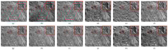
Figure 13. Nonuniformity correction results for the scene 6 with simulation noise intensity K = 15. (a) mage with simulated nonuniformity. Results of (b) CSAR, (c) RBS, (d) FPNE, (e) FHM, (f) FEU, (g) SEID, (h) MDIVD, (i) ASC, (j) Unicd, (k) the proposed method, and (l) Ground Truth.

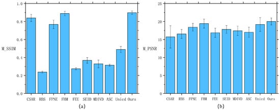
Figure 14. Quantitative comparison on the simulation datasets evaluated by (a) M_SSIM and (b) M_PSNR.

4.4. Real Experiment

We used the real data obtained from the infrared camera on board the Qilu-2 satellite to verify the effectiveness of the proposed method. The Qilu-2 satellite is a lightweight Earth observation satellite equipped with a dual-mode imaging payload operating in visible light and longwave infrared. The visible light channels comprise four spectral bands: panchromatic, blue, green, and red. Operating at an altitude of 500 km, the satellite achieves imaging frame rates of 20 frames per second for visible light and 25 frames per second for longwave infrared. The infrared camera of the satellite is a face-array detector covering the long-wave infrared from 7.7 µm to 11.7 µm. It has a high resolution of 16 m and width of 4.4 km. The image size is 320 × 256 with 350 groups of Earth cities and ocean backgrounds, and each video has 280 frames [66]. The image data used in this study’s practical validation were directly sourced from raw satellite-transmitted decoded data and did not undergo radiometric calibration or other radiometric preprocessing steps. Owing to the various factors affecting the face-array detector during the orbiting operation, nonuniform noise, which is optically induced by fixed-pattern noise, is severe. In addition, the intensity of the nonuniform noise in the real image was lower than that in the simulated data, but the pattern was more complex. It was not possible to obtain clear noise-free images in the experiments, as in the simulated data.

Therefore, we used the nonreference evaluation metrics, mean relative deviation (MRD) [40,44], and natural image quality evaluator (NIQE) [67,68] to quantitatively evaluate the processing results. We selected one representative frame from each video sequence for display. Subsequently, we calculated the mean MRD (M_MRD) and mean NIQE(M_NIQE) for all images within each sequence, using these as quantitative metrics to evaluate algorithm performance.

$$MRD={\displaystyle \frac{1}{N}}\sum _{i=1}^N\left|{\displaystyle \frac{I_i^{rec}-I_i^{ori}}{I_i^{ref}+\epsilon }}\right|$$

(25)

Here, $I_i^{rec}$ and $I_i^{ori}$ denote the gray values of the i-th pixel in the de-stripe image and the original image, respectively. N is the total number of pixels within the evaluation region, and $\epsilon$ is a very small constant (e.g., ${10}^{-8}$) used to prevent division by zero. A smaller MRD value indicates lower relative error, meaning the restored image is closer to the reference image, which is the stripe image.

The M_MRD and M_NIQE values were used to assess the recovery of the image sequence. Lower M_MRD and M_NIQE values indicate better image recovery quality. We selected six sets of images acquired at different locations and times.

Tests on the real infrared data of Qilu-2 showed that the RBS, SEID, FEU, ASCNet, MDIVD and UniCD algorithms were not effective in removing the nonuniform noise, as shown in Figure 15. The FPNE algorithm could remove the nonuniform noise; due to the nature of its algorithm, FPNE is only effective in certain scenarios. When images contain backgrounds such as cities and oceans simultaneously, its noise reduction performance is suboptimal. The CSAR, ADS and FHM algorithms could remove the nonuniform noise, but from a quantitative perspective, its M_MRD and M_NIQE indexes were higher than those of the proposed algorithms, i.e., the quality of its corrected real image was lower than that of the proposed algorithm.

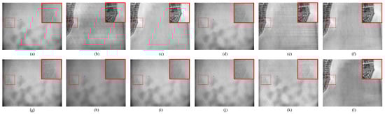
Figure 15. Nonuniformity correction results for the scene 1 with real data. (a) Image with real nonuniformity. Results of (b) ADS, (c) CSAR, (d) RBS, (e) FPNE, (f) FHM, (g) FEU, (h) SEID, (i) MDIVD, (j) ASC, (k) UniCD and (l) the proposed method.

We repeated the experiment with another set of acquired images, and the results are shown in Figure 16. It can be seen that the performances of the RBS, SEID, FEU, ASCNet, MDIVD and UniCD algorithms remained unsatisfactory for the removal of nonuniform noise. Our proposed algorithm showed the best results among the compared algorithms in both the eye examination and quantitative analysis.

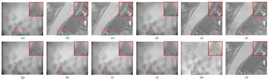
Figure 16. Nonuniformity correction results for the scene 2 with real data. (a) Image with real nonuniformity. Results of (b) ADS, (c) CSAR, (d) RBS, (e) FPNE, (f) FHM (g) FEU, (h) SEID, (i) MDIVD, (j) ASC, (k) UniCD and (l) the proposed method.

For the third group of images in Figure 17, the RBS, SEID, FEU, ASCNet, MDIVD, and UniCD algorithms were not effective in removing the nonuniform noise, and low-contrast scenes were observed; that is, the upper and lower limits of the gray value of the image did not differ noticeably. The FPNE algorithm could remove only part of the nonuniform noise, and streak noise was still present. The CSAR, ADS and FHM algorithms showed obvious residual ghosting, but our proposed algorithm achieved better processing results.

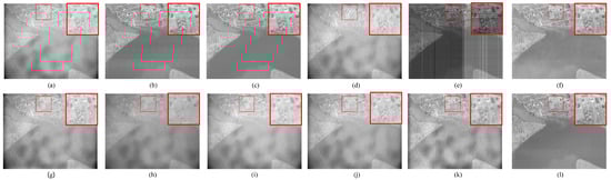
Figure 17. Nonuniformity correction results for the scene 3 with real data. (a) Image with real nonuniformity. Results of (b) ADS, (c) CSAR, (d) RBS, (e) FPNE, (f) FHM, (g) FEU, (h) SEID, (i) MDIVD, (j) ASC, (k) UniCD and (l) the proposed method.

The results are shown in Table 3 and Figure 18. We highlight the best metrics in red and the next-best metrics in blue. To comprehensively evaluate algorithm performance, we randomly selected ten video sequences and calculated the M_MRD values, M_NIQE values, and their corresponding standard deviations across ten different scenarios. The quantitative evaluation real datasets results are shown in Figure 18. The bar chart in the table represents the mean, and the lines within the bars represent the standard deviation. Comprehensive analysis indicates that our proposed algorithm achieves the best performance across all evaluation metrics, significantly outperforming the comparison methods. Specifically, this method effectively suppresses ghosting artifacts while better preserving image detail information, demonstrating superior overall restoration capability.

Table 3. M_MRD and M_NIQE results of different methods applied to real noisy infrared images. The downward arrow indicates that lower values are better for the metric. Red represents the optimal algorithm, while blue indicates the next best.

Image	Index	ADS	CSAR	RBS	FPNE	FHM	FEU	SEID	MDIVD	ASC	UniCD	Ours
scene 1	M_MRD ↓	0.219	0.052	0.058	0.338	0.229	0.042	0.084	0.066	0.024	0.065	0.021
	M_NIQE ↓	9.705	5.140	10.562	7.475	5.189	7.981	5.191	7.050	8.812	6.929	4.989
scene 2	M_MRD ↓	0.241	0.039	0.045	0.254	0.576	0.063	0.092	0.419	0.014	0.478	0.009
	M_NIQE ↓	6.989	7.153	11.927	6.757	7.254	7.912	8.916	7.136	11.599	8.781	6.491
scene 3	M_MRD ↓	0.241	0.063	0.050	0.229	0.221	0.059	0.068	0.030	0.023	0.167	0.019
	M_NIQE ↓	6.475	6.889	11.511	6.231	6.888	9.552	10.981	7.056	11.375	7.012	6.444
scene 4	M_MRD ↓	0.244	0.431	0.049	0.236	0.256	0.271	0.048	0.038	0.026	0.179	0.014
	M_NIQE ↓	5.720	5.844	10.426	5.768	5.785	5.836	8.699	7.178	10.203	6.495	5.702
scene 5	M_MRD ↓	0.245	0.055	0.036	0.306	0.311	0.285	0.052	0.039	0.026	0.195	0.019
	M_NIQE ↓	5.128	5.121	10.252	5.083	5.205	5.191	9.773	6.536	11.590	6.046	5.071
scene 6	M_MRD ↓	0.243	0.056	0.054	0.199	0.194	0.215	0.053	0.039	0.024	0.146	0.013
	M_NIQE ↓	5.413	5.523	10.143	5.484	5.525	5.639	7.779	7.861	9.189	5.832	5.328

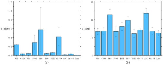
Figure 18. Quantitative comparison on the real datasets evaluated by (a) M_MRD and (b) M_NIQE.

4.5. Ablation Study

To analyze the impacts of different components of each regularization term in our method, we conducted a series of ablation experiments. The ablation study is performed on the simulation datasets. The ablation study mainly contains four cases, i.e., the following: (1) removing Group sparsity of the expected noiseless image (“$D_{xyt}$”); (2) removing Smoothness of noisy image in the horizontal direction (“$D_{1yt}$”); (3) removing Smoothness of the desired noise-free image in the vertical direction (“$D_{1xt}$”); and (4) removing Smoothness of nonuniform noisy image in the time direction (“$D_{1xy}$”). The results shown in Table 4 verify the effectiveness of the given method.

Table 4. Quantitative evaluation results of ablation experiments.

Method	Group Sparsity of u	Smoothness of f in the x Domain	Smoothness of u in the y Domain	Smoothness of f in the Time Domain	M_PSNR	M_SSIM	Δ PSNR	Δ SSIM
$D_{xyt}$	×	✓	✓	✓	15.5345	0.182	−5.9678	−0.735
$D_{lyt}$	✓	×	✓	✓	20.3599	0.761	−1.1424	−0.156
$D_{lxt}$	✓	✓	×	✓	19.6093	0.591	−1.893	0.326
$D_{lxy}$	✓	✓	✓	×	17.4622	0.367	−4.0401	−0.55
Ours	✓	✓	✓	✓	21.5023	0.917	-	-

We have listed the $\Delta$PSNR/$\Delta$SSIM values after comparing the ablation experiments with the complete model. Directional smoothing is primarily used to suppress striped non-uniformity noise appearing in the horizontal direction. This noise mainly originates from the sensor’s readout circuit structure. Due to the row–column arrangement of the readout circuit, its non-uniformity typically manifests as horizontal striped noise in the image. The combined effects of group sparsity and temporal Smoothness regularization targets triangular fixed pattern noise (FPN) within images, as well as FPN caused by optical systems. This type of noise is primarily associated with response inconsistencies within the camera, stemming from factors like uneven thermal distribution, and falls under the category of fixed pattern non-uniformity. Group sparsity facilitates modeling sparse noise structures, while temporal Smoothness constrains fixed-pattern components by leveraging stability across consecutive frames. This approach capitalizes on the noise’s spatially smooth structure: group sparsity models its spatial correlation and stability across multiple consecutive frames, while temporal Smoothness constrains its temporal invariance, enabling separation from dynamically varying real-world scene signals. Together, they synergistically enhance the model’s ability to correct fixed-pattern noise.

4.6. Parametric Analysis

We used the simulation image to analyze and test different parameters according to the PSNR value of the algorithm. We set ${\alpha }_1$ as [1,500], ${\alpha }_3$ as [1,500], and ${\alpha }_4$ as [1,500]. ${\alpha }_2$ was set to [1,500] but with the opposite tendency to that of other parameters, We also set ${\lambda }_1$ = ${\lambda }_2$ = ${\lambda }_3$ = ${\lambda }_4$ as [1,500] and set ${\alpha }_1$ = ${\alpha }_2$ = ${\alpha }_3$ = ${\alpha }_4$ = 100. We used the obtained mean PSNR as an evaluation index and plotted the image (Figure 19a,b). The curve fluctuation was not very large, and when ${\alpha }_1$ and ${\alpha }_2$ take similar values, the PSNR obtained is smaller and the image is not fully recovered, but larger or smaller parameters will lead to over-sharpening of the image. Hence, in our experiments, setting ${\lambda }_1$ = ${\lambda }_2$ = ${\lambda }_3$ = ${\lambda }_4$ = 50 yielded better results.

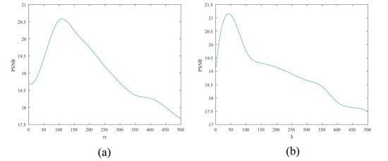
Figure 19. (a) Relationship between PSNR and the parameter $\alpha$. (b) Relationship between PSNR and the parameter $\lambda$.

Experiments demonstrate that parameter variations exert a measurable influence on solution outcomes. However, parameter selection relies more on the model’s construction methodology and noise type than on noise intensity. This paper employs identical parameter settings across both simulation and real-world experiments. Although the noise intensity configured in simulations differs from real-world scenarios, this parameter set achieved optimal performance in both experiment types. This further demonstrates that our parameter configuration is highly correlated with the model structure itself and exhibits robust resilience to variations in noise intensity.

5. Discussion

The limitations of our method are primarily reflected in the following two aspects. First, since the algorithm relies on a temporal differential operator, it requires input from a continuous video sequence, with a certain displacement between adjacent frames. In boundary conditions with intense scene changes, excessive displacement between adjacent frames may result in insufficient shared scene details. This hinders the temporal difference operator’s ability to extract effective image structural information, thereby compromising denoising performance. Consequently, our method performs slightly less effectively than other comparative approaches in fast-moving dynamic scenes. Additionally, compared to traditional registration-based, filtering-based methods, and neural-network-based algorithms, our approach exhibits computational inefficiencies, resulting in relatively longer processing times. Future work will focus on enhancing the algorithm’s speed and robustness in generating high-quality denoised images for complex scenes by simplifying the model structure.

Since our real data cannot adjust parameters such as spatial resolution and frame interval, we selected a specific sequence for frame extraction in simulation experiments. This ensured approximately 30% overlap between adjacent frames and chosen scenes with low contrast and minimal detail for algorithm validation. Experimental results indicate that under these conditions, the proposed algorithm struggles to effectively restore image details. The results exhibit noticeable residual noise and artifacts, demonstrating suboptimal performance Figure 20.

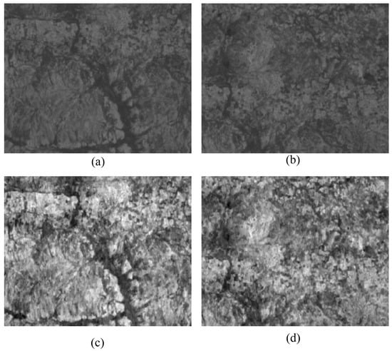
Figure 20. (a) The Nth frame noise image, (b) The N + 1th frame noise image, (c) the Nth frame of the image after processing by our method, (d) the N + 1th frame of the image after processing by our method.

In contrast algorithms, traditional statistical-based methods such as ADS and FPNE typically rely on assumptions that noise exhibits uniform statistical properties across the entire image. However, under the dynamic imaging conditions of low-orbit satellites, non-uniform noise exhibits strong spatial heterogeneity and temporal variability. Forcing global statistical estimation distorts structural information in real scenes, particularly in complex environments where large uniform areas (e.g., clouds, oceans) coexist with sharp edges (e.g., coastlines, urban outlines). This approach readily introduces blurring or generates new structured artifacts, degrading algorithm performance. Deep learning methods like FEU, SEID, ASCNET, and MDIVD are trained and modeled on highly regular periodic stripe noise. This noise exhibits high consistency between training and testing datasets, resulting in insufficient correction capabilities for diverse types of non-uniform noise.

6. Conclusions

In this work, we propose a tensor decomposition-based noise removal model for nonuniform noise using video image sequences. We employ a time-domain difference operator to constrain the sparsity of the noisy image and utilize one-way total variation regularization to enhance the Smoothness of the noisy image in the horizontal direction. Additionally, we apply $L_{2,1}$ regularization to improve the quality of the denoised image. We adopt an efficient ADMM algorithm to solve the proposed model. Experiments are conducted using simulated and actual data from the Qilu-2 satellite. Through a combination of qualitative and quantitative evaluations, the proposed method is found to outperform several state-of-the-art methods, demonstrating competitive performance and offering new insights for correcting nonuniformity in infrared video image sequences.

References

- Chen, J.; Shao, Y.; Guo, H.; Wang, W.; Zhu, B. Destriping CMODIS data by power filtering. IEEE Trans. Geosci. Remote Sens. 2003, 41, 2119–2124. [Google Scholar] [CrossRef]
- Lu, C. Stripe non-uniformity correction of infrared images using parameter estimation. Infrared Phys. Technol. 2020, 107, 103313. [Google Scholar] [CrossRef]
- Li, J.; Zeng, D.; Zhang, J.; Han, J.; Mei, T. Column-spatial correction network for remote sensing image destriping. Remote Sens. 2022, 14, 3376. [Google Scholar] [CrossRef]
- Zhou, D.; Wang, D.; Huo, L.; Liu, R.; Jia, P. Scene-based nonuniformity correction for airborne point target detection systems. Opt. Express 2017, 25, 14210–14226. [Google Scholar] [CrossRef] [PubMed]
- Liu, S.; Cui, H.; Li, J.; Yao, M.; Wang, S.; Wei, K. Low-contrast scene feature-based infrared nonuniformity correction method for airborne target detection. Infrared Phys. Technol. 2023, 133, 104799. [Google Scholar] [CrossRef]
- Liu, Y.; Qiu, B.; Tian, Y.; Cai, J.; Sui, X.; Chen, Q. Scene-based dual domain non-uniformity correction algorithm for stripe and optics-caused fixed pattern noise removal. Opt. Express 2024, 32, 16591–16610. [Google Scholar] [CrossRef] [PubMed]
- Liu, C.; Sui, X.; Liu, Y.; Kuang, X.; Gu, G.; Chen, Q. FPN estimation based nonuniformity correction for infrared imaging system. Infrared Phys. Technol. 2019, 96, 22–29. [Google Scholar] [CrossRef]
- Geng, L.; Chen, Q.; Qian, W. An adjacent differential statistics method for IRFPA nonuniformity correction. IEEE Photonics J. 2013, 5, 6801615. [Google Scholar] [CrossRef]
- Cao, Y.; Tisse, C.L. Shutterless solution for simultaneous focal plane array temperature estimation and nonuniformity correction in uncooled long-wave infrared camera. Appl. Opt. 2013, 52, 6266–6271. [Google Scholar] [CrossRef]
- Cao, C.; Dai, K.; Hong, S.; Zhang, M. Anisotropic total variation model for removing oblique stripe noise in remote sensing image. Optik 2021, 227, 165254. [Google Scholar] [CrossRef]
- Chang, Y.; Chen, M.; Yan, L.; Zhao, X.L.; Li, Y.; Zhong, S. Toward universal stripe removal via wavelet-based deep convolutional neural network. IEEE Trans. Geosci. Remote Sens. 2019, 58, 2880–2897. [Google Scholar] [CrossRef]
- Liu, L.; Zhang, T. Optics temperature-dependent nonuniformity correction via L0-regularized prior for airborne infrared imaging systems. IEEE Photonics J. 2016, 8, 3900810. [Google Scholar] [CrossRef]
- Wang, Y.; Wang, Y.; Liu, T.; Sui, X.; Gu, G.; Chen, Q. Enhancing infrared imaging systems with temperature-dependent nonuniformity correction via single-frame and inter-frame structural similarity. Appl. Opt. 2023, 62, 7075–7082. [Google Scholar] [CrossRef]
- Hou, E.S.H.; Li, J.; Kosonocky, W.F. Real-time implementation of two-point nonuniformity correction for IR-CCD imagery. In Proceedings of the SPIE—The International Society for Optical Engineering, San Diego, CA, USA, 9–14 July 1995; Volume 2598, pp. 44–50. [Google Scholar]
- Honghui, Z.; Haibo, L.; Xinrong, Y.; Qinghai, D. Adaptive non-uniformity correction algorithm based on multi-point correction. Infrared Laser Eng. 2014, 43, 3651–3654. [Google Scholar]
- Schulz, M.; Caldwell, L. Nonuniformity correction and correctability of infrared focal plane arrays. Infrared Phys. Technol. 1995, 36, 763–777. [Google Scholar] [CrossRef]
- Zhang, C.; Zhao, W. Scene-based nonuniformity correction using local constant statistics. JOSA A 2008, 25, 1444–1453. [Google Scholar] [CrossRef]
- Harris, J.G.; Chiang, Y.M. Nonuniformity correction of infrared image sequences using the constant-statistics constraint. IEEE Trans. Image Process. 1999, 8, 1148–1151. [Google Scholar] [CrossRef] [PubMed]
- Zuo, C.; Chen, Q.; Gu, G.; Sui, X.; Qian, W. Scene-based nonuniformity correction method using multiscale constant statistics. Opt. Eng. 2011, 50, 087006. [Google Scholar] [CrossRef]
- Zuo, C.; Zhang, Y.; Chen, Q.; Gu, G.; Qian, W.; Sui, X.; Ren, J. A two-frame approach for scene-based nonuniformity correction in array sensors. Infrared Phys. Technol. 2013, 60, 190–196. [Google Scholar] [CrossRef]
- Ratliff, B.M.; Hayat, M.M.; Hardie, R.C. Algebraic scene-based nonuniformity correction in focal plane arrays. In Proceedings of the SPIE—The Infrared Imaging Systems: Design, Analysis, Modeling, and Testing XII, Orlando, FL, USA, 10 September 2001; Volume 4372, pp. 114–124. [Google Scholar]
- Hardie, R.C.; Hayat, M.M.; Armstrong, E.; Yasuda, B. Scene-based nonuniformity correction with video sequences and registration. Appl. Opt. 2000, 39, 1241–1250. [Google Scholar] [CrossRef] [PubMed]
- Zuo, C.; Chen, Q.; Gu, G.; Sui, X. Scene-based nonuniformity correction algorithm based on interframe registration. J. Opt. Soc. Am. A 2011, 28, 1164–1176. [Google Scholar] [CrossRef]
- Zuo, C.; Chen, Q.; Gu, G.; Qian, W. New temporal high-pass filter nonuniformity correction based on bilateral filter. Opt. Rev. 2011, 18, 197–202. [Google Scholar] [CrossRef]
- Torres, S.N.; Hayat, M.M.; Armstrong, E.E.; Yasuda, B.J. Kalman-filtering approach for nonuniformity correction in focal plane array sensors. In Proceedings of the SPIE—The Infrared Imaging Systems: Design, Analysis, Modeling, and Testing XI, Orlando, FL, USA, 17 July 2000; Volume 4030, pp. 196–205. [Google Scholar]
- Torres, S.N.; Hayat, M.M. Kalman filtering for adaptive nonuniformity correction in infrared focal-plane arrays. J. Opt. Soc. Am. A 2003, 20, 470–480. [Google Scholar] [CrossRef]
- Liu, Z.; Ma, Y.; Fan, F.; Ma, J. Nonuniformity correction based on adaptive sparse representation using joint local and global constraints based learning rate. IEEE Access 2018, 6, 10822–10839. [Google Scholar] [CrossRef]
- Rossi, A.; Diani, M.; Corsini, G. Bilateral filter-based adaptive nonuniformity correction for infrared focal-plane array systems. Opt. Eng. 2010, 49, 057003. [Google Scholar] [CrossRef]
- Sheng-Hui, R.; Hui-Xin, Z.; Han-Lin, Q.; Rui, L.; Kun, Q. Guided filter and adaptive learning rate based non-uniformity correction algorithm for infrared focal plane array. Infrared Phys. Technol. 2016, 76, 691–697. [Google Scholar] [CrossRef]
- Lee, J.; Ro, Y.M. Dual-branch structured de-striping convolution network using parametric noise model. IEEE Access 2020, 8, 155519–155528. [Google Scholar] [CrossRef]
- Chang, Y.; Yan, L.; Liu, L.; Fang, H.; Zhong, S. Infrared aerothermal nonuniform correction via deep multiscale residual network. IEEE Geosci. Remote Sens. Lett. 2019, 16, 1120–1124. [Google Scholar] [CrossRef]
- Li, J.; Zhang, J.; Han, J.; Yan, C.; Zeng, D. Progressive recurrent neural network for multispectral remote sensing image destriping. IEEE Trans. Geosci. Remote Sens. 2023, 61, 1–18. [Google Scholar] [CrossRef]
- Wang, C.; Xu, M.; Jiang, Y.; Zhang, G.; Cui, H.; Li, L.; Li, D. Translution-SNet: A semisupervised hyperspectral image stripe noise removal based on transformer and CNN. IEEE Trans. Geosci. Remote Sens. 2022, 60, 5533114. [Google Scholar] [CrossRef]
- Zhang, D.; Zhou, F.; Jiang, Y.; Fu, Z. Mm-bsn: Self-supervised image denoising for real-world with multi-mask based on blind-spot network. In Proceedings of the IEEE/CVF Conference on Computer Vision and Pattern Recognition, Vancouver, BC, Canada, 17–24 June 2023; pp. 4189–4198. [Google Scholar]
- Wu, W.; Lv, G.; Liao, S.; Zhang, Y. FEUNet: A flexible and effective U-shaped network for image denoising. Signal Image Video Process. 2023, 17, 2545–2553. [Google Scholar] [CrossRef]
- Fang, H.; Wang, X.; Li, Z.; Wang, L.; Li, Q.; Chang, Y.; Yan, L. Detection-friendly nonuniformity correction: A union framework for infrared UAV target detection. In Proceedings of the Computer Vision and Pattern Recognition Conference, Nashville, TN, USA, 11–15 June 2025; pp. 11898–11907. [Google Scholar]
- Cao, B.; Wang, Q.; Zhu, P.; Hu, Q.; Ren, D.; Zuo, W.; Gao, X. Multi-view knowledge ensemble with frequency consistency for cross-domain face translation. IEEE Trans. Neural Netw. Learn. Syst. 2023, 35, 9728–9742. [Google Scholar] [CrossRef]
- Lin, X.; Li, Y.; Zhu, J.; Zeng, H. Deflickercyclegan: Learning to detect and remove flickers in a single image. IEEE Trans. Image Process. 2023, 32, 709–720. [Google Scholar] [CrossRef]
- Song, J.; Jeong, J.H.; Park, D.S.; Kim, H.H.; Seo, D.C.; Ye, J.C. Unsupervised denoising for satellite imagery using wavelet directional CycleGAN. IEEE Trans. Geosci. Remote Sens. 2020, 59, 6823–6839. [Google Scholar] [CrossRef]
- Shen, H.; Zhang, L. A MAP-based algorithm for destriping and inpainting of remotely sensed images. IEEE Trans. Geosci. Remote Sens. 2008, 47, 1492–1502. [Google Scholar] [CrossRef]
- Iordache, M.D.; Bioucas-Dias, J.M.; Plaza, A. Total variation spatial regularization for sparse hyperspectral unmixing. IEEE Trans. Geosci. Remote Sens. 2012, 50, 4484–4502. [Google Scholar] [CrossRef]
- Bouali, M.; Ladjal, S. Toward optimal destriping of MODIS data using a unidirectional variational model. IEEE Trans. Geosci. Remote Sens. 2011, 49, 2924–2935. [Google Scholar] [CrossRef]
- Chang, Y.; Fang, H.; Yan, L.; Liu, H. Robust destriping method with unidirectional total variation and framelet regularization. Opt. Express 2013, 21, 23307–23323. [Google Scholar] [CrossRef]
- Lu, X.; Wang, Y.; Yuan, Y. Graph-regularized low-rank representation for destriping of hyperspectral images. IEEE Trans. Geosci. Remote Sens. 2013, 51, 4009–4018. [Google Scholar] [CrossRef]
- Zhang, H.; He, W.; Zhang, L.; Shen, H.; Yuan, Q. Hyperspectral image restoration using low-rank matrix recovery. IEEE Trans. Geosci. Remote Sens. 2013, 52, 4729–4743. [Google Scholar] [CrossRef]
- Chang, Y.; Yan, L.; Chen, B.; Zhong, S.; Tian, Y. Hyperspectral image restoration: Where does the low-rank property exist. IEEE Trans. Geosci. Remote Sens. 2020, 59, 6869–6884. [Google Scholar] [CrossRef]
- Song, L.; Huang, H. Simultaneous destriping and image denoising using a nonparametric model with the EM algorithm. IEEE Trans. Image Process. 2023, 32, 1065–1077. [Google Scholar] [CrossRef]
- Zhang, J.; Zhou, X.; Li, L.; Hu, T.; Fansheng, C. A combined stripe noise removal and deblurring recovering method for thermal infrared remote sensing images. IEEE Trans. Geosci. Remote Sens. 2022, 60, 5003214. [Google Scholar] [CrossRef]
- He, Y.; Zhang, C.; Zhang, B.; Chen, Z. FSPnP: Plug-and-play frequency–spatial-domain hybrid denoiser for thermal infrared image. IEEE Trans. Geosci. Remote Sens. 2023, 62, 5000416. [Google Scholar] [CrossRef]
- Chang, Y.; Yan, L.; Wu, T.; Zhong, S. Remote sensing image stripe noise removal: From image decomposition perspective. IEEE Trans. Geosci. Remote Sens. 2016, 54, 7018–7031. [Google Scholar] [CrossRef]
- Wang, J.L.; Huang, T.Z.; Zhao, X.L.; Huang, J.; Ma, T.H.; Zheng, Y.B. Reweighted block sparsity regularization for remote sensing images destriping. IEEE J. Sel. Top. Appl. Earth Obs. Remote Sens. 2019, 12, 4951–4963. [Google Scholar] [CrossRef]
- Kolda, T.G.; Bader, B.W. Tensor decompositions and applications. SIAM Rev. 2009, 51, 455–500. [Google Scholar] [CrossRef]
- Cai, J.; He, W.; Zhang, H. Anisotropic spatial–spectral total variation regularized double low-rank approximation for HSI denoising and destriping. IEEE Trans. Geosci. Remote Sens. 2022, 60, 1–19. [Google Scholar] [CrossRef]
- Huitong, L.; Xinjian, Y. Two-point nonuniformity correction for IRFPA and its physical motivation. Infrared Laser Eng. 2004, 33, 76–78. [Google Scholar]
- Cao, W.; Wang, Y.; Sun, J.; Meng, D.; Yang, C.; Cichocki, A.; Xu, Z. Total variation regularized tensor RPCA for background subtraction from compressive measurements. IEEE Trans. Image Process. 2016, 25, 4075–4090. [Google Scholar] [CrossRef] [PubMed]
- Zhao, X.L.; Wang, F.; Ng, M.K. A new convex optimization model for multiplicative noise and blur removal. SIAM J. Imaging Sci. 2014, 7, 456–475. [Google Scholar] [CrossRef]
- Ding, S.; Wang, D.; Zhang, T. A median-ratio scene-based non-uniformity correction method for airborne infrared point target detection system. Sensors 2020, 20, 3273. [Google Scholar] [CrossRef]
- Zhuang, L.; Ng, M.K. FastHyMix: Fast and parameter-free hyperspectral image mixed noise removal. IEEE Trans. Neural Netw. Learn. Syst. 2021, 34, 4702–4716. [Google Scholar] [CrossRef]
- Cai, L.; Dong, X.; Zhou, K.; Cao, X. Exploring video denoising in thermal infrared imaging: Physics-inspired noise generator, dataset and model. IEEE Trans. Image Process. 2024, 33, 3839–3854. [Google Scholar] [CrossRef]
- Yuan, S.; Qin, H.; Yan, X.; Yang, S.; Yang, S.; Akhtar, N.; Zhou, H. ASCNet: Asymmetric sampling correction network for infrared image destriping. IEEE Trans. Geosci. Remote Sens. 2025, 63, 5001815. [Google Scholar] [CrossRef]
- Ying, X.; Liu, L.; Lin, Z.; Shi, Y.; Wang, Y.; Li, R.; Cao, X.; Li, B.; Zhou, S.; An, W. Infrared small target detection in satellite videos: A new dataset and a novel recurrent feature refinement framework. IEEE Trans. Geosci. Remote Sens. 2025, 63, 5002818. [Google Scholar] [CrossRef]
- Wang, Z.; Bovik, A.C.; Sheikh, H.R.; Simoncelli, E.P. Image quality assessment: From error visibility to structural similarity. IEEE Trans. Image Process. 2004, 13, 600–612. [Google Scholar] [CrossRef]
- Hore, A.; Ziou, D. Image quality metrics: PSNR vs. SSIM. In Proceedings of the 2010 20th International Conference on Pattern Recognition, Istanbul, Turkey, 23–26 August 2010; IEEE: Piscataway, NJ, USA, 2010; pp. 2366–2369. [Google Scholar]
- Huynh-Thu, Q.; Ghanbari, M. Scope of validity of PSNR in image/video quality assessment. Electron. Lett. 2008, 44, 800–801. [Google Scholar] [CrossRef]
- Li, L.; Song, S.; Lv, M.; Jia, Z.; Ma, H. Multi-Focus Image Fusion Based on Fractal Dimension and Parameter Adaptive Unit-Linking Dual-Channel PCNN in Curvelet Transform Domain. Fractal Fract. 2025, 9, 157. [Google Scholar] [CrossRef]
- Li, F.; Rao, P.; Sun, W.; Su, Y.; Chen, X. A new motion feature-enhanced multiframe spatial–temporal infrared target detection network. IEEE Trans. Geosci. Remote Sens. 2025, 63, 5006819. [Google Scholar] [CrossRef]
- Li, S.; Yang, Z.; Li, H. Statistical evaluation of no-reference image quality assessment metrics for remote sensing images. ISPRS Int. J. Geo-Inf. 2017, 6, 133. [Google Scholar] [CrossRef]
- Mittal, A.; Soundararajan, R.; Bovik, A.C. Making a “completely blind” image quality analyzer. IEEE Signal Process. Lett. 2012, 20, 209–212. [Google Scholar] [CrossRef]
Disclaimer/Publisher’s Note: The statements, opinions and data contained in all publications are solely those of the individual author(s) and contributor(s) and not of MDPI and/or the editor(s). MDPI and/or the editor(s) disclaim responsibility for any injury to people or property resulting from any ideas, methods, instructions or products referred to in the content. |
© 2025 by the authors. Licensee MDPI, Basel, Switzerland. This article is an open access article distributed under the terms and conditions of the Creative Commons Attribution (CC BY) license.