Highlights
What are the main findings?
- This study proposes a Global-Local enhanced Deformable Convolution Network (GLDCN), which achieves efficient long-range semantic modeling through a dynamic offset mechanism.
- The designed Adaptive Channel Attention Module (ACAM) effectively addresses the cross-modal fusion challenge between optical and SAR data through an adaptive weighting mechanism, thereby reducing misclassification among easily confusable categories.
What are the implications of the main findings?
- The GLDCN balances computational efficiency and modeling capability, significantly enhancing the extraction of features such as sea ice edges and textures.
- ACAM demonstrates the effectiveness of the multimodal fusion strategy, which not only substantially improves sea ice classification accuracy but also exhibits robust generalization capability.
Abstract
As a critical indicator of polar ecosystem dynamics, sea ice monitoring plays a pivotal role in climate change. However, as global warming accelerates the melting of sea ice, the complexity in the Arctic poses growing challenges for achieving high-precision sea ice classification. To address this issue, this study begins with the creation of a multi-source sea ice dataset based on GaoFen-3 fully polarimetric SAR data and Landsat optical imagery. In addition, the study proposes a Global–Local enhanced Deformable Convolution Network (GLDCN), which effectively captures long-range semantic dependencies and fine-grained local features of sea ice. To further enhance feature integration, an Adaptive Channel Attention Module (ACAM) is designed to achieve adaptive weighted fusion of heterogeneous SAR and optical features, substantially improving the model’s discriminative ability in complex conditions. Experimental results show that the proposed method outperforms several mainstream models on multiple evaluation metrics. The multi-source data fusion strategy significantly reduces misclassification among confusable categories, validating the importance of multimodal fusion in sea ice classification.
1. Introduction
Sea ice is an essential component of the Earth’s cryosphere and plays a central role in the global climate system. Its high albedo, low thermal conductivity, and ability to modulate oceanic thermohaline circulation profoundly influence global energy balance and material cycling processes. With global warming, sea ice in the Arctic and globally is undergoing unprecedented rapid changes, characterized by a continuous decline in areal extent and a marked trend toward a younger ice age structure [1,2]. Against this background, the accurate identification of sea ice types and continuous monitoring of their spatiotemporal dynamics have become a critical scientific task, which is vital for understanding climate feedback mechanisms, ensuring polar navigation safety, and sustaining the stability of ice ecosystems [3].
With the rapid advancement of remote sensing technology, the use of remote sensing imagery for sea ice classification has become a mainstream methodology. Current primary monitoring techniques include passive microwave radiometers, optical sensors, and SAR. Passive microwave radiometers primarily distinguish sea ice from open water based on their significant differences in radiative properties, offering extensive spatial coverage but with limited spatial resolution, which restricts their capability for detailed classification. Optical sensors can provide high-resolution and intuitive information, enabling accurate classification of sea ice. However, their observations are heavily dependent on illumination conditions and are susceptible to interference from clouds and fog. SAR exhibits notable advantages in sea ice monitoring due to its high spatial resolution and all-weather, day-and-night imaging capability. Most existing studies rely on single-polarization SAR data for terrain identification. However, single-polarization data have inherent limitations in characterizing sea ice texture features, making accurate classification challenging. In contrast, fully polarimetric SAR can acquire data in four polarization channels (HH, HV, VH, and VV), and the diverse scattering mechanisms provide richer feature information, thereby enabling more precise sea ice classification and scene interpretation [4,5]. Nevertheless, affected by its coherent imaging mechanism, SAR imagery is subject to speckle noise, which substantially degrades image quality and interpretation accuracy. Moreover, SAR imagery captures the microwave backscattering intensity from surface targets rather than intuitive brightness information, which makes its interpretation more difficult than that of optical imagery.
Given the distinct advantages and limitations of the aforementioned sensors, a single data source proves insufficient for comprehensively characterizing sea ice, making it difficult to achieve highly accurate and reliable sea ice classification. Consequently, fusing multi-source remote sensing data to leverage their complementary information has emerged as a crucial pathway for enhancing both the classification accuracy and model robustness. Li et al. [6] achieved pixel-level fusion of Sentinel-1 SAR and Sentinel-2 optical data by solving the Poisson equation, significantly enhancing spatial details and texture representation. Zhao et al. [7] integrated Sentinel-1 SAR imagery with AMSR-2 data, enabling efficient and precise classification of sea ice across entire scenes. Their experiments demonstrated that this approach significantly outperforms traditional methods and single-source fusion techniques. Wiehle et al. [8] utilized SAR data from Sentinel-1 and optothermal data from Sentinel-3 to discriminate among six sea ice types. Compared with classification using SAR data alone, the combined method resulted in improved classification reliability. Wu et al. [9] proposed a multi-task sea ice inversion method that fuses SAR and AMSR-2 data to simultaneously predict sea ice concentration, stage of development, and floe size. However, their fusion strategy relied on simple concatenation, which might lead to information loss. Existing methods face challenges such as limited registration accuracy and inefficient interaction of heterogeneous information, underscoring the urgent need to develop novel fusion algorithms to achieve a significant leap in sea ice classification accuracy.
In recent years, the remarkable success of deep learning in image classification has rapidly extended to sea ice classification research, gradually replacing traditional machine learning methods. Compared with machine learning approaches, deep learning can automatically learn multi-level, high-dimensional feature representations from raw remote sensing data without relying on expert-driven feature engineering. Within this context, various advanced deep learning models have been widely applied to sea ice classification, such as Convolutional Neural Networks (CNNs) and Transformers. Boulze et al. [10] proposed a CNN framework for SAR-based sea ice classification, achieving fine-grained discrimination among four target classes: Open Water, Young Ice, First-Year Ice, and Multi-Year Ice. Compared with traditional machine learning paradigms such as Random Forest, this CNN model significantly improved classification accuracy. Xu et al. [11] further introduced a transfer learning mechanism, using AlexNet as the backbone to extract deep features from image patches, attaining the accuracy of on the test set. Zhang et al. [12] adopted MobileNetV3 as the baseline and constructed a multi-scale feature fusion framework, effectively enhancing the sea ice classification performance for GaoFen-3 imagery. Zhao et al. [13] embedded VGG-16 and ResNet-50 into the encoder of U-Net, proposing two improved architectures named VU-Net and RU-Net, respectively, and validated their effectiveness on a mid-to-high-latitude winter sea ice dataset acquired by aerial cameras. Ren et al. [14] proposed a U-Net–based model for classifying ice and water in SAR imagery, enabling pixel-level sea-ice classification. Subsequently, by incorporating a dual-attention mechanism, the authors developed an enhanced U-Net model that achieved higher segmentation accuracy than the original model [15]. Zhang et al. [16] proposed SI-CTFNet for GaoFen-3 SAR data, which integrates a dual-branch CNN-Transformer architecture and a cross-modal feature fusion module, significantly enhancing discriminative capability in complex scenarios. However, while CNNs excel in computational efficiency, they cannot capture long-range semantic dependencies. In contrast, Vision Transformer (ViT) can effectively model global contextual information, but its high computational complexity leads to significant time and memory overhead.
To address these challenges, this paper builds a high-quality sea ice classification dataset based on SAR and optical data, and proposes two methods: GLDCN and ACAM. The GLDCN backbone effectively models long-range semantic dependencies while maintaining linear computational complexity. The fusion module ACAM is designed to achieve adaptive fusion of heterogeneous features, significantly improving the accuracy of sea ice classification. The main contributions of this work are summarized as follows:
(1) This study systematically collects GaoFen-3 fully polarimetric SAR data and Landsat-series optical imagery. Then we employ a spatiotemporal correlation-based image matching algorithm to screen for well-matched image pairs in both space and time, and construct a multi-source sea ice dataset. The dataset consists of 2664 samples spanning four typical sea ice categories: Open Water (OW), New Ice (NI), Young Ice (YI), and Multi-Year Ice (MYI), which provides a high-quality data basis for subsequent deep learning modeling.
(2) We propose a novel backbone network, GLDCN, which aims to achieve both long-range semantic modeling and computational efficiency. By incorporating a dynamic offset mechanism, the model achieves adaptive receptive field adjustment and long-range information modeling with linear computational complexity, thereby significantly enhancing its capability to extract discriminative features such as sea ice edges and textures.
(3) To address the challenge of fusing heterogeneous optical and SAR data, this paper proposes the ACAM for effective cross-modal feature fusion. Through a channel-wise weighting mechanism, ACAM enables the model to autonomously prioritize either optical or SAR dominant features based on the actual scene. This facilitates robust fusion in complex conditions, thereby significantly improving the distinction between easily confused sea ice types.
The remainder of this paper is organized as follows. Section 2 describes the construction of the dataset. Section 3 elaborates on the proposed backbone network and fusion module. Experiments and an analysis of the proposed model’s performance are presented in Section 4. Finally, Section 5 draws the conclusions of the study.
2. Geographical Scope and Dataset
In current remote sensing technology, passive microwave radiometers, optical sensors and SAR serve as the primary means for acquiring terrestrial information. Nevertheless, the relatively low spatial resolution of passive microwave radiometers somewhat limits their capability to observe detailed surface features. Consequently, we explore the fusion of SAR and optical data to enhance dataset quality and usability. A temporal correlation-based matching algorithm for remote sensing images is developed. This algorithm automatically identifies image pairs with acquisition time intervals within 24 h from globally collected optical and SAR satellite imagery. Subsequently, manual visual inspection is applied to exclude pairs exhibiting excessive geolocation discrepancies in the target areas. Following this procedure, the Sea of Okhotsk in late winter and early spring is selected as the primary study area, with data sourced from the GaoFen-3 satellite and the Landsat series. The study area is presented in Figure 1.
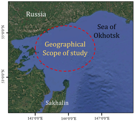
Figure 1.
The study region of the Sea of Okhotsk.
2.1. The Sea of Okhotsk
Located in the northwest Pacific, the Sea of Okhotsk spans approximately 1.583 million square kilometers. It possesses a largely straight coastline, measuring about 10,460 km in total length and indented by major bays. As a crucial conduit for heat and moisture exchange between continental East Asia and the North Pacific, sea ice dynamic here plays a significant role in regulating atmospheric circulation patterns and the climate of East Asia. During the late winter and early spring, the sea ice cover undergoes rapid diminution in both area and thickness. The ensuing interaction between water and ice generates a highly complex maritime scenario characterized by a wide variety of ice types. Consequently, the area is highly recommended for sea ice classification research.
2.2. GaoFen-3 SAR Data
Launched in 2016, the GaoFen-3 satellite is China’s first SAR satellite operating in the C-band with multi-polarization capabilities, providing imagery at a resolution of one meter. It also boasts the most imaging modes of any spaceborne SAR system to date. This radar system supports full-polarization transmission and reception and covers 12 imaging modes, including stripmap, spotlight, scanSAR, wave, and so on, with spatial resolutions ranging from 1 m to 500 m and swath widths from 10 km to 650 km. Full-polarization data contain four polarization channels, the scattering mechanisms of which comprehensively capture the textural characteristics of sea ice. Thus, we utilize the satellite’s full-polarization stripmap 1 mode, which provides an imagery resolution of approximately 8 m.
2.3. Landsat Optical Data
The Landsat program represents the world’s longest-running civilian Earth observation system, maintaining the most complete historical archive, and is jointly managed by NASA and the USGS. Up to now, nine satellites have been successfully launched. This study utilizes optical remote sensing data acquired from Landsat-8 and Landsat-9, which were launched in 2013 and 2021. Both satellites offer 11 spectral bands with spatial resolutions of 15 or 30 m, thereby providing detailed surface information. Among these 11 bands, the red, green, and blue bands are selected. As different ground objects possess distinct material compositions and surface states, they exhibit unique spectral response characteristics. True-color composites generated from these three bands directly map these spectral differences into color variations, allowing for more intuitive discrimination of various features and effectively enhancing the accuracy and efficiency of image interpretation.
2.4. The Extraction of Polarimetric Information from SAR Data
Fully polarimetric SAR data contain rich polarimetric information, for which we perform polarimetric feature extraction. The scattering matrix S is constructed from HH, HV, VH, and VV polarizations, as shown in Equation (1). Due to the reciprocity theorem, the scattering matrix satisfies , and thus only HH, HV, and VV polarizations are utilized here. Subsequently, we calculate the polarization ratios and coherence parameter (PRCD) and the polarimetric decomposition parameter (PDP) from the fully polarimetric SAR data.
(1) PRCP
Seven PRCPs are extracted from the scattering matrix S, including the total power (), the co-polarization ratios (), the cross-polarization ratios (, ), the depolarization correlation coefficient (), the polarization difference (), and the co-polarization phase difference ().
where Re and Im are the real and imaginary parts of the complex number, denotes the conjugate transpose of matrix x, and is the amplitude of the complex number.
The seven PRCDs establish an integrated analytical framework for characterizing sea ice types and their physical properties. The total power represents the overall scattering intensity of sea ice. The co-polarization and cross-polarization ratios serve as effective indicators of surface roughness. The polarization difference and depolarization correlation coefficient reflect the complexity of the internal structure. The co-polarization phase difference aids in identifying the dominant scattering mechanism. Together, these parameters systematically characterize the electromagnetic scattering behavior of sea ice from multiple dimensions, providing a comprehensive physical basis for high-accuracy sea ice classification.
(2) PDP
Polarimetric decomposition utilizes the scattering characteristics of polarimetric SAR data across different polarization channels to enable comprehensive analysis and feature extraction of target physical properties, such as orientation, shape, and material composition. Subsequently, PDPs are derived from the scattering matrix. For PDPs’ extraction, we employ the mathematically principled Cloude–Pottier decomposition [17] and the physics-based Freeman–Durden decomposition [18].
The Cloude–Pottier decomposition, also referred to as the H/A/ decomposition, is a prominent method in polarimetric SAR processing. This method is based on the eigen-decomposition of the coherency matrix derived from polarimetric SAR data. Computing the eigenvalues and eigenvectors of the coherency matrix facilitates the retrieval of the target’s polarimetric properties. First, the Pauli vector is derived from the scattering matrix and defined as follows:
The product of and its conjugate transpose yields a second-order matrix known as the polarimetric coherence matrix [T], which takes the following form:
The covariance matrix is decomposed into its eigenvectors and eigenvalues, which takes the following form:
where are eigenvalues and [U] is the unitary matrix, whose columns correspond to the orthogonal eigenvectors of [T]. Three PDPs: the entropy (H), anisotropy (A) and alpha-angle () can be derived from the eigenvalues.
where . The scattering entropy H () characterizes the degree of randomness of scatterers. When H = 0, the target is fully polarized and the scattering process is deterministic. When H = 1, the scattering process degenerates into completely random noise, and no effective polarimetric information of the target can be obtained. The anisotropy A (), serving as a complement to scattering entropy, describes the relative relationship between the two secondary scattering mechanisms. In general, when , A can provide additional polarimetric information to complement the scattering entropy. The scattering angle primarily describes the intrinsic degrees of freedom of the target, with values ranging between 0° and 90°, and mainly represents the shape and structure of the scatterer. When °, the target is an isotropic surface, corresponding to odd-bounce scattering. As increases, the target becomes an anisotropic surface; at °, it represents a dipole; when °, it corresponds to an anisotropic dihedral structure, associated with even-bounce scattering and at °, it denotes an isotropic dihedral reflector [19].
Subsequently, the Freeman–Durden decomposition is performed. This decomposition provides a simple and practical approach for polarimetric SAR decomposition studies. Based on a physical model, it proposes three scattering mechanisms: (1) first-order Bragg surface scattering, (2) double-bounce scattering from dihedral corner reflectors, (3) canopy scattering from randomly oriented dipoles. Accordingly, ground object scattering is categorized into surface scattering, double-bounce scattering, and volume scattering. The power of these three scattering components can be extracted from the polarimetric covariance matrix [T].
where , , and represent the coefficients for surface scattering, double-bounce scattering, and volume scattering, respectively, while , , and denote the corresponding scattering models. Equation (16) represents the backscattering model derived from Equation (15), where the parameter indicates the ratio of vertical-to-horizontal backscattering in double-bounce scattering, and denotes the surface Bragg scattering coefficient. During the solution of Equation (16), it is observed that there are four equations but five unknowns, necessitating assumptions for the values of and based on contextual considerations. If is positive, surface scattering is determined to be dominant, and is set to −1 accordingly. Conversely, if is negative, double-bounce scattering is identified as dominant, and is set to 1 accordingly [18]. After solving, we obtain the three scattering powers , , and , as shown in Equation (17).
The three components derived from the Freeman–Durden decomposition effectively characterize different sea ice types, thereby significantly contributing to sea ice segmentation. For smooth surfaces such as open water, surface scattering is dominant. In the case of ice ridges, where reflections occur between two orthogonal surfaces, double-bounce scattering prevails. For heavily deformed ice or the layered structure of multi-year ice, multiple reflections lead to volume scattering dominance [19].
The polarimetric decomposition feature maps obtained from both Cloude–Pottier and Freeman–Durden decompositions are visualized and compared with the amplitude of the original polarimetric data, as shown in Figure 2. During the extraction of polarimetric features, a total of 13 features are derived, including 7 PRCPs and 6 PDPs.
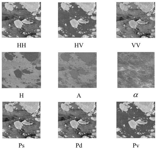
Figure 2.
Original polarization data and polarization decomposition feature maps.
2.5. Multi-Source Remote Sensing Dataset
The dataset construction workflow is illustrated in Figure 3. For the SAR data processing, preprocessing steps are sequentially performed, including geometric correction, noise reduction, polarimetric information extraction, and histogram equalization. For the optical data, the procedures involve geometric calibration, atmospheric correction, noise reduction and pixel value normalization. In the denoising step, a modified 3 × 3 Lee filter [20] is uniformly applied across both data types. This filter effectively suppresses noise and preserves image detail. Following preprocessing, the SAR data comprises 16 channels, including the amplitude components of the HH, HV, and VV polarizations along with 13 derived polarimetric features. The optical data consist of the three visible bands: red, green, and blue.
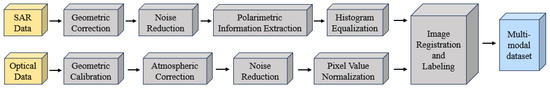
Figure 3.
Multi-source dataset construction workflow.
Subsequently, the SAR data are downsampled using the Lanczos algorithm [21] to match the spatial resolution of the optical data. This process effectively suppresses inherent speckle noise and preserves these decisive macroscopic spatial structures and contextual features. On this basis, pixel-level precise registration is conducted between the SAR and optical images to ensure strict spatial-geometric alignment, providing a reliable foundation for subsequent fusion. The images are then uniformly cropped into patches of 224 × 224 pixels, yielding a total of 2664 samples. These samples are split into train and test sets in a 7:3 ratio for model training and testing, respectively.
Finally, with reference to the criteria specified by the World Meteorological Organization (WMO), sea ice is categorized into four distinct classes: OW, NI, YI and MYI. Ground truth labels are generated via a hybrid strategy integrating “USNIC ice chart macro-guidance + optical image collaborative manual annotation”. The ice charts released by the USNIC provide large-scale distribution information on sea ice types, which serve as an initial reference for establishing the overall classification framework and spatial distribution patterns. Building upon this foundation, collaborative manual annotation is conducted using high-resolution optical images. In Landsat optical imagery, the four sea ice types exhibit distinct visual characteristics owing to variations in thickness and surface reflectance. Specifically, OW presents a black appearance, NI appears dark gray, YI shows a grayish-white hue, and MYI typically displays a bright white color. The outcomes of data matching and annotation are presented in Figure 4 and Figure 5.
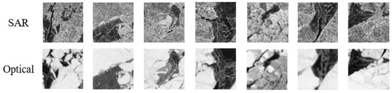
Figure 4.
Matching results of SAR and optical images.
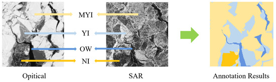
Figure 5.
Annotated schematic diagram.
3. Method
The overall architecture of the proposed model is illustrated in Figure 6, which consists of three components: a backbone network named GLDCN for feature extraction, a fusion module termed ACAM for effective information interaction, and a decoder for restoring the original spatial resolution. Specifically, optical and SAR data are fed into two separate branches, both employing GLDCN as the backbone network to extract multi-scale sea ice features. Subsequently, the features extracted at each layer undergo fusion in the ACAM module, which adaptively selects appropriate channels to achieve efficient fusion and deep integration of information. Finally, the fused features are processed by the decoder to generate the output.
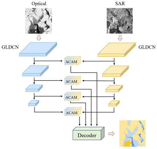
Figure 6.
Model framework diagram.
3.1. Backbone
The proposed backbone network, GLDCN, is illustrated in Figure 7. This network adopts a four-stage progressive architecture, where each stage primarily consists of a lightweight Global-Local Extraction Module (GLEM) and a Deformable Convolutional Network Module (DCNM). By introducing a complementary mechanism for global and local features and leveraging dynamic convolution to facilitate information interaction across different sea ice sampling points, GLDCN effectively models long-range spatial dependencies within sea ice imagery. This design helps mitigate the limitations of traditional CNNs in capturing discriminative features such as sea ice edges and textures.
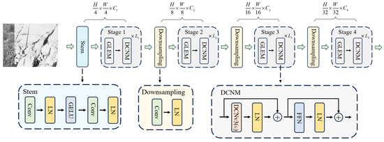
Figure 7.
Architecture of GLDCN.
For an input image of spatial size H × W, the computational complexity of DCNM with input and output channels of and , is , scaling linearly with the total number of image pixels. In contrast, the computational complexity of ViT with an embedding dimension of L is dominated by a term that scales quadratically with the total number of pixels, resulting in an overall complexity of . Consequently, when processing high-resolution remote sensing images of sea ice, the proposed network exhibits superior computational and memory efficiency, making it more suitable for deployment in practical applications.
3.1.1. Basic Block
The core of the basic block consists of two components: GLEM and DCNM. The GLEM adopts a global-local complementary mechanism to perform preliminary extraction and feature enhancement on the input information at each stage. Building upon this, the DCNM constructs long-range semantic dependencies, enabling multi-level deep learning of data features.
As illustrated in Figure 8, the GLEM captures global distributions and local details through a dual-branch structure. In the Global Enhancement (GE) branch, global average pooling (GAP) is applied to the input features, producing channel-wise statistics that characterize large-scale sea ice information. The Local Enhancement (LE) branch reshapes the input tensor into a 1 × 1 × (C × H × W) representation and utilizes 1 × 1 convolution to capture pixel-level contextual relationships while preserving spatial resolution. Following feature extraction in each branch, the resulting representations are restored to their original spatial dimensions via Up-sampling and combined through element-wise summation. This integration yields hybrid attention weights that effectively balance global consistency with local discriminability. Finally, these weights are applied to the original features, achieving lightweight enhancement with channel-spatial coupling.
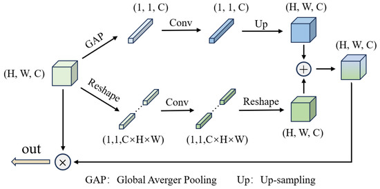
Figure 8.
Architecture of GLEM.
As is well recognized, sea ice exhibits considerable variation in size. The GE branch within the GLEM framework provides global contextual information, which contributes to capturing the overall size of sea ice. Moreover, certain sea ice formations are characterized by fragmented patterns and complex boundary structures. The LE branch in GLEM incorporates local spatial context, effectively enhancing discriminative feature representation at the interface between thin ice and open water. By leveraging the complementary nature of global and local information, the GLEM module achieves stability enhancement and preliminary feature extraction of sea ice data, thereby establishing a robust feature foundation for downstream core processing modules.
The DCNM is structured around several components: the DCNv3 operator [22], Layer Normalization (LN) [23] and Feed-Forward Networks (FFN) [24]. In the DCNM, the input data undergoes a series of operations—DCNv3, LN, and a residual connection. Then, the resulting features pass through FFN and LN, ultimately concluding with the second residual connection. This architectural design has been demonstrated to be effective in numerous visual tasks [25,26].
The principle of DCNM is built upon the DCNv3 operator, which enables dynamic, sparse, and adaptive feature sampling. Specifically, through a grouping operation, DCNv3 predicts a spatial offset and an importance modulation scalar for every sampling point k, based on a given central point on the input feature map within each group. This deformable convolution process can be mathematically expressed as follows:
In this process, the offset dynamically adjusts the sampling positions based on the input, thereby breaking the constraints of fixed geometric structures and enabling dependency modeling from short-range to long-range. This mechanism enables each branch of the network to slightly adjust sampling positions to correct minor geometric misalignments between SAR and optical images caused by sea ice drift. The modulation scalars , function similarly to attention weights, adaptively emphasizing or suppressing the feature contributions from different sea ice sampling points. Furthermore, DCNv3 incorporates two key designs to enhance its feasibility as a core component of foundational models. First, the weight sharing, where all convolutional neurons within the same group share the same set of convolution weights, significantly reduces parameter count and memory consumption. Second, the multi-group mechanism allows each group to independently learn its own offsets and modulation scalars, enabling the model to capture diverse contextual information in parallel from the input features, which enhances its expressive capacity and feature hierarchy.
3.1.2. Stem and Downsampling Layers
Multi-scale feature fusion is a widely adopted strategy in the field of semantic segmentation. Its idea lies in the cascade capture of hierarchical representations, ranging from local details to global semantics. Shallow features, characterized by high spatial resolution, are capable of precisely delineating fine-grained information such as edges and textures. In contrast, deeper features possess a broader receptive field, enabling the modeling of large-scale structures and contextual dependencies. In our architecture, stem and downsampling layers are used to adjust the feature maps to different scales, with the detailed structure illustrated in Figure 7. The stem layer, positioned prior to the first stage, reduces the input resolution by a factor of four for preliminary feature extraction. It consists of convolutional layers (kernel size: 3 × 3, stride: 2, padding: 1), LN and GELU activation. The downsampling layer, composed of a convolution layer (kernel size: 3 × 3, stride: 2, padding: 1) and LN, is placed between two consecutive Basic Block stages.
3.2. Fusion
In the specialized remote sensing task of sea ice classification, effectively fusing optical and SAR data represents a vital challenge in enhancing model performance. Optical imagery, dependent on reflected light, delivers rich spectral information that is crucial for distinguishing various ice surface characteristics, yet it is significantly influenced by illumination and weather conditions. Conversely, SAR imagery, based on microwave backscatter, is sensitive to the surface roughness and physical structure of sea ice and provides all-weather, day-and-night observation capability, but it is inherently susceptible to speckle noise. The relative importance of these two data sources varies dynamically across different sea ice types and environmental conditions. Simple feature concatenation or linear fusion approaches are often inadequate in handling such complexity, potentially resulting in information loss or noise introduction. To overcome these limitations, this paper introduces an ACAM, as depicted in Figure 9. This module implements a dynamic selection mechanism that allows the network to adaptively recalibrate the significance of optical and SAR features based on the input context, thereby enabling more intelligent and robust feature fusion.
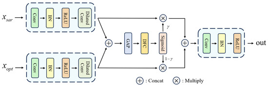
Figure 9.
Architecture of ACAM.
The module first performs preprocessing on the features extracted from the backbone network. Specifically, the SAR features and optical features output by the backbone are processed separately by two independent structural branches. Each branch sequentially consists of a 3 × 3 convolutional layer, a Batch Normalization (BN) layer, a ReLU activation function, and a dilated convolutional layer. The dilated convolutional layer (dilation rate = 3) serves to expand the receptive field, thereby capturing more representative contextual information. This design employs separate branches for feature extraction from SAR and optical data prior to fusion, which mitigates potential information loss caused by data heterogeneity. This preprocessing pipeline establishes a robust foundation for subsequent deep fusion, effectively bridging the potential semantic gap arising from different data modalities.
The preprocessed features are first concatenated to form a foundational joint representation. This representation is compressed by GAP into a global channel-wise descriptor, which is then transformed through two fully-connected layers and a sigmoid activation to produce an adaptive channel-weight vector . Acting as a channel-confidence gating mechanism, encodes the relative importance of SAR and optical data across feature channels. During fusion, the vector and its complement (1 – ) are applied to the weight of the preprocessed optical and SAR features, respectively, establishing an adaptive “select-and-emphasize” mechanism. For example, in sea ice scenes affected by significant SAR speckle noise, the network learns to assign lower values in , thereby suppressing noisy SAR features and emphasizing optical information. Conversely, under cloud cover or during nighttime imaging conditions, the network elevates the weights in the corresponding channels of , directing the fused output to rely predominantly on SAR-derived textural features. This effectively circumvents interference from unreliable optical information.
This dynamic, context-sensitive modulation capability allows the model to adapt to varying meteorological and illumination conditions, significantly improving the robustness and practical applicability of the sea ice classification system. The weighted optical and SAR features are then concatenated and passed through a 1 × 1 convolution, BN, and ReLU activation for dimensionality reduction and feature integration, outputting a refined fused representation. The entire process is formalized in Equations (19)–(22).
In summary, the proposed module embeds dynamic channel attention into multi-source remote sensing fusion. Instead of treating optical and SAR inputs as static and equally weighted, it enables the network to adaptively recalibrate their contributions according to scene content. This approach enhances discriminative ability and generalization in challenging scenarios, offering a reliable technical pathway toward operational high-precision sea ice classification.
3.3. Decoder
The decoder component, inspired by the cascade strategy of UPerHead [27], proposes a cooperative upsampling fusion mechanism designed to fully exploit and restore multi-scale fused features, as illustrated in Figure 10. For details, starting from the multi-level features F1, F2, F3, and F4 output by the fusion layer, the decoder progressively performs semantic enhancement and spatial resolution alignment. First, the features from all four levels are upsampled via bilinear interpolation to restore the spatial resolution of the initial input. Subsequently, a 3 × 3 convolution layer, BN layer, and ReLU activation are independently applied to each feature layer to refine local details and transform channel-wise semantics. Then, four feature layers are concatenated along the channel dimension to construct a fused representation. Finally, a 1 × 1 convolution is employed for channel compression and pixel-wise segmentation prediction, producing segmentation results that effectively preserve fine-grained structures. By aggregating semantic information from various network levels, the proposed decoder achieves deep utilization of features, significantly enhancing the model’s ability to interpret complex sea ice conditions.
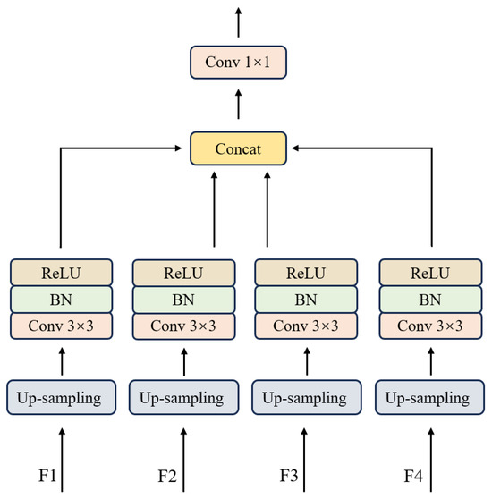
Figure 10.
Structure of the decoder.
4. Experimental Results
The experimental design and analysis are organized into four sections. Section 4.1 introduces the evaluation metrics employed in this study. Section 4.2 presents comparative experiments using different backbone networks, in which SAR and optical data are concatenated along the channel dimension to form a 19-channel input, allowing for a systematic assessment of various backbone architectures. Section 4.3 focuses on the comparative analysis of fusion modules, where 16-channel SAR data and 3-channel optical data are processed through independent encoding branches and subsequently integrated using different fusion strategies. Section 4.4 describes the data-level ablation experiments conducted to systematically verify the effectiveness of polarimetric features and to demonstrate the complementary characteristics and fusion advantages of heterogeneous remote sensing data.
4.1. Evaluation Metrics System
To comprehensively evaluate the semantic segmentation performance of the proposed model, four key metrics were employed: Pixel Accuracy (PA), Class Pixel Accuracy (CPA), Mean Intersection over Union (mIoU), and the Kappa coefficient. PA quantifies the overall proportion of correctly classified pixels across all categories, while CPA measures this proportion for each category. These metrics serve as key indicators for evaluating the model’s pixel-level performance. However, relying solely on these metrics may be misleading in datasets with class imbalance, as it fails to accurately reflect the model’s ability to segment minority classes. IoU calculates the ratio between the intersection and the union of the predicted and ground-truth regions. It penalizes both false positives and false negatives, thereby providing a precise evaluation of the model’s capability in segmenting object shapes and boundaries. mIoU is obtained by averaging the IoU values across all classes. Furthermore, to assess the agreement between the model’s predictions and the ground-truth annotations while accounting for the effects of random chance, the Kappa coefficient is also adopted. This metric is particularly reliable in evaluating models under class-imbalanced conditions. Collectively, these metrics provide a comprehensive and rigorous assessment of the model’s performance from multiple perspectives.
- : True Positives for the n-th class
- : True Negatives for the n-th class
- : False Positives for the n-th class
- : False Negatives for the n-th class
- N: Number of categories
4.2. Comparison of Methods
In the sea ice classification task, this study systematically evaluates the performance of the proposed GLDCN method and conducts comparative analyses with several classical semantic segmentation models, including CNN-based architectures such as FCN [28], DeepLabv3+ [29], PSPNet [30], U2Net [31], MobileNetV3 [32], InternImage [22], and ViT-based models such as Swin [26], PVT [33], BEiT2 [34]. The experimental results presented in Table 1 demonstrate that the proposed GLDCN method achieves the best performance across multiple evaluation metrics, with PA, mIoU, and Kappa coefficient reaching 94.81%, 88.94%, and 92.21%, respectively. Moreover, GLDCN maintains superior classification performance across the three ice categories: YI, NI, and MYI, exhibiting remarkable classification capability.

Table 1.
Performance comparison of models.
From Table 1, it is observed that FCN, Deeplabv3+, PSPNet, and MobileNetV3 exhibit subpar performance, with PA values clustering in the 84–88% range, mIoU approximately 70–74%, and the kappa coefficient between 77% and 82%. These results indicate inherent limitations of traditional convolutional neural networks in capturing the complex textural patterns and long-range dependencies present in sea ice. In comparison, attention-based models such as Swin, PVT and BEiT2 show a relative superiority, consistently exceeding the thresholds of 88% for PA, 78% for mIoU, and 82% for the Kappa coefficient. U2Net, with its sophisticated deep network and multi-level feature fusion, surpasses attention-based models on certain metrics, but it underperforms in the classification of the OW category. Compared with InternImage, which ranks second, the proposed GLDCN achieves further improvements of 0.77%, 1.35%, and 1.16% in PA, mIoU, and Kappa, respectively. These results strongly validate the superior capability of GLDCN in enhancing feature representation and contextual modeling, further demonstrating its comprehensive advantage of high classification accuracy and overall consistency in fine-grained sea ice classification tasks.
Figure 11 intuitively illustrates the comparison of classification accuracy across different methods. It can be observed that for the MYI category, which contains a sufficient number of samples, most methods achieve relatively high accuracy. However, for the OW category, where the number of samples is limited, only the PVT, InternImage, and GLDCN methods exhibit a clear distinction. The results shown in the figure collectively indicate that the proposed GLDCN method achieves high accuracy across all categories, demonstrating its strong generalization capability when dealing with class-imbalanced data.
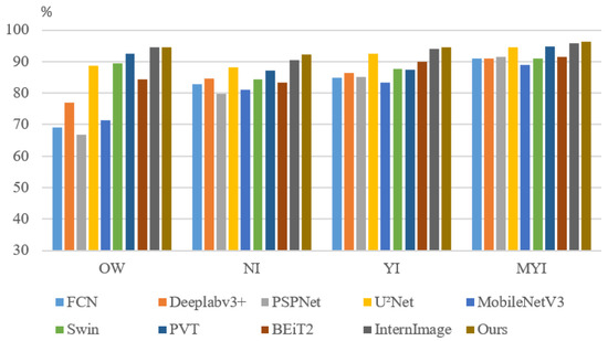
Figure 11.
CPA’s comparison of different backbones.
To further elucidate the differences between the proposed approach and classical semantic segmentation models, Figure 12 presents qualitative visual comparisons. The proposed GLDCN produces more accurate segmentations than competing methods. Although InternImage and GLDCN yield boundaries that are closer to the manually annotated ground truth, for the MYI–YI discrimination shown in Figure 12c, GLDCN achieves a higher level of discriminability.
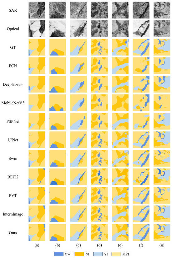
Figure 12.
Comparison of segmentation results from different backbones. (a–g) are seven ice chart samples randomly selected.
In addition, we conduct a complexity comparison among models with superior performance across various metrics, including PA, mIoU, and Kappa coefficient, as shown in Table 2. The BEiT2 model, based on the ViT architecture, exhibits a notably high parameter count of 323.66 M, significantly exceeding that of other models. In contrast, the proposed model achieves the best results across all three evaluation metrics while maintaining a parameter count of approximately 102.76 M and FLOPs of around 17.51 G, which are considerably lower than those of large-parameter models such as BEiT2. Compared with lightweight models like U2Net, Swin, and InternImage, our model demonstrates superior overall performance while retaining comparable parameter and computational complexity. This indicates that our model effectively balances accuracy and complexity, demonstrating high potential for practical applications.
Table 2.
Comparison of model computational complexity.
4.3. Comparison Experiments on the Fusion Module
To evaluate the effectiveness of the proposed ACAM fusion module in integrating SAR and optical image information, comparative experiments are conducted based on the GLDCN backbone using several mainstream fusion strategies, including SFF [35], DAB [36], and a conventional convolution-based fusion module. As shown in Table 3, ACAM achieves the highest performance, with PA, mIoU, and Kappa coefficient values of 95.99%, 91.3%, and 93.99%, respectively. These results demonstrate the superior overall classification capability of the proposed approach. Figure 13 shows each module over the baseline in PA, mIoU, and the Kappa coefficient, providing a more intuitive illustration of this point.
Table 3.
Performance comparison of fusion models.
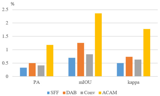
Figure 13.
The improvements in each module over the baseline in PA, mIoU, and the Kappa coefficient.
In particular, ACAM surpasses the second-best module by 1.10% in mIoU and 1.04% in the Kappa coefficient, confirming its effectiveness in capturing inter-class distinctions and mitigating class imbalance issues. Figure 14 further illustrates this advantage from a category-wise perspective: ACAM consistently maintains the highest classification accuracy in all four categories of sea ice, with the most pronounced improvement observed for NI. This improvement can be attributed to ACAM’s enhanced ability to fuse fine-grained local details with broader contextual information, thereby enabling more accurate perception and discrimination of morphologically diverse NI types.
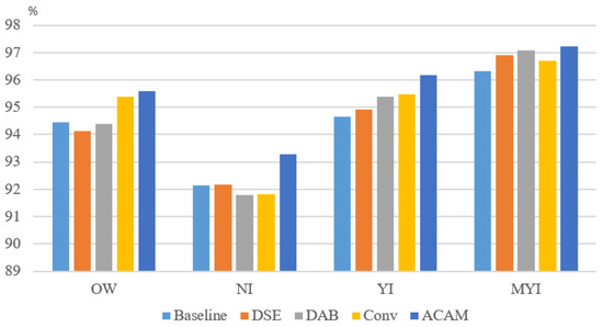
Figure 14.
CPA’s comparison of different fusion modules.
4.4. Ablation Experiments on Data
To validate the effectiveness of multi-polarization SAR feature and the necessity of multi-source data fusion, data-level ablation experiments are conducted in this study. The dataset is divided into five groups, with the proposed GLDCN model employed as the backbone. The fifth data uses the ACAM fusion module. The data groups are defined as follows:
- Group 1: Single-polarization SAR data (HH)
- Group 2: Full-polarization SAR data (HH/HV/VV)
- Group 3: All SAR information (HH/HV/VV + typical polarization features)
- Group 4: Optical data
- Group 5: Fusion of all SAR information and optical data
The experimental results are presented in Table 4. The overall and class-wise performance of the model improves significantly as the input data increases. When only single-polarization HH data are used, the model achieves the lowest overall performance, indicating that a single scattering feature is insufficient to effectively distinguish structurally complex sea ice types. After introducing full-polarization information (HH/HV/VV), the model exhibits a substantial performance improvement, with PA, mIoU, and Kappa coefficient increasing by 6.84%, 10.51%, and 10.31%, respectively. This demonstrates that different polarization modes can better capture sea ice texture and scattering characteristics. With the inclusion of PRCPs and PDPs, the classification accuracy for the OW category increases markedly, suggesting that decomposed polarimetric features strengthen the differentiation between seawater and various sea ice types. Comparing Group 3 and Group 4, we observe that SAR and optical data each have their own advantages across different categories. For the NI class, the accuracy of optical data exceeds that of SAR data by 3.62%, while for the YI and MYI classes, SAR data performs better. From a physical mechanism perspective, we explain the respective advantages of optical and SAR images in sea ice classification. For SAR images, NI surfaces have relatively low roughness, resulting in overall low backscatter intensity, which can easily be confused with the OW category. In contrast, optical images have strong spectral recognition abilities for new ice, often appearing dark gray or dark blue in the images, creating a noticeable color difference from the surrounding black water. For the YI and MYI categories, the extracted polarization features provide additional information, making SAR data slightly superior to optical data. This indicates strong complementarity between the two data sources.
Table 4.
Performance comparison of different data.
Finally, the deep fusion of SAR and optical data achieves the most comprehensive and balanced performance, with PA, mIoU, and Kappa coefficient values of 95.99%, 91.3%, and 93.99%, respectively. More importantly, the CPA for four sea ice categories reaches its highest level after fusion, verifying the critical importance of data complementarity.
Figure 15 and Figure 16 show the comparison of CPA and segmentation visualizations under different data. As illustrated, the classification performance with multi-polarization data is significantly superior to that with single-polarization data. As shown in Figure 16c, in distinguishing OW and NI, the results incorporating polarimetric features outperform those without them, indicating that the extracted polarimetric features effectively capture subtle differences between sea ice and adjacent water regions. A comparison between Figure 16a,f further reveals that optical data perform better in identifying NI, whereas SAR data show a clear advantage in recognizing YI. This observation is consistent with the quantitative results presented in Table 4. Notably, when SAR and optical data are fused, the model achieves further improvements in the classification performance for these ice types. The fusion also enhances the delineation of complex boundary regions, leading to accurate and robust sea ice semantic segmentation.
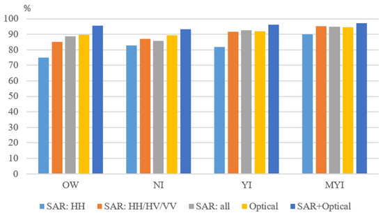
Figure 15.
CPA’s comparison of different data.
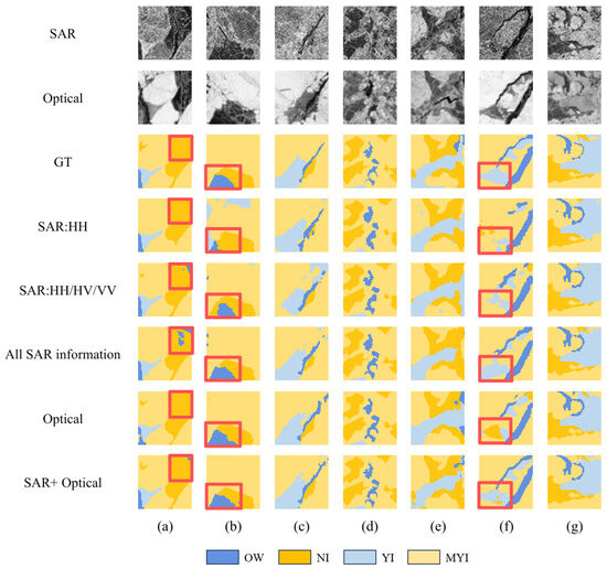
Figure 16.
Comparison of segmentation results on different data. (a–g) are seven ice chart samples randomly selected.
5. Conclusions
Focusing on the task of sea ice classification under complex conditions, this paper proposes a deep learning algorithm for sea ice classification by integrating GaoFen-3 fully polarimetric SAR and Landsat optical data. During the data processing stage, we extract 13 polarimetric features from GaoFen-3 fully polarimetric SAR data to characterize the textural information of sea ice, and build a high-quality sea ice dataset by matching with Landsat optical imagery. For the backbone network, this paper introduces the GLDCN that integrates global and local features and achieves long-range semantic association in a lightweight manner to improve accuracy at boundaries. GLDCN outperforms mainstream semantic segmentation models on multiple evaluation metrics, demonstrating exceptional feature extraction and contextual modeling capabilities. In the heterogeneous data fusion component, this paper proposes an ACAM fusion module to dynamically adopt the contributions of optical and SAR features. By effectively utilizing their complementary characteristics, the module achieves robust cross-modal integration, thereby enhancing the accuracy of sea ice classification. Based on the proposed ACA-GLDCN framework, we conduct data ablation studies. Experimental results indicate that the incorporation of polarimetric features (PRCPs and PDPs) enhances the model’s capability to distinguish between open water and different sea ice types, validating the effectiveness of polarimetric information. Furthermore, the deep fusion of optical and SAR data achieves optimal performance for all sea ice categories, further confirming the necessity of multi-source data fusion. This research provides a new technical method for the intelligent interpretation of multi-source remote sensing data in complex sea ice scenarios, with positive implications for navigation planning and climate studies. Future work will focus on exploring the model’s generalization capability across regions and seasons, and attempt to incorporate temporal information to enhance the modeling of sea ice dynamic evolution processes.
Author Contributions
Conceptualization, F.J. and W.Z.; methodology, F.J. and X.Y.; software, F.J.; validation, X.Y., J.Z. and Q.C.; formal analysis, F.J., W.Z. and J.Z. investigation, F.J., G.L. and S.H.; resources, J.Z. and Q.C.; data curation, F.J. and X.Y.; writing—original draft preparation, F.J.; writing—review and editing, W.Z. and X.Y.; visualization, F.J.; supervision, G.L.; project administration, W.Z. and J.Z.; funding acquisition, W.Z. All authors have read and agreed to the published version of the manuscript.
Funding
This research was supported by the “Thirteenth Five-Year Plan” Record Subsystem Program.
Data Availability Statement
The GaoFen-3 and Landsat satellite data used in this study are available from the respective data providers. The processed multi-source sea ice dataset built by the authors is available upon reasonable request.
Acknowledgments
The authors extend their sincere gratitude for the data support from the GaoFen-3 and Landsat satellite programs, as well as the ice chart products provided by the U.S. National Ice Center, which are essential for the experiments of the study.
Conflicts of Interest
The authors declare no conflicts of interest.
References
- Cai, Q.; Wang, J.; Beletsky, D.; Overland, J.; Ikeda, M.; Wan, L. Accelerated decline of summer Arctic sea ice during 1850–2017 and the amplified Arctic warming during the recent decades. Environ. Res. Lett. 2021, 16, 034015. [Google Scholar] [CrossRef]
- Liu, Z.; Risi, C.; Codron, F.; He, X.; Poulsen, C.; Wei, Z.; Chen, D.; Li, S.; Bowen, G. Acceleration of western Arctic sea ice loss linked to the Pacific North American pattern. Nat. Commun. 2021, 12, 1519. [Google Scholar] [CrossRef]
- Zhang, F.; Lei, R.; Zhai, M.; Pang, X.; Li, N. The impacts of anomalies in atmospheric circulations on Arctic sea ice outflow and sea ice conditions in the Barents and Greenland seas: Case study in 2020. Cryosphere 2023, 17, 4609–4628. [Google Scholar] [CrossRef]
- He, L.; He, X.; Hui, F.; Ye, Y.; Zhang, T.; Cheng, X. Investigation of Polarimetric Decomposition for Arctic Summer Sea Ice Classification Using Gaofen-3 Fully Polarimetric SAR Data. IEEE J. Sel. Top. Appl. Earth Obs. Remote Sens. 2022, 15, 3904–3915. [Google Scholar] [CrossRef]
- Zhang, T.; Yang, Y.; Shokr, M.; Mi, C.; Li, X.; Cheng, X.; Hui, F. Deep Learning Based Sea Ice Classification with Gaofen-3 Fully Polarimetric SAR Data. Remote Sens. 2021, 13, 1452. [Google Scholar] [CrossRef]
- Li, W.; Liu, L.; Zhang, J. Fusion of SAR and optical image for sea ice Extraction. J. Ocean. Univ. China 2021, 20, 1440–1450. [Google Scholar] [CrossRef]
- Zhao, L.; Xie, T.; Perrie, W.; Yang, J. Deep-Learning-Based Sea Ice Classification with Sentinel-1 and AMSR-2 Data. IEEE J. Sel. Top. Appl. Earth Obs. Remote Sens. 2023, 16, 5514–5525. [Google Scholar] [CrossRef]
- Wiehle, S.; Murashkin, D.; Frost, A.; König, C.; König, T. Sea Ice Classification Using Combined Sentinel-1 and Sentinel-3 Data. In Proceedings of the IGARSS 2024—2024 IEEE International Geoscience and Remote Sensing Symposium, Athens, Greece, 7–12 July 2024; pp. 102–106. [Google Scholar] [CrossRef]
- Wu, G.; Yang, X.; Liang, H.; Luo, J.; Lang, W. PID Controllers Guided Multitask Sea Ice Inversion Approach of SAR and Amsr-2 Images Based on Convolutional Neural Network. In Proceedings of the IGARSS 2024—2024 IEEE International Geoscience and Remote Sensing Symposium, Athens, Greece, 7–12 July 2024; pp. 61–64. [Google Scholar] [CrossRef]
- Boulze, H.; Korosov, A.; Brajard, J. Classification of Sea Ice Types in Sentinel-1 SAR Data Using Convolutional Neural Networks. Remote Sens. 2020, 12, 2165. [Google Scholar] [CrossRef]
- Xu, Y.; Scott, K.A. Sea ice and open water classification of sar imagery using cnn-based transfer learning. In Proceedings of the 2017 IEEE International Geoscience and Remote Sensing Symposium (IGARSS), Fort Worth, TX, USA, 23–28 July 2017; pp. 3262–3265. [Google Scholar] [CrossRef]
- Zhang, J.; Zhang, W.; Hu, Y.; Chu, Q.; Liu, L. An Improved Sea Ice Classification Algorithm with Gaofen-3 Dual-Polarization SAR Data Based on Deep Convolutional Neural Networks. Remote Sens. 2022, 14, 906. [Google Scholar] [CrossRef]
- Zhao, J.; Chen, L.; Li, J.; Zhao, Y. Semantic Segmentation of Sea Ice Based on U-net Network Modification. In Proceedings of the 2022 IEEE International Conference on Robotics and Biomimetics (ROBIO), Jinghong, China, 5–9 December 2022; pp. 1151–1156. [Google Scholar] [CrossRef]
- Ren, Y.; Xu, H.; Liu, B.; Li, X. Sea Ice and Open Water Classification of SAR Images Using a Deep Learning Model. In Proceedings of the IGARSS 2020—2020 IEEE International Geoscience and Remote Sensing Symposium, Waikoloa, HI, USA, 26 September–2 October 2020; pp. 3051–3054. [Google Scholar] [CrossRef]
- Ren, Y.; Li, X.; Yang, X.; Xu, H. Development of a Dual-Attention U-Net Model for Sea Ice and Open Water Classification on SAR Images. IEEE Geosci. Remote Sens. Lett. 2022, 19, 4010205. [Google Scholar] [CrossRef]
- Zhang, J.; Zhang, W.; Zhou, X.; Chu, Q.; Yin, X.; Li, G.; Dai, X.; Hu, S.; Jin, F. CNN and Transformer Fusion Network for Sea Ice Classification Using GaoFen-3 Polarimetric SAR Images. IEEE J. Sel. Top. Appl. Earth Obs. Remote Sens. 2024, 17, 18898–18914. [Google Scholar] [CrossRef]
- Cloude, S.; Pottier, E. A review of target decomposition theorems in radar polarimetry. IEEE Trans. Geosci. Remote Sens. 1996, 34, 498–518. [Google Scholar] [CrossRef]
- Freeman, A.; Durden, S. A three-component scattering model for polarimetric SAR data. IEEE Trans. Geosci. Remote Sens. 1998, 36, 963–973. [Google Scholar] [CrossRef]
- Shokr, M.; Dabboor, M. Polarimetric SAR Applications of Sea Ice: A Review. IEEE J. Sel. Top. Appl. Earth Obs. Remote Sens. 2023, 16, 6627–6641. [Google Scholar] [CrossRef]
- Yommy, A.S.; Liu, R.; Wu, S. SAR Image Despeckling Using Refined Lee Filter. In Proceedings of the 2015 7th International Conference on Intelligent Human-Machine Systems and Cybernetics, Hangzhou, China, 26–27 August 2015; Volume 2, pp. 260–265. [Google Scholar] [CrossRef]
- Lanczos, C. An iteration method for the solution of the eigenvalue problem of linear differential and integral operators. J. Res. Natl. Bur. Stand. B 1950, 45, 255–282. [Google Scholar] [CrossRef]
- Wang, W.; Dai, J.; Chen, Z.; Huang, Z.; Li, Z.; Zhu, X.; Hu, X.; Lu, T.; Lu, L.; Li, H.; et al. InternImage: Exploring Large-Scale Vision Foundation Models with Deformable Convolutions. In Proceedings of the 2023 IEEE/CVF Conference on Computer Vision and Pattern Recognition (CVPR), Vancouver, BC, Canada, 18–22 June 2022; pp. 14408–14419. [Google Scholar]
- Ba, J.; Kiros, J.R.; Hinton, G.E. Layer Normalization. arXiv 2016, arXiv:1607.06450. [Google Scholar] [CrossRef]
- Vaswani, A.; Shazeer, N.M.; Parmar, N.; Uszkoreit, J.; Jones, L.; Gomez, A.N.; Kaiser, L.; Polosukhin, I. Attention is All you Need. In Proceedings of the Neural Information Processing Systems, Long Beach, CA, USA, 4–9 December 2017. [Google Scholar]
- Dosovitskiy, A.; Beyer, L.; Kolesnikov, A.; Weissenborn, D.; Zhai, X.; Unterthiner, T.; Dehghani, M.; Minderer, M.; Heigold, G.; Gelly, S.; et al. An Image is Worth 16×16 Words: Transformers for Image Recognition at Scale. arXiv 2020, arXiv:2010.11929. [Google Scholar]
- Liu, Z.; Lin, Y.; Cao, Y.; Hu, H.; Wei, Y.; Zhang, Z.; Lin, S.; Guo, B. Swin Transformer: Hierarchical Vision Transformer using Shifted Windows. In Proceedings of the 2021 IEEE/CVF International Conference on Computer Vision (ICCV), Virtual, 11–17 October 2021; pp. 9992–10002. [Google Scholar]
- Xiao, T.; Liu, Y.; Zhou, B.; Jiang, Y.; Sun, J. Unified Perceptual Parsing for Scene Understanding. In Proceedings of the European Conference on Computer Vision, Munich, Germany, 8–14 September 2018. [Google Scholar]
- Shelhamer, E.; Long, J.; Darrell, T. Fully Convolutional Networks for Semantic Segmentation. IEEE Trans. Pattern Anal. Mach. Intell. 2017, 39, 640–651. [Google Scholar] [CrossRef]
- Yang, Z.; Peng, X.; Yin, Z.; Yang, Z. Deeplabv3 plus-net for Image Semantic Segmentation with Channel Compression. In Proceedings of the 2020 IEEE 20th International Conference on Communication Technology (ICCT), Nanning, China, 28–31 October 2020; pp. 1320–1324. [Google Scholar] [CrossRef]
- Zhao, H.; Shi, J.; Qi, X.; Wang, X.; Jia, J. Pyramid Scene Parsing Network. In Proceedings of the 2017 IEEE Conference on Computer Vision and Pattern Recognition (CVPR), Honolulu, HI, USA, 21–26 July 2016; pp. 6230–6239. [Google Scholar]
- Qin, X.; Zhang, Z.; Huang, C.; Dehghan, M.; Zaiane, O.R.; Jägersand, M. U2-Net: Going Deeper with Nested U-Structure for Salient Object Detection. Pattern Recognit. 2020, 106, 107404. [Google Scholar] [CrossRef]
- Howard, A.G.; Sandler, M.; Chu, G.; Chen, L.C.; Chen, B.; Tan, M.; Wang, W.; Zhu, Y.; Pang, R.; Vasudevan, V.; et al. Searching for MobileNetV3. In Proceedings of the 2019 IEEE/CVF International Conference on Computer Vision (ICCV), Seoul, Republic of Korea, 27–28 October 2019; pp. 1314–1324. [Google Scholar]
- Wang, W.; Xie, E.; Li, X.; Fan, D.P.; Song, K.; Liang, D.; Lu, T.; Luo, P.; Shao, L. Pyramid Vision Transformer: A Versatile Backbone for Dense Prediction without Convolutions. arXiv 2021, arXiv:2102.12122. [Google Scholar] [CrossRef]
- Peng, Z.; Dong, L.; Bao, H.; Ye, Q.; Wei, F. BEiT v2: Masked Image Modeling with Vector-Quantized Visual Tokenizers. arXiv 2022, arXiv:2208.06366. [Google Scholar]
- Ma, X.; Zhang, X.; Pun, M.O.; Liu, M. A Multilevel Multimodal Fusion Transformer for Remote Sensing Semantic Segmentation. IEEE Trans. Geosci. Remote Sens. 2024, 62, 5403215. [Google Scholar] [CrossRef]
- Liu, S.; Li, F.; Zhang, H.; Yang, X.; Qi, X.; Su, H.; Zhu, J.; Zhang, L. DAB-DETR: Dynamic Anchor Boxes are Better Queries for DETR. arXiv 2022, arXiv:2201.12329. [Google Scholar] [CrossRef]


Disclaimer/Publisher’s Note: The statements, opinions and data contained in all publications are solely those of the individual author(s) and contributor(s) and not of MDPI and/or the editor(s). MDPI and/or the editor(s) disclaim responsibility for any injury to people or property resulting from any ideas, methods, instructions or products referred to in the content. |
© 2025 by the authors. Licensee MDPI, Basel, Switzerland. This article is an open access article distributed under the terms and conditions of the Creative Commons Attribution (CC BY) license.