Geospatial and Deep Learning Approaches for Modeling Floodwater Depth in Urbanized Areas

Highlights

What are the main findings?

• Lightweight ResNet-UNet accurately estimates flood depth under hydrostatic equilibrium conditions using remote sensing data.
• Incorporating DEM-derived terrain features improves mapping accuracy and spatial coherence.

What are the implications of the main findings?

• Feasible near-real time urban flood-depth water mapping to support rapid response.
• Effective in data-scarce regions, reducing reliance on in-situ measurements.

Abstract

Floodwater depth estimation is essential for disaster response and infrastructure planning yet remains challenging in urban areas with limited gage and hydrological data. This study presents a deep learning-based framework grounded in the hydrostatic equilibrium principle to estimate flood depth using a remote sensing approach. A series of ResNet architectures were trained and evaluated under two different scenarios: (a) a baseline model input using LiDAR-derived DTM and flood extent, and (b) an enhanced model incorporating additional terrain features such as slope, curvature, and Topographic Wetness Index (TWI). The results demonstrate that ResNet18 outperformed deeper models, achieving an RMSE of 0.71 ft, Huber Loss of 0.28 ft, MAE of 0.23 ft, SSIM of approximately 99% and R-Squared of approximately 94% under the enhanced scenario. Inclusion of terrain predictors led to significant improvements in prediction accuracy and spatial coherence. They improved Huber Loss by 28%, RMSE by 13%, and MAE by 21%. However, when applied to an unseen peri-urban catchment, model performance declined (RMSE = 1.95 ft), mainly due to limited and temporally misaligned ground truth data, and differences in spatial characteristics. Despite these limitations, ResNet18 generalizes well, mapping flood depth in unseen catchments, and demonstrates the potential for rapid assessments in data-scarce regions.

1. Introduction

Globally, the frequency, severity, and duration of flooding events are increasing due to the compounding effects of climate change, land use dynamics, and rapid urbanization [1]. Empirical evidence indicates that anthropogenic warming and land cover changes have significantly altered hydrological cycles, intensifying the magnitude and occurrence of extreme flood events. In urban environments, the situation is further exacerbated by inadequate drainage infrastructure, population growth, and expanding built-up areas, resulting in heightened exposure and vulnerability to flood hazards [1].

Global projections estimate that by 2100, 52% of the population and 46% of built assets will be at risk of severe flooding [2], with approximately 68% of new flood events expected to be driven by tidal and storm-related factors [3]. An estimated 1.8 billion people, about 23% of the world’s population, are directly exposed to floodwater depths exceeding 0.49 feet (0.15 m), placing vulnerable communities at significant risk [4]. In the United States, for instance, flooding from severe storms has consistently resulted in major economic impacts, particularly in urban and coastal areas. Hurricanes such as Harvey (2017) and Ian (2022) together caused damages exceeding USD 100 billion. More recently, Hurricane Helene (2024) alone caused approximately USD 78.7 billion in property damages [5].

While flood extent mapping has been widely studied, the estimation of floodwater depth, especially in urban areas, remains limited, despite its critical importance for impact assessment, risk analysis, and emergency response [6,7]. Floodwater depth has gained increasing attention in hydrological research, especially in urban areas where the consequences for infrastructure, the economy, and human life are often severe [8]. Impervious surfaces in cities limit rainfall infiltration, accelerating surface runoff during storms. This often intensifies urban flash floods, making them more destructive to building infrastructure and people, and posing challenges for sustainable and resilient development [9].

Traditionally, hydrodynamic models such as LISFLOOD, MIKE FLOOD, and others have been applied for simulating floodwater depth using various hydrological and hydraulic parameters. However, these models are computationally intensive and heavily constrained by the availability of high-quality data for calibration and validation, particularly in urban environments. These limitations stem from the sparse spatial distribution of monitoring equipment and the high cost associated with installing and maintaining ground-based gauging stations. Furthermore, urban environments are typically characterized by complex and fragmented waterlogging patterns caused by low-lying infrastructure such as subway entrances, underpasses, and tunnels, which are challenging to monitor using conventional sensor-based systems [8]. With recent extreme flood events exceeding the spatial and temporal extent of historical records, there is a critical need for spatially continuous and timely flood monitoring capabilities, which can be effectively addressed through remote sensing and deep learning techniques, which is the scope of this research.

Recent studies have increasingly adopted data-driven approaches, leveraging both traditional and non-traditional remote sensing and deep learning techniques to estimate of maximum floodwater depth in urban areas [1,3]. A growing body of research has utilized crowdsourced flood imagery (e.g., social media, web platforms), and deep convolutional neural networks to infer urban flood depth. Ref. [10] applied Mask R-CNN with traffic sign poles as scale references, yielding a mean absolute error (MAE) of 12.63 in. (1.05 ft) in floodwater depth estimation. Ref. [11] used a ResNet50 model with improved attention mechanisms for object-based floodwater depth estimation, outperforming other models such as GoogleNet and MobileNet-V2 in urban settings. Refs. [8,12] applied YOLOv8 and YOLOv4, respectively, to identify partially submerged objects such as vehicles and pedestrians to infer water depth, where a higher accuracy was achieved when vehicles were used due to their standardized dimensions. Ref. [13] introduced a Coordinate Attention-ResNet (CA-ResNet) model combined with social media imagery and IoT for similar purposes. Despite the advancements, these approaches are limited by their sensitivity to the reference object type, which may not be consistent across different geographies or flood events, dependency on image quality and availability, and limited spatial scalability [8].

In contrast other studies have explored terrain-informed learning using traditional remote sensing data. Ref. [14] trained a U-Net model on hyetographs and topographic variables to predict 2D floodwater depth maps, concluding that a model with approximately 28 million parameters performed better for depth prediction. Ref. [15] combined UAV imagery and digital terrain models (DTMs) with an FCN-8 architecture, achieving a root mean squared error (RMSE) of 0.26 m (0.85 ft) in floodwater depth prediction. Ref. [16] employed conditional Generative Adversarial Networks (cGAN), incorporating topography, land use, and rainfall data, reporting that their deep learning approach was approximately 250 times faster than HEC-RAS hydrodynamic models. Collectively, these studies highlight the value of integrating multi-source remote sensing and hydrologically relevant terrain data in deep learning frameworks.

While these studies represent important progress, a comprehensive framework that fuses high-resolution remote sensing data with deep learning architectures, informed by hydrological and topographical principles, remains underexplored. This study aims to fill that gap by developing and evaluating deep learning-based models for urban floodwater depth estimation that explicitly leverages hydrostatic principles and physically relevant variables derived from remote sensing sources. Our contribution is a practical regression framework that integrates flood-inundated extent with DTM and hydrologically relevant topographic features (e.g., slope, curvature, TWI) to produce interpretable and spatially coherent depth estimates in urban settings.

2. Materials and Methods

2.1. Hydrostatic Equilibrium Principle

This study is grounded in the principle of hydrostatic equilibrium, which describes the behavior of water at rest and its relationship with the underlying terrain. In the absence of significant momentum (i.e., during standing or slowly receding floodwaters), water conforms to the underlying topography, and its depth can be estimated using terrain elevation data. Thus, water at rest distributes itself according to the terrain and forms a relatively smooth surface and the floodwater depth at any location can be estimated as the vertical difference between the water surface elevation and the ground elevation at that point:

H(x, y) = W(x, y) − D(x, y),

where, H(x, y) is the floodwater depth at location (x, y), W(x, y) is the water surface elevation at location (x, y), and D(x, y) is the ground elevation at location (x, y).

By leveraging this relationship between a flood-inundated area and the underlying terrain, the study integrates geospatial data and remote sensing imagery with deep learning models to estimate post-floodwater depth. The use of this physical principle ensures that the predictions are both interpretable and constrained by real-world hydrological behavior.

Applicability to Urban Flood Conditions

While the hydrostatic equilibrium principle is strictly valid when water is stationary or receding slowly, urban flood environments often involve transient, momentum-driven flows, particularly during peak inundation [9]. In such conditions, local water surfaces may deviate from hydrostatic behavior due to dynamic effects such as rapid runoff, and stormwater infrastructure. However, the remote sensing imagery used in this study represents post-event conditions, when overland flow velocities have typically decreased and the flood water surface approaches quasi-static behavior. Consequently, applying the hydrostatic principle provides a reasonable approximation for estimating residual flood depths, though errors may arise in locations where flow remained energetic or where hydraulic controls (e.g., culverts, storm drains) induced non-hydrostatic water surfaces. These deviations generally manifest as local over- or under-estimations of depth. Therefore, our use of the hydrostatic assumption should be considered an approximate but physically interpretable constraint that stabilizes model predictions while acknowledging expected uncertainties introduced by complex urban hydraulics.

2.2. Research Data

Research data were sampled from 12 flood-affected urban and peri-urban areas in Southeastern United States, specifically within North Carolina and South Carolina (Figure 1). Sample sites were selected based on the severity of flood impact during two major hurricane events: Hurricane Matthew in 2016 and Hurricane Florence in 2018. These areas collectively span approximately 25,059 acres of developed land, representing diverse flood conditions across varying topographic and hydrologic settings to support robust model training and evaluation. The selection was also guided by the availability of high-resolution post-event remote sensing data, and ground-truth flood depth information. Nine of the sites were affected by Hurricane Matthew, while three were impacted by Hurricane Florence (Table 1).

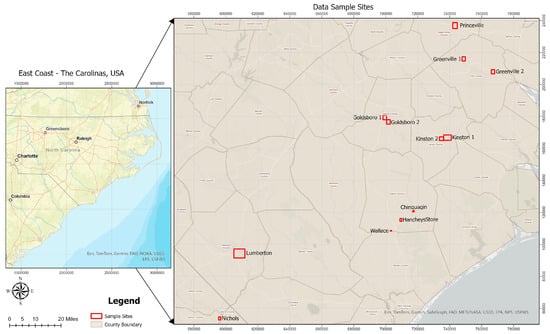
Figure 1. Overview of the East Coast with the spatial locations of the research data sample sites highlighted.

Table 1. Data sampling sites and their characteristics.

Site	Area (Acres)	Elevation (ft)	Hurricane Type
Lumberton	9496.55	148	Matthew
Kinston 1	3886.7	63	Matthew
Princeville	2597.82	53	Matthew
Goldsboro 2	1536.73	78	Matthew
Goldsboro 1	1510.81	94	Matthew
Kinston 2	1465.11	45	Matthew
Greenville 1	1377.24	36	Matthew
Greenville 2	1347.99	32	Matthew
Nichols	617.57	18	Matthew
Hancheys Store	534.85	42	Florence
Chinquaqin	217.41	43	Florence
Wallace	61.1	38	Florence

Post-flood aerial imagery, used to capture surface conditions shortly after the hurricanes, was obtained from the NOAA Storms Archive. For the study areas, imagery corresponding to Hurricane Matthew was acquired between 10 and 15 October 2016, and for Hurricane Florence, on 18 September 2018. They have a spatial resolution of approximately 0.25 m and cover only the affected settlement areas included in this study. Digital Terrain Models, derived from LiDAR point clouds, were sourced from the North Carolina Emergency Management Spatial Data Portal and the USGS 3D Elevation Program (3DEP), with a spatial resolution of approximately 1 m. Finally, High water Mark (HWM) data, collected by the Federal Emergency Management Agency (FEMA) in partnership with USGS after storm events, were used to provide reference floodwater depth measurements for evaluation. These datasets provided essential inputs for estimating floodwater depth with high spatial precision.

2.3. Data Processing

A workflow was developed to preprocess and integrate the multiple geospatial datasets to train and evaluate deep learning models for floodwater depth prediction across selected urban and peri-urban sites. The data processing framework combined post-event aerial imagery, DTMs, pre-trained deep learning frameworks and geostatistical techniques to generate input and reference variables for model training and evaluation (Figure 2).

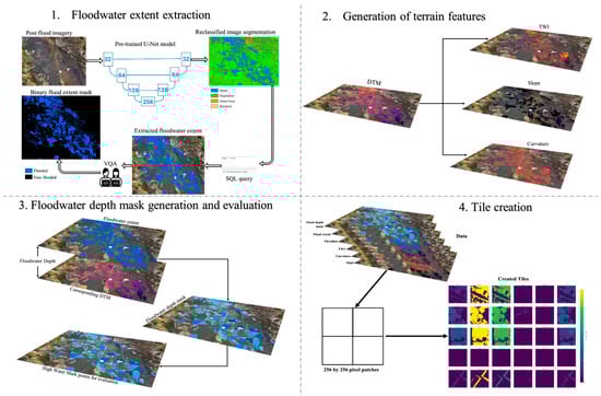
Figure 2. Data processing workflow.

In the first stage, we delineated flood-inundated areas from the post-flood aerial imagery. We employed Esri’s pre-trained U-Net–based High-Resolution Land-Cover Classification model, which is available in two configurations, one that predicts seven classes and another that predicts nine classes. We selected the nine-class configuration because it provides more detailed and elaborative land-cover categories, including ‘open water’, which supports more accurate flood delineation in heterogeneous urban environments. The model assigns each pixel to one of the nine predefined classes and does not include a background or “other” category [17].

The extracted flood extent was validated using a qualitative review supported by independent cross-checks against the original aerial imagery. Although the Esri High-Resolution Land-Cover model provides class-level accuracy metrics (Section 3), its pixel-wise “open water” predictions can still introduce omission (missed flooded areas) and commission (misclassified non-flooded areas) errors, particularly in shadowed regions, vegetated areas, and narrow street canyons. To address this, we performed systematic manual corrections following a standardized visual-assessment protocol, ensuring consistency across sites [18,19]. Therefore, the study acknowledge that the final flood-extent masks, while visually validated and manually corrected, retain inherent uncertainty that may influence the subsequent depth-estimation results (Figure 2).

In parallel, terrain characteristics, which induce hydrologic processes influencing floodwater distribution, were derived from the DTM datasets. The high resolution DTM, derived from the ground-based points of LiDAR 3D point cloud, provides detailed surface elevation information essential for terrain analysis. Terrain features such as elevation, slope, curvature, and topographic wetness index (TWI) were derived for each site to represent terrain-driven influences on flood behavior (Table 2). Then, the ground truth floodwater depth mask for each site was generated by integrating the segmented flood extent boundaries with the underlying DTM, in accordance with the hydrostatic equilibrium principle (Section 2.1). In sites where available, FEMA HWM data were used to validate and calibrate these estimated depths. Due to the lack of high-quality reference depth mask in these areas, these HWM ground-based observations served as reference points to assess the accuracy of the floodwater depth masks (Section 3). Manual validation and spatial querying techniques were also employed to refine the results and enhance the spatial accuracy of training masks used in the deep learning pipeline (Figure 3).

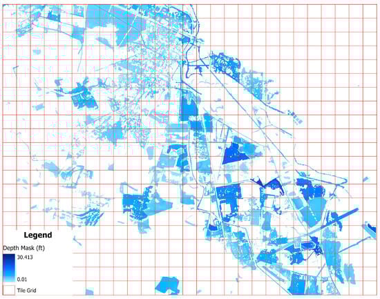
Figure 3. Sample ground-truth depth mask with overlayed 256 by 256 grids for Lumberton.

To prepare the data for model training and evaluation, all generated data layers, including the flood extent masks, DTM-derived features (elevation, slope, curvature, etc.), and the ground truth flood depth mask), were spatially aligned using a common coordinate system, and resampled to a uniform 1 m resolution. All feature layers were normalized to the $[0, 1]$ range using global min–max scaling, where the minimum and maximum values were computed across the entire dataset rather than on a per-tile basis [19]. This ensures consistent scaling of elevation, terrain derivatives, and flood-related features across all study areas and prevents tile-wise normalization from introducing artificial differences between patches (Table 2). These layers were then subdivided into standardized tiles to enable efficient model ingestion using the ezprocess library [20]. Specifically, each raster was split into 256 by 256 pixel patches to ensure consistent input dimensions for the neural network and to optimize batch processing during training. The tiles were generated with a 128-pixel overlap between adjacent patches, which helped preserve spatial continuity across tile boundaries and increased the training sample size by capturing edge effects and transitional zones. This overlap also supported better learning of localized terrain transitions that influence floodwater accumulation. In total, 5925 tiles were generated from the processed datasets across all sample locations (Figure 4).

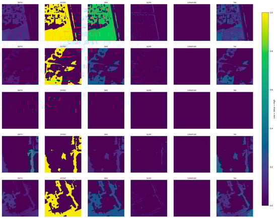
Figure 4. Sample 256 by 256 generated tiles for various features.

We implemented Quality Control (QC) and Quality Assurance (QA) for terrain and imagery (e.g., spike removal in DTM, mask topology, visual audits, HWM cross-validation and temporal misalignment, and checks for georeferencing). Because HWMs were collected after the imagery and water levels likely receded in the interim, errors computed at the pixel level against HWMs may overstate the true image-time error; we therefore interpret them as upper bounds. We further masked obviously inconsistent pixels (e.g., vegetation-induced DTM artifacts) before tiling, to reduce label noise.

Table 2. Variables and their role in floodwater depth estimation.

Raster Variable	Scale	Role in Floodwater Depth Estimation
Flood Extent	Binary [0, 1]	Indicates areas within the delineated flood boundary (1) and areas outside it (0), Used to spatially constrain flood depth prediction to inundated zones. Referenced in [21,22].
DTM (Elevation)	Scaled to [0, 1]	Captures ground surface elevation, excluding above-ground structures. The datasets were scaled using MinMax normalization. Areas outside flood extent are also set to 0. Referenced in [14,23].
Topographic Wetness Index (TWI)	Scaled to [0, 1]	Measures the potential of a location to accumulate runoff based on upslope area and slope. It was estimated using the formular TWI = ln(a/tan β), where, a is the area drained at a point in sq.ft and tan β is the slope angle in radians. The datasets were scaled using MinMax normalization. Areas outside flood extent are also set to 0. Referenced in [24].
Curvature	Scaled to [0, 1]	Describes surface convexity or concavity, which influences local pooling. The datasets were scaled using MinMax normalization. Areas outside flood extent are also set to 0. Referenced in [25,26].
Slope	Scaled to [0, 1]	Quantifies terrain steepness. Flatter areas are more prone to water accumulation. The datasets were scaled using MinMax normalization. Areas outside flood extent are also set to 0. Referenced in [16,27].
Flood Depth Mask	Scaled to [0, 1]	Represents the reference floodwater depth within inundated areas. Used as the ground truth in supervised model training. The datasets were scaled using MinMax normalization. Areas outside flood extent are also set to 0. Referenced in [19].

Table 2. Variables and their role in floodwater depth estimation.

Raster Variable	Scale	Role in Floodwater Depth Estimation
Flood Extent	Binary [0, 1]	Indicates areas within the delineated flood boundary (1) and areas outside it (0), Used to spatially constrain flood depth prediction to inundated zones. Referenced in [21,22].
DTM (Elevation)	Scaled to [0, 1]	Captures ground surface elevation, excluding above-ground structures. The datasets were scaled using MinMax normalization. Areas outside flood extent are also set to 0. Referenced in [14,23].
Topographic Wetness Index (TWI)	Scaled to [0, 1]	Measures the potential of a location to accumulate runoff based on upslope area and slope. It was estimated using the formular TWI = ln(a/tan β), where, a is the area drained at a point in sq.ft and tan β is the slope angle in radians. The datasets were scaled using MinMax normalization. Areas outside flood extent are also set to 0. Referenced in [24].
Curvature	Scaled to [0, 1]	Describes surface convexity or concavity, which influences local pooling. The datasets were scaled using MinMax normalization. Areas outside flood extent are also set to 0. Referenced in [25,26].
Slope	Scaled to [0, 1]	Quantifies terrain steepness. Flatter areas are more prone to water accumulation. The datasets were scaled using MinMax normalization. Areas outside flood extent are also set to 0. Referenced in [16,27].
Flood Depth Mask	Scaled to [0, 1]	Represents the reference floodwater depth within inundated areas. Used as the ground truth in supervised model training. The datasets were scaled using MinMax normalization. Areas outside flood extent are also set to 0. Referenced in [19].

2.4. Deep Learning Models

To achieve the objective of this study, we compare CNN-based models and a transformer based model under various experimental setups. CNNs and transformer-based models differ in how they capture spatial information. CNNs use local filters, building global context gradually, which makes them efficient for tasks with strong local patterns. Transformers, like Swin UNet, rely on self-attention to model long-range dependencies from the start, enabling richer contextual learning but often requiring more data or pretraining.

2.4.1. CNN-Based Models

Three residual neural networks (ResNet) architectures, ResNet-18, ResNet-34, and ResNet-50, were employed. These models contain approximately 11.7 million, 21.8 million and 25.6 million parameters, respectively. ResNet models are designed based on a residual learning framework that uses identity shortcut connections, which allow gradients to propagate more effectively during backpropagation and support the training of deeper networks [28]. Their capacity to learn both shallow and deep features simultaneously, makes them well suited for spatially complex tasks like floodwater depth predictions where both local and global spatial context are important.

Each model was adapted to perform regression task by modifying the fully connected classification layers to output continuous floodwater depth values. Also, the models were configured to accept multi-channel input tensors which comprises of spectral, topographic, and surface condition information, allowing the models to learn intricate relationships between observed inundation and physical terrain characteristics. These models were selected to examine how increasing network depth influences prediction accuracy across complex and heterogeneous urban flood environments.

2.4.2. Transformer-Based Model

The Swin UNet model [29] was employed as a transformer-based alternative to the CNN-based baselines (ResNet-18, ResNet-34, ResNet-50). Swin UNet builds on the Swin Transformer backbone [30] and applies shifted window self-attention, which helps the model to efficiently capture both local and global patterns in the data. This design improve scalability by combining hierarchical design with localized attention windows, making them well suited for high-resolution geospatial tasks such as flood depth estimation.

We utilized a pretrained Swin UNet encoder initialized with ImageNet weights. The original segmentation head was replaced with a regression module consisting of a single convolutional layer to produce a continuous-valued flood depth output. The model was trained end-to-end using standard regression objectives. The model leveraged a hierarchical encoder-decoder design based on the Swin Transformer framework, incorporating four levels of depth with progressively increasing attention heads (2, 4, 8, 8) and consistent patch-wise self-attention via shifted windows of size 8 × 8. Each encoder and decoder stage utilizes two Swin Transformer blocks, enabling local-global context aggregation with reduced computational overhead.

2.5. Performance Metrics

To assess the accuracy and reliability of the deep learning models in both training and evaluation phases, various quantitative metrics were employed, tailored to the regression nature of the floodwater depth prediction. These metrics were selected to capture both pixel-level numerical errors and structural agreement between predicted and reference flood depth maps. The indicators include regression-based error measures, such as Mean Absolute Error (MAE), Root Mean Squared Error (RMSE), and Huber Loss, which quantify the magnitude and distribution of prediction errors, as well as perceptual and statistical similarity metrics like the Structural Similarity Index (SSIM) and the coefficient of determination (R-Squared). Each metric provides a complementary perspective, enabling a comprehensive evaluation of both the precision and the structural fidelity of the model outputs (Table 3).

Table 3. Performance metrics and their characteristics.

Metric	Meaning	Formular	Range	Best Value
RMSE (Root Mean Squared Error)/L2 Loss [14]	Measures the average squared deviation of predicted depth maps. It is sensitive to outliers.	$\sqrt{(1/\mathrm{n})\ast \mathsf{\Sigma }({\mathrm{y}}_{\mathrm{i}}-{\hat{\mathrm{y}}}_{\mathrm{i}}{)}^2}$ where: ${\hat{\mathrm{y}}}_{\mathrm{i}}$: predicted depth value at location i. ${\mathrm{y}}_{\mathrm{i}}$: reference (ground truth) depth value at location i. n: $\mathrm{n}\mathrm{u}\mathrm{m}\mathrm{b}\mathrm{e}\mathrm{r} \mathrm{o}\mathrm{f} \mathrm{o}\mathrm{b}\mathrm{s}\mathrm{e}\mathrm{r}\mathrm{v}\mathrm{a}\mathrm{t}\mathrm{i}\mathrm{o}\mathrm{n}\mathrm{s}$.	0 to ∞	0
MAE (Mean Absolute Error)/L1 Loss [31]	Measures the average absolute deviation of predicted depth maps. It is less sensitive to outliers.	(1/n) ∗ Σ|yi − ${\hat{\mathrm{y}}}_{\mathrm{i}}$| where: ${\hat{\mathrm{y}}}_{\mathrm{i}}$: predicted depth value at location i. ${\mathrm{y}}_{\mathrm{i}}$: reference (ground truth) depth value at location i. n: $\mathrm{n}\mathrm{u}\mathrm{m}\mathrm{b}\mathrm{e}\mathrm{r} \mathrm{o}\mathrm{f} \mathrm{o}\mathrm{b}\mathrm{s}\mathrm{e}\mathrm{r}\mathrm{v}\mathrm{a}\mathrm{t}\mathrm{i}\mathrm{o}\mathrm{n}\mathrm{s}$.	0 to ∞	0
Huber Loss [32]	Combines the strengths of the MAE and RMSE for handling prediction errors. It is less sensitive to outliers but also penalizes minor errors.	$HL(y, \hat{\mathrm{y}})=\left\{\begin{array}{c}{\displaystyle \frac{1}{2}}{\left(y-\hat{\mathrm{y}}\right)}^2 if \left|y-\hat{\mathrm{y}}\right|\le \delta \\ \delta \left(\left|y-\hat{\mathrm{y}}\right|-{\displaystyle \frac{1}{2}}\delta \right) otherwise\end{array}\right.$ where: $\hat{\mathrm{y}}$: predicted depth value. $\mathrm{y}$: reference (ground truth) depth value. $\mathsf{\delta }$: threshold parameter.	0 to ∞	0
SSIM (Structural similarity index Measure) [32]	Evaluates the structural similarity between predicted and reference depth maps. It considers luminance, contrast, and structure which help preserve structural details in depth prediction maps.	$SSIM({\mathrm{y}}_{\mathrm{i}},\overline{\mathrm{y}})={\displaystyle \frac{(2{\mu }_y{\mu }_{\hat{\mathrm{y}}}+C_1)(2{\sigma }_{y\hat{\mathrm{y}}}+C_2)}{({\mu }_y^2+{\mu }_{\hat{\mathrm{y}}}^2+C_1)({\sigma }_y^2+{\sigma }_{\hat{\mathrm{y}}}^2+C_2)}}$ where: $\hat{\mathrm{y}}$: predicted floodwater depth map. $\mathrm{y}$: reference (ground truth) depth map. ${\mathsf{\mu }}_{\mathrm{y}}{,\mathsf{\mu }}_{\hat{\mathrm{y}}}$: means of predicted and reference maps. ${\mathsf{\sigma }}_{\mathrm{y}}^2,{\mathsf{\sigma }}_{\hat{\mathrm{y}}}^2$: variances. ${\mathsf{\sigma }}_{\mathrm{y}\hat{\mathrm{y}}}$: covariance between predicted and reference maps. ${\mathrm{C}}_1,{\mathrm{C}}_2$: small constants for numerical stability	0 to 1	1
Coefficient of Determination (R-Squared) [32]	Measures the variations in the observed depth maps explained by the model. Act as an indicator of overall model fit.	${\mathrm{R}}^2=1-{\displaystyle \frac{{\sum }_{i=1}^n{\left({\mathrm{y}}_{\mathrm{i}}-{\hat{\mathrm{y}}}_{\mathrm{i}}\right)}^2}{{\sum }_{i=1}^n{\left({\mathrm{y}}_{\mathrm{i}}-{\overline{\mathrm{y}}}_{\mathrm{i}}\right)}^2}}$ where; ${\hat{\mathrm{y}}}_{\mathrm{i}}$: predicted floodwater depth at location i. ${\mathrm{y}}_{\mathrm{i}}:\mathrm{observed} \mathrm{floodwater} \mathrm{depth} \mathrm{at} \mathrm{location}\mathrm{i}$. ${\overline{\mathrm{y}}}_{\mathrm{i}}:\mathrm{m}\mathrm{e}\mathrm{a}\mathrm{n} \mathrm{o}\mathrm{f} \mathrm{a}\mathrm{l}\mathrm{l} \mathrm{o}\mathrm{b}\mathrm{s}\mathrm{e}\mathrm{r}\mathrm{v}\mathrm{e}\mathrm{d} \mathrm{f}\mathrm{l}\mathrm{o}\mathrm{o}\mathrm{d}\mathrm{w}\mathrm{a}\mathrm{t}\mathrm{e}\mathrm{r} \mathrm{d}\mathrm{e}\mathrm{p}\mathrm{t}\mathrm{h} \mathrm{v}\mathrm{a}\mathrm{l}\mathrm{u}\mathrm{e}\mathrm{s}.$ $\mathrm{n}:\mathrm{n}\mathrm{u}\mathrm{m}\mathrm{b}\mathrm{e}\mathrm{r} \mathrm{o}\mathrm{f} \mathrm{o}\mathrm{b}\mathrm{s}\mathrm{e}\mathrm{r}\mathrm{v}\mathrm{a}\mathrm{t}\mathrm{i}\mathrm{o}\mathrm{n}\mathrm{s}$.	−∞ to 1	1

2.6. Model Implementation

All the models were implemented using a supervised regression framework to estimate floodwater depth from the spatial raster inputs (Figure 5). To evaluate the contribution of topographic complexity, model training was structured around two experimental scenarios: (1) a baseline model using only flood extent masks and Digital Terrain Models (DTMs), and (2) an extended model incorporating additional terrain-derived predictors such as slope, curvature, and the Topographic Wetness Index (TWI). This approach allowed for a controlled assessment of how additional terrain characteristics affect model performance and spatial generalization across complex flood-affected environments.

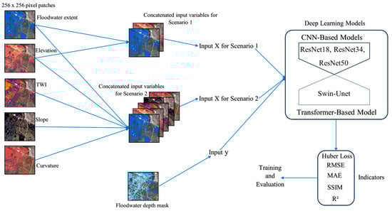
Figure 5. Model implementation workflow and training strategies.

The total 5925 generated tiles were split into training and evaluation subsets using a 60/40 train-test split. Specifically, 3555 tiles (60%) were used for model training, while the remaining 2370 tiles (40%) were evenly divided for validation (1185 tiles) and testing (1185 tiles). All models were trained for 200 epochs with a batch size of 8, selected after comparative test against alternate sizes (4, 16, 32). A learning rate of 1 × 10⁻⁴ was adopted based on preliminary trials with values such as 1 × 10⁻³, 1 × 10⁻⁵ and 1 × 10⁻³ with learning rate decay. The Huber Loss function was adopted for training, due to its robustness against outliers and combined sensitivity to small and large residuals, making it well suited for spatially complex flood depth predictions. Performance was assessed using the evaluation metrics (Table 3).

3. Results

We summarize key evaluation metrics for the datasets used in this study. Table 4 reports the per-class performance of the pretrained U-Net used to segment post-flood aerial imagery [17], while Table 5 presents site-level RMSE and MAE (ft) for our ground-truth depth mask evaluated against HWM observations. It is important to note that the number of samples are determined by the availability of HWM observations.

Table 4. Per class segmentation metrics of the pretrained U-Net model [20].

Class	Precision	Recall	F1 Score
Open Water	0.94	0.93	0.93
Wetlands	0.82	0.76	0.79
Tree Canopy	0.90	0.93	0.92
Shrubland	0.52	0.19	0.27
Low Vegetation	0.86	0.87	0.86
Barren	0.67	0.51	0.58
Structures	0.81	0.85	0.83
Impervious Surfaces	0.74	0.69	0.71
Impervious Roads	0.76	0.81	0.79

Table 5. Ground-truth Depth mask errors (RMSE, MAE in feet) at HWM validation sites.

Sample Site	RMSE (ft)	MAE (ft)	Number of Samples
Lumberton	2.48	1.65	27
Goldsboro 1	0.28	0.22	22
Goldsboro 2	0.86	0.85	22
Nichols	2.18	2.01	10
Hancheys Store	1.85	1.51	4
Chinquaqin	2.53	1.93	2
Wallace	2.35	2.33	2

Model training was executed on a high-performance server equipped with an AMD Ryzen Threadripper PRO 5955WX (16-core) CPU, 258 GB RAM, and an NVIDIA RTX A6000 GPU, leveraging CUDA 12.8. All implementations were optimized for GPU acceleration to ensure efficient convergence across model variants and input scenarios. The same hardware was used for catchment-scale deployment.

The models learned to infer floodwater depth by exploiting elevation differentials within the inundated zones, as constrained by the binary flood extent mask. This approach aligns with the hydrostatic equilibrium principle (Section 3.1). In this context, the DTM functions as the primary explanatory variable, and the flood extent mask delineates the spatial boundary within which the model estimates water depth. All the models across both training scenarios exhibited stable and consistent convergence behavior throughout the training epochs (Figure 6 and Figure 7). Using the selected hyperparameters (batch size = 8, learning rate = 0.0001, and the Huber loss function) the models achieved rapid early-stage convergence followed by gradual refinement, especially for the ResNet18 architecture (Figure 6).

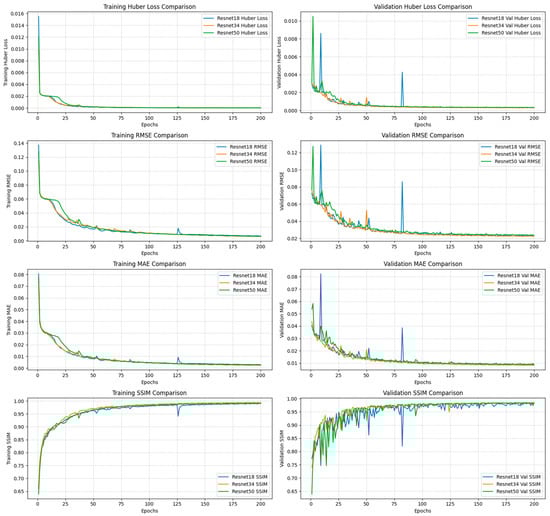
Figure 6. CNN-based models’ training and validation performance plots for scenario 1 baseline models.

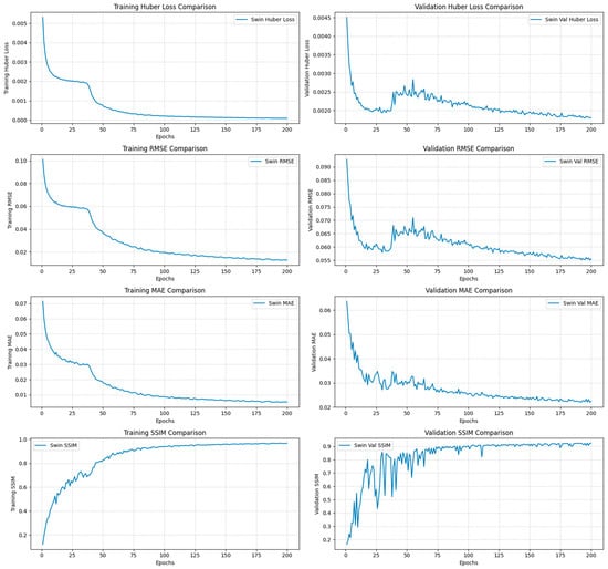
Figure 7. Swin-Unet transformer model training and validation performance plots for scenario 1 baseline models.

3.1. Scenario 1: Baseline Model Using Flood Extent and DTM

In the baseline scenario, floodwater depth was estimated using only flood extent mask and elevation as inputs. Despite the minimal input configuration, all three CNN-based ResNet and the Swin U-Net models achieved relatively strong predictive performance, demonstrating the foundational role of ground elevation in controlling floodwater behavior under hydrostatic conditions.

Among the tested architectures, ResNet34 consistently outperformed the other models, achieving the lowest RMSE (0.74 ft) and MAE (0.27 ft), alongside and highest SSIM (98.5%) and R-Squared (93%) scores (Table 6). By comparison, ResNet18 and ResNet50 recorded slightly higher prediction errors, with RMSE values of 0.82 ft and 0.83 ft, and MAE values of 0.29 ft and 0.30 ft, respectively. Their corresponding SSIM (both 98.3%) and R-Squared (both 91%) scores showed lower structural and statistical agreement between predicted and reference flood depths (Table 6). These results suggest that increasing network depth beyond a certain point does not necessarily enhance model performance under the given conditions.

Table 6. Evaluation metrics of each model for scenario 1.

Model	RMSE (ft)	MAE (ft)	SSIM (%)	R-Squared (%)	Number of Image Patches
ResNet18	0.82	0.29	98.3	91	1185
ResNet34	0.74	0.27	98.5	93	1185
ResNet50	0.83	0.30	98.3	91	1185
Swin-Unet	1.7	0.68	92	65	1185

In contrast, the Swin-Unet model demonstrated a notably lower predictive performance, with RMSE and MAE values of 1.7 ft and 0.68 ft, respectively. Additionally, it yielded a significantly lower SSIM (92%) and R-squared (65%), indicating reduced ability to preserve spatial structure and explain variance in the observed flood depth data. All three ResNet architectures outperformed the transformer-based approach in this baseline scenario (Figure 6, Figure 7 and Figure 8).

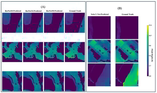
Figure 8. Sampled visualization of predicted test data 256 by 256 tiles for baseline models. (A) CNN-based models. (B) Transformer-based model.

3.2. Scenario 2: Enhanced Model with Terrain-Derived Predictors

In Scenario 2, the inclusion of Topographic Wetness Index (TWI), slope, and curvature alongside the baseline inputs (DTM and flood extent) led to consistent performance improvements across all models. These features enriched the input space with additional hydrologically relevant terrain information, enabling the models to better capture spatial variability in floodwater depth.

ResNet18 emerged as the best-performing model, achieving the lowest RMSE (0.71 ft), and MAE (0.23 ft), as well as the highest SSIM (98.8%) and R-Squared (~94%) scores (Table 7). Relative to the baseline performance, it recorded a 13% reduction in RMSE, 21% decrease in MAE, and moderate gains in SSIM (~1%) and R-Squared (~3%) (Table 8). ResNet34 maintained strong performance overall but showed the least relative improvement, with only modest reductions in RMSE (2.7%) and MAE (11.1%), and marginal increases in SSIM (+0.2%) and R² (+0.2%). While still outperforming ResNet50 in absolute terms (RMSE = 0.72 ft vs. 0.74 ft), the deeper ResNet50 model displayed a greater relative performance gain, with 10.8% lower RMSE, 13.3% lower MAE, and modest increases in SSIM (+0.41%) and R² (+1.87%) scores (Table 7 and Table 8).

Table 7. Evaluation metrics of each model for scenario 2.

Model	RMSE (ft)	MAE (ft)	SSIM (%)	R-Squared (%)	Number of Image Patches
ResNet18	0.71	0.23	98.8	93.5	1185
ResNet34	0.72	0.24	98.7	93.2	1185
ResNet50	0.74	0.26	98.7	92.7	1185
Swin-Unet	1.22	0.47	93.5	81	1185

Table 8. Percentage change in metrics between scenario 1 and scenario 2.

Model	RMSE	MAE	SSIM	R-Squared
ResNet18	−13.41%	−20.69%	+0.51%	+2.75%
ResNet34	−2.70%	−11.11%	+0.20%	+0.22%
ResNet50	−10.84%	−13.33%	+0.41%	+1.87%
Swin-Unet	−28.24%	−30.88%	+1.63%	+24.62%

The Swin-Unet model also benefited from the expanded feature set, even though its absolute performance remained substantially lower than the CNN models (RMSE = 1.22 ft, MAE = 0.47 ft, SSIM = 94%, R-squared = 81%). It showed the largest relative improvement, reducing RMSE and MAE by 28.2% and 30.9%, respectively, and increasing SSIM and R-squared by 1.6% and 24.6%, respectively (Figure 9, Figure 10 and Figure 11).

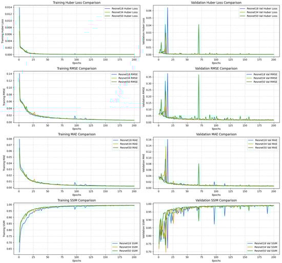
Figure 9. CNN-based models’ training and validation performance plots for scenario 2 enhanced models.

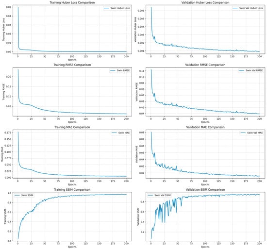
Figure 10. Swin-Unet transformer model training and validation performance plots for scenario 2 enhanced models.

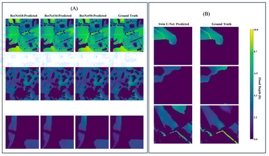
Figure 11. Sampled visualization of predicted test data 256 by 256 tiles for enhanced models. (A) CNN-based models. (B) Transformer-based model.

3.3. Model Generalization over Unseen Catchment Area

To evaluate model generalizability beyond the trained spatial domain, the best-performing model, trained under Scenario 2 using terrain-enhanced inputs, was applied to an unseen catchment area (~534.85 acres) located in Hancheys Store, North Carolina, which was affected by Hurricane Florence in 2018. The best model, ResNet18, predicted a maximum flood depth of approximately 24 ft within this catchment area (Figure 12). However, when compared to its performance on the held-out test set (RMSE = 0.71 ft, MAE = 0.23 ft), a reduction in predictive accuracy was observed, with RMSE increasing to 1.95 ft and MAE to 1.89 ft (Table 9). This corresponds to a 174.6% increase in RMSE and a 721.7% increase in MAE errors (Table 10).

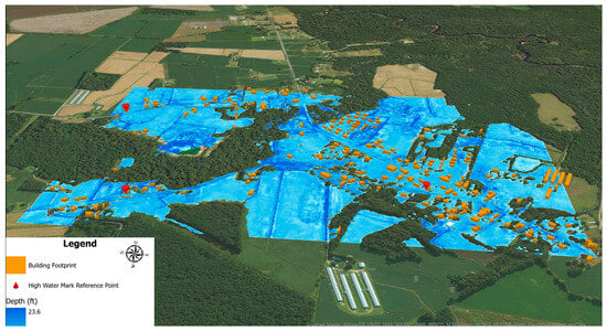
Figure 12. ResNet18 (Enhanced model) floodwater depth prediction map for Hancheys Store, NC-USA.

Table 9. Evaluation metrics of Scenario 2- ResNet18 model on unseen catchment.

Model	RMSE (ft)	MAE (ft)
ResNet18	1.95	1.89

Table 10. Percentage increase in RMSE and MAE for ResNet18 model applied to an unseen catchment, relative to Scenario 2 test performance.

Models	RMSE	MAE
ResNet18	+174.6%	+721.7%

4. Discussion

4.1. Floodwater Depth Prediction with Baseline Extent and DTM

The baseline scenario sought to quantify the predictive capacity of deep learning models when restricted to the two most fundamental drivers of inundation under hydrostatic conditions: (i) the spatial extent of floodwater and (ii) terrain elevation [15,22]. Despite this limited input configuration, the CNN-based models demonstrated strong predictive skill, highlighting the dominant role of terrain gradients in controlling floodwater distribution. The results further confirm that even with limited inputs, CNN architectures can effectively capture the relationship between elevation differences and likely water surface profiles.

Across the tested the architectures, ResNet34 produced the most balanced and accurate predictions, achieving the lowest RMSE (0.74 ft) and MAE (0.27 ft), as well as the highest SSIM (98.5%) and R² (93%). Interestingly, increasing the architecture depth beyond 34 layers did not translate into improved performance. Both ResNet18 and ResNet50 exhibited slightly elevated prediction errors and lower structural similarity scores. This pattern reinforces the notion that deeper networks are not inherently superior, particularly when input features are limited [28]. As model depth increases, the network may become more susceptible to noise or overfitting to small elevation irregularities, as reflected in the higher RMSE values observed for ResNet50. Similar findings have been noted in studies where deeper CNNs provided diminishing returns when the spatial variability of inputs was relatively low or dominated by smooth gradients [33,34].

In contrast, the Swin-Unet transformer model underperformed relative to all three CNN baselines, recording a higher errors (RMSE = 1.7 ft; MAE = 0.68 ft) and much lower structural agreement (SSIM = 92%) and R² (65%). Unlike CNNs, which excel at extracting localized spatial patterns driven by topographic transitions, transformer-based models rely on self-attention mechanisms that typically require more diverse and information-rich inputs. Prior research suggests that transformer architectures perform best when provided with multispectral, multi-temporal, or high-texture imagery that supports learning of long-range dependencies and spatial context [28,29]. In this scenario, where only DTM and a binary flood extent mask were available, the Swin-Unet had limited information on which to base global attention patterns, which likely contributed to its reduced predictive capability compared to CNNs.

Overall, baseline experiment affirms the conceptual validity of estimating floodwater depth from flood extent boundaries and elevation data using deep learning approaches. This is consistent with previous studies that have demonstrated the predictive value and feasibility of learning water surface elevations from inundation patterns and DEM features [3,15,22].

4.2. Floodwater Depth Prediction with Enhanced Terrain Features Under Hydrostatic Conditions

The results from scenario 2 demonstrate that incorporating terrain-derived predictors, specifically slope, curvature, Topographic Wetness Index (TWI), significantly improves the ability of deep learning models to estimate floodwater depth under hydrostatic conditions. These features introduce additional topographic context that directly governs how water accumulates across the urban landscape following flood events. While DTM and flood extent form the basic inputs are needed to constrain water surface elevation, the added terrain descriptors enhance the models’ capacity to differentiate subtle variations in topographic controls that influence local depth variability.

Each terrain variable contributes hydrologically meaningful information. Slope regulates flow resistance and the potential for water accumulation [35]; curvature differentiates convergent zones where water pools from divergent zones where water drains [26]; and TWI identifies areas predisposed to water saturation [14]. By incorporating these predictors, the enhanced models align more closely with the hydrostatic equilibrium assumptions that link local elevation gradients with water surface continuity. As a result, Scenario 2 models produced more accurate and spatially coherent depth estimates compared to those developed using only DTM and flood extent (Table 8).

Among the CNN models, ResNet18 achieved the highest overall accuracy, with the lowest RMSE (0.71 ft) and MAE (0.23 ft), and the highest SSIM (98.8%) and R² (~94%) values. Its improvements over the baseline (13% RMSE reduction; 21% MAE reduction) suggest that shallower architectures can efficiently leverage added terrain complexity without overfitting. ResNet34 and ResNet50 also improved, though by smaller margins, indicating diminishing returns in deeper networks when input variability and training conditions are constrained.

The Swin-Unet model experienced the largest relative gains with the expanded feature set, particularly in RMSE (−28%) and R² (+25%). However, its absolute performance remained substantially lower than that of all CNN models. This pattern supports the conclusion that transformer-based architectures may require richer, more diverse, or multi-temporal inputs to fully capture long-range spatial dependencies. In predominantly static, terrain-driven scenarios, transformers may be underutilized, leading to reduced predictive skill compared to CNNs.

Overall, Scenario 2 confirms that integrating additional terrain descriptors significantly enhances floodwater depth prediction, particularly for CNN architectures that can effectively exploit the finer-scale variability in hydrologic and geomorphic controls. These results highlight the importance of terrain heterogeneity in driving inundation depth patterns and emphasize that carefully selected, physically relevant predictors can substantially improve both accuracy and interpretability of model outputs. In contrast, transformer-based approaches may require more complex and dynamic input configurations to achieve superior performance in flood modeling contexts.

4.3. Generalization over Unseen Catchment

Applying the best model of both scenarios, which is scenario 2 ResNet18 model, to an unseen catchment revealed a notable reduction in predictive accuracy, with RMSE and MAE increasing by 174% and 722%, respectively. These inflated errors are partly a consequence of the extremely limited validation data available in the catchment area, only three high-watermark (HWM) observations were available (Figure 12). With such sparse reference data, a few large residuals can heavily distort RMSE and MAE, which are highly sensitive to outliers under under-sampled conditions [36]. This lack of dense ground truth limits the model’s ability to demonstrate pixel-level accuracy and introduces sampling bias in the evaluation.

Also, the observed degradation may also stem from limited spatial transferability, a known challenge for deep learning models. Deep learning models can become regionally overfit to terrain or hydrologic conditions seen during training, reducing performance in unfamiliar catchments. Such regional overfitting is well documented in geospatial deep learning studies [37,38].

Despite these declines, the best performing model retained the ability to generate spatially consistent and scaled flood depth estimates with relatively good accuracy for practical application in unfamiliar flood-prone regions (Figure 12). It consistently captured the expected scaling of flood depth relative to local terrain structure, suggesting that the learned hydrostatic and terrain-driven relationships remain partly transferable even outside the training region. This is an important characteristic for operational settings, where models often must be deployed beyond their calibration domain.

Overall, the results indicate that while accuracy metrics decline with sparse validation data and domain shift, the model retains practical utility for rapid flood depth estimation in data-limited environments. Such first-pass predictions can support emergency response, risk communication, and post-disaster planning, especially in catchments lacking detailed hydrologic measurements or high-resolution depth observations.

4.4. Limitations and Future Directions

This study encountered key limitations that affect the interpretability, accuracy, and generalizability of the findings.

First, the models’ accuracy were constrained by the resolution and quality of remote sensing inputs. Even with a high-resolution 1-m DTM, errors persisted in densely vegetated areas and where sub-grid features like culverts were poorly captured. These issues may distort and introduce elevation biases into the predictions. Second, the absence of spatially continuous ground-truth flood depth data posed a significant challenge. While flood depth masks were generated using hydrostatic equilibrium assumptions, direct, spatially continuous flood depth observations were unavailable. Even though hydrodynamic models (e.g., LISFLOOD/HECRAS) can offer spatially coherent reference data fidelity, they require site-specific conditions and calibration data that were unavailable across our multi-site sample. In the model generalization experiment, evaluation was based on only three high water mark (HWM) points across a large catchment area (Figure 8), introducing high uncertainty due to spatial under sampling. Furthermore, these HWM points were collected days after the collection of post-event imagery used for flood extent delineation, creating a temporal mismatch. This temporal limitation introduces additional uncertainty, as post-event water recession likely alters actual depth conditions relative to those captured in the input images.

To overcome these limitations and enhance the generalizability and robustness of flood depth prediction frameworks, future research should consider:

(1) Including additional spatial inputs, such as landcover/land use, other terrain indices, and the fusion of Digital Surface Models (DSMs) and DTMs to better capture the complexities of the urban environment.

(2) Using hybrid learning frameworks, where model training and evaluation are guided by physical principles can improve spatial generalization across diverse environments.

(3) Benchmarking newer transformer models (e.g., SegFormer, Mask2Former) alongside CNNs using consistent datasets and training settings.

(4) Generating spatially continuous reference data through advanced hydrostatic simulations (e.g., Rain-on-Grid) to provide better benchmarks for training and evaluation, especially in data-scarce regions. Also, to enhance geographic robustness, future data collection will expand to additional physiographic provinces and sensor modalities (e.g., SAR-derived extents) with domain-balanced sampling.

5. Conclusions

This study demonstrated that deep learning models, particularly the ResNet18 architecture, can reliably estimate post-event floodwater depth using remote sensing and terrain-derived predictors under hydrostatic conditions. Incorporating slope, curvature, and TWI substantially improved model accuracy compared to using DTM and flood extent alone, yielding high structural and statistical agreement with reference depths. Although performance declined when the best model was applied to an unseen peri-urban catchment, due in part to sparse validation data and domain differences, it still produced spatially coherent and physically plausible flood depth patterns. These results highlight both the value and limitations of terrain-informed CNN models for supporting rapid flood assessment in data-scarce environments, and they also suggest that transformer-based models may require richer, multi-temporal inputs to achieve comparable performance.

References

- Mishra, A.; Mukherjee, S.; Merz, B.; Singh, V.P.; Wright, D.B.; Villarini, G.; Paul, S.; Kumar, D.N.; Khedun, C.P.; Niyogi, D.; et al. An Overview of Flood Concepts, Challenges, and Future Directions. J. Hydrol. Eng. 2022, 27, 03122001. [Google Scholar] [CrossRef]
- Blay, J.; Hashemi-Beni, L. Advanced Geo-Data Analytics and AI for 3D Flood Mapping to Protect Built Assets. In ISPRS Annals of the Photogrammetry, Remote Sensing and Spatial Information Sciences; Copernicus Publications: Dubai, United Arab Emirates, 2025. [Google Scholar]
- Blay, J.; Hashemi-Beni, L. Pixels to Insights: Deep Learning for Floodwater Depth Mapping in Settlement Areas; IEEE: Brisbane, Australia, 2025. [Google Scholar]
- Rentschler, J.; Salhab, M.; Jafino, B.A. Flood Exposure and Poverty in 188 Countries. Nat. Commun. 2022, 13, 3527. [Google Scholar] [CrossRef]
- NOAA National Centers for Environmental Information U.S. Billion-Dollar Weather and Climate Disasters. Available online: https://www.ncei.noaa.gov/access/billions/ (accessed on 5 January 2025).
- Hashemi-Beni, L.; Gebrehiwot, A.A. Flood extent mapping: An integrated method using deep learning and region growing using UAV optical data. IEEE J. Sel. Top. Appl. Earth Obs. Remote Sens. 2021, 14, 2127–2135. [Google Scholar] [CrossRef]
- Teng, J.; Penton, D.J.; Ticehurst, C.; Sengupta, A.; Freebairn, A.; Marvanek, S.; Vaze, J.; Gibbs, M.; Streeton, N.; Karim, F.; et al. A Comprehensive Assessment of Floodwater Depth Estimation Models in Semiarid Regions. Water Resour. Res. 2022, 58, e2022WR032031. [Google Scholar] [CrossRef]
- Zhong, P.; Liu, Y.; Zheng, H.; Zhao, J. Detection of Urban Flood Inundation from Traffic Images Using Deep Learning Methods. Water Resour. Manag. 2024, 38, 287–301. [Google Scholar] [CrossRef]
- FEMA. What Building Owners and Tenants Should Know About Urban Flooding. Available online: https://www.fema.gov/sites/default/files/documents/fema_p-2333-mat-report-hurricane-ida-nyc_fact-sheet-1_2023.pdf (accessed on 17 June 2024).
- Alizadeh Kharazi, B.; Behzadan, A.H. Flood Depth Mapping in Street Photos with Image Processing and Deep Neural Networks. Comput. Environ. Urban Syst. 2021, 88, 101628. [Google Scholar] [CrossRef]
- Wu, L.; Liu, Y.; Zhang, J.; Zhang, B.; Wang, Z.; Tong, J.; Li, M.; Zhang, A. Identification of Flood Depth Levels in Urban Waterlogging Disaster Caused by Rainstorm Using a CBAM-Improved ResNet50. Expert Syst. Appl. 2024, 255, 124382. [Google Scholar] [CrossRef]
- Liu, B.; Li, Y.; Feng, X.; Lian, P. BEW-YOLOv8: A Deep Learning Model for Multi-Scene and Multi-Scale Flood Depth Estimation. J. Hydrol. 2024, 645, 132139. [Google Scholar] [CrossRef]
- Du, W.; Qian, M.; He, S.; Xu, L.; Zhang, X.; Huang, M.; Chen, N. An Improved ResNet Method for Urban Flooding Water Depth Estimation from Social Media Images. Measurement 2025, 242, 116114. [Google Scholar] [CrossRef]
- Löwe, R.; Böhm, J.; Jensen, D.G.; Leandro, J.; Rasmussen, S.H. U-FLOOD–Topographic Deep Learning for Predicting Urban Pluvial Flood Water Depth. J. Hydrol. 2021, 603, 126898. [Google Scholar] [CrossRef]
- Gebrehiwot, A.A.; Hashemi-Beni, L. Three-Dimensional Inundation Mapping Using UAV Image Segmentation and Digital Surface Model. Int. J. Geo Inf. 2021, 10, 144. [Google Scholar] [CrossRef]
- Do Lago, C.A.F.; Giacomoni, M.H.; Bentivoglio, R.; Taormina, R.; Gomes, M.N.; Mendiondo, E.M. Generalizing Rapid Flood Predictions to Unseen Urban Catchments with Conditional Generative Adversarial Networks. J. Hydrol. 2023, 618, 129276. [Google Scholar] [CrossRef]
- ESRI ArcGIS Pre-Trained Models. Available online: https://www.arcgis.com/home/item.html?id=a10f46a8071a4318bcc085dae26d7ee4 (accessed on 20 September 2024).
- Fawakherji, M.; Blay, J.; Anokye, M.; Hashemi-Beni, L.; Dorton, J. DeepFlood for Inundated Vegetation High-Resolution Dataset for Accurate Flood Mapping and Segmentation. Sci. Data 2025, 12, 271. [Google Scholar] [CrossRef] [PubMed]
- Blay, J.; Gebregziabher, Y.; Jha, M.K.; Hashemi Beni, L. Inundation2Depth: A Multi-Source Dataset for Floodwater Depth Estimation in Urban Areas. Data Brief 2025, 64, 112347. [Google Scholar] [CrossRef]
- Blay, J.; Agboola, G. Ezprocess Library, version v0.1.0; GitHub: San Francisco, CA, USA, 2025. Available online: https://github.com/Jeffreyblay/ezprocess_library (accessed on 20 September 2025).
- Fawakherji, M.; Anokye, M.; Blay, J.; Hashemi-Beni, L. Multi-Resolution Data Fusion for Resilient Flood Mapping. IEEE Access 2025, 13, 202275–202294. [Google Scholar] [CrossRef]
- Betterle, A.; Salamon, P. Water Depth Estimate and Flood Extent Enhancement for Satellite-Based Inundation Maps. Nat. Hazards Earth Syst. Sci. 2024, 24, 2817–2836. [Google Scholar] [CrossRef]
- Cohen, S.; Raney, A.; Munasinghe, D.; Loftis, D.; Molthan, A.; Bell, J.; Rogers, L.; Galantowicz, J.; Brakenridge, G.R.; Kettner, A.J.; et al. The Floodwater Depth Estimation Tool (FwDET v2.0) for Improved RemoteSensing Analysis of Coastal Flooding. Nat. Hazards Earth Syst. Sci. 2019, 19, 2053–2065. [Google Scholar] [CrossRef]
- Nguyen, H.D.; Dang, D.K.; Nguyen, N.Y.; Pham Van, C.; Van Nguyen, T.T.; Nguyen, Q.-H.; Nguyen, X.L.; Pham, L.T.; Pham, V.T.; Bui, Q.-T. Integration of Machine Learning and Hydrodynamic Modeling to Solve the Extrapolation Problem in Flood Depth Estimation. J. Water Clim. Change 2024, 15, 284–304. [Google Scholar] [CrossRef]
- El Baida, M.; Boushaba, F.; Chourak, M.; Hosni, M. Real-Time Urban Flood Depth Mapping: Convolutional Neural Networks for Pluvial and Fluvial Flood Emulation. Water Resour. Manag. 2024, 38, 4763–4782. [Google Scholar] [CrossRef]
- Burrichter, B.; Hofmann, J.; Koltermann Da Silva, J.; Niemann, A.; Quirmbach, M. A Spatiotemporal Deep Learning Approach for Urban Pluvial Flood Forecasting with Multi-Source Data. Water 2023, 15, 1760. [Google Scholar] [CrossRef]
- Liu, Y.; Wang, H.; Guan, X.; Meng, Y.; Xu, H. Urban Flood Depth Prediction and Visualization Based on the XGBoost-SHAP Model. Water Resour. Manag. 2025, 39, 1353–1375. [Google Scholar] [CrossRef]
- He, K.; Zhang, X.; Ren, S.; Sun, J. Deep Residual Learning for Image Recognition. In Proceedings of the 2016 IEEE Conference on Computer Vision and Pattern Recognition (CVPR), Las Vegas, NV, USA, 27–30 June 2016; IEEE: New York, NY, USA, 2016; pp. 770–778. [Google Scholar]
- Cao, H.; Wang, Y.; Chen, J.; Jiang, D.; Zhang, X.; Tian, Q.; Wang, M. Swin-Unet: Unet-like Pure Transformer for Medical Image Segmentation. In European Conference on Computer Vision; Springer: Cham, Switzerland, 2021. [Google Scholar]
- Liu, Z.; Lin, Y.; Cao, Y.; Hu, H.; Wei, Y.; Zhang, Z.; Lin, S.; Guo, B. Swin Transformer: Hierarchical Vision Transformer Using Shifted Windows. In Proceedings of the 2021 IEEE/CVF International Conference on Computer Vision (ICCV), Montreal, QC, Canada, 10–17 October 2021; IEEE: New York, NY, USA; pp. 9992–10002. [Google Scholar]
- Dang, T.Q.; Tran, B.H.; Le, Q.N.; Dang, T.D.; Tanim, A.H.; Pham, Q.B.; Bui, V.H.; Mai, S.T.; Thanh, P.N.; Anh, D.T. Application of Machine Learning-Based Surrogate Models for Urban Flood Depth Modeling in Ho Chi Minh City, Vietnam. Appl. Soft Comput. 2024, 150, 111031. [Google Scholar] [CrossRef]
- Museru, M.L.; Nazari, R.; Giglou, A.N.; Opare, K.; Karimi, M. Advancing Flood Damage Modeling for Coastal Alabama Residential Properties: A Multivariable Machine Learning Approach. Sci. Total Environ. 2024, 907, 167872. [Google Scholar] [CrossRef] [PubMed]
- Luo, W.; Li, Y.; Urtasun, R.; Zemel, R. Understanding the Effective Receptive Field in Deep Convolutional Neural Networks. In Advances in Neural Information Processing Systems; MIT Press: Cambridge, MA, USA, 2016. [Google Scholar]
- Rahaman, N.; Baratin, A.; Arpit, D.; Draxler, F.; Lin, M.; Hamprecht, F.A.; Bengio, Y.; Courville, A. On the Spectral Bias of Neural Networks. Proc. Mach. Learn. Res. 2019, 97, 5301–5310. [Google Scholar]
- He, J.; Zhang, L.; Xiao, T.; Wang, H.; Luo, H. Deep Learning Enables Super-Resolution Hydrodynamic Flooding Process Modeling under Spatiotemporally Varying Rainstorms. Water Res. 2023, 239, 120057. [Google Scholar] [CrossRef]
- Elharrouss, O.; Mahmood, Y.; Bechqito, Y.; Serhani, M.A.; Badidi, E.; Riffi, J.; Tairi, H. Loss Functions in Deep Learning: A Comprehensive Review. arXiv 2025, arXiv:2504. [Google Scholar] [CrossRef]
- Baste, S.; Klotz, D.; Espinoza, E.A.; Bardossy, A.; Loritz, R. Unveiling the Limits of Deep Learning Models in Hydrological Extrapolation Tasks. Hydrol. Earth Syst. Sci. 2025, 29, 5871–5891. [Google Scholar] [CrossRef]
- Seleem, O.; Ayzel, G.; Bronstert, A.; Heistermann, M. Transferability of Data-Driven Models to Predict Urban Pluvial Flood Water Depth in Berlin, Germany. Nat. Hazards Earth Syst. Sci. 2023, 23, 809–822. [Google Scholar] [CrossRef]
Disclaimer/Publisher’s Note: The statements, opinions and data contained in all publications are solely those of the individual author(s) and contributor(s) and not of MDPI and/or the editor(s). MDPI and/or the editor(s) disclaim responsibility for any injury to people or property resulting from any ideas, methods, instructions or products referred to in the content. |
© 2025 by the authors. Licensee MDPI, Basel, Switzerland. This article is an open access article distributed under the terms and conditions of the Creative Commons Attribution (CC BY) license.