RSSRGAN: A Residual Separable Generative Adversarial Network for Remote Sensing Image Super-Resolution Reconstruction

Highlights

What are the main findings?

• RSSRGAN improves residual dense networks by introducing depthwise separable convolutions and dual PatchGAN discriminators, boosting training speed by 9.89% and stabilizing metrics, a key breakthrough over traditional GAN-based super-resolution models.
• Integrating Charbonnier-MSE mixed content loss and joint perceptual loss, the model achieves notable metric gains: 18.8% higher PSNR, 8.0% higher SSIM, 3.6% lower MSE, and 13.6% higher PI vs. the widely used SRGAN in the remote sensing field (this paper uses satellite-specific SRGAN for comparison).

What are the implications of the main findings?

• The innovative design balances perceptual quality and pixel accuracy, effectively enhancing details, colors, and brightness of remote sensing images, even in low-light/narrow-field scenarios where conventional models fail.
• With reduced computation from architectural and loss optimizations, it integrates seamlessly into remote sensing pipelines and enables potential edge deployment, addressing hardware limitations in real-world remote sensing tasks.

Abstract

With the advancement of remote sensing technology, high-resolution images are widely used in the field of computer vision. However, image quality is often degraded due to hardware limitations and environmental interference. This paper proposes a Residual Separable Super-Resolution Reconstruction Generative Adversarial Network (RSSRGAN) for remote sensing image super-resolution. The model aims to enhance the resolution and edge information of low-resolution images without hardware improvements. The main contributions include (1) designing an optimized generator network by improving the residual dense network and introducing depthwise separable convolutions to remove BN layers, thereby increasing training efficiency—two PatchGAN discriminators are designed to enhance multi-scale detail capture—and (2) introducing content loss and joint perceptual loss on top of adversarial loss to improve global feature representation. Experimental results show that compared to the widely used SRGAN model in remote sensing (exemplified by the satellite-specific SRGAN in this study), this model improves PSNR by approximately 18.8%, SSIM by 8.0%, reduces MSE by 3.6%, and enhances the PI metric by 13.6%. It effectively enhances object information, color, and brightness in images, making it more suitable for remote sensing image super-resolution.

1. Introduction

Remote sensing technology involves acquiring data about target objects without direct contact, by receiving and recording electromagnetic waves reflected or emitted from the target via sensors on platforms (e.g., drones, satellites). This information is then processed and interpreted to obtain data related to the target’s environment, spatial distribution, and changing characteristics. The core value of remote sensing technology lies in its ability to collect target information quickly, periodically, and over large areas, making it widely applicable in resource exploration, environmental monitoring, urban planning, and more [1]. It can be said that the emergence of remote sensing technology has significantly expanded the application scope of high-resolution digital images in various fields.

However, the acquisition of remote sensing images is often affected by factors such as hardware performance limitations, motion blur, atmospheric disturbance, and electromagnetic interference, leading to degraded image quality. To address the problem of low-resolution remote sensing images, Dong et al. introduced Convolutional Neural Networks (CNNs) into the super-resolution field [2]. Their Super-Resolution Convolutional Neural Network (SRCNN) utilized deep learning to convert low-resolution images into high-resolution ones, breaking the limitations of traditional methods and laying the foundation for subsequent deep learning-based super-resolution models. However, SRCNN requires extensive data and computational resources for training and exhibits mediocre real-time performance. The Generative Adversarial Networks (GANs) proposed by Goodfellow et al. [3] represented another major advancement. GANs consist of a generator and a discriminator in a competitive framework, capable of generating highly realistic data. The Super-Resolution Generative Adversarial Network (SRGAN) [4] applied GAN principles to super-resolution, generating visually more realistic high-resolution images. Nevertheless, SRGAN still faces challenges in training complexity, spatial feature processing, edge sharpness, and model stability. The Enhanced Super-Resolution Generative Adversarial Network (ESRGAN) [5], building upon SRGAN, introduced a deeper network architecture, residual and dense connections, and innovative loss functions to improve image quality. Similar GAN-based works include the Conditional Generative Adversarial Network (CGAN) [6], Deep Convolutional Generative Adversarial Network (DCGAN) [7], and Cycle-Consistent Generative Adversarial Network (CycleGAN) [8]. Although these models achieved improved accuracy, their increased complexity demands more computational resources, and their effectiveness in remote sensing applications remains to be fully evaluated.

To address the above challenges, this paper proposes a Residual Separable Super-Resolution Reconstruction Generative Adversarial Network (RSSRGAN) for remote sensing image super-resolution. Firstly, we designed an optimized generator network by improving the Residual Dense Network and introducing Depthwise Separable Convolutions to remove BN layers, significantly improving training efficiency. Secondly, we designed two PatchGAN discriminators to enhance multi-scale detail capture and improve the authenticity of local details. Finally, we introduced content loss and perceptual loss to optimize the loss function, enhancing model stability and providing more comprehensive, multi-scale feature constraints.

These modules can effectively improve training stability and speed. Furthermore, while maintaining the advantage of high perceptual quality from SRGAN, they effectively improve metrics such as PSNR and SSIM. Ultimately, the improved model can generate super-resolved images with extremely rich and realistic local details, featuring both sharp edges and correct semantics. Our main contributions are summarized as follows:

• Training speed is increased by approximately 9.89%, and the average standard deviation of stabilized metrics is 80% of the baseline, alleviating the issues of high computational cost and training instability in SRGAN to some extent.
• Compared with the widely used SRGAN in the remote sensing field (this paper uses satellite-specific SRGAN for comparison), the PSNR improved by 18.8%, SSIM improved by 8.0%, MSE decreased by 3.6%, and PI improved by 13.6%, continuing the advantage of high perceptual quality from SRGAN while also improving other pixel-level accuracy metrics.
• Superior details with reduced local inconsistent artifacts, exhibiting excellent performance in enhancing ground object information, color richness, and brightness.

2. Related Works

2.1. Traditional Non-Deep Learning Methods

The core idea of traditional super-resolution methods is to utilize the image’s own prior knowledge or an example library to reconstruct a high-resolution image from N low-resolution images. These methods are simple to implement and computationally efficient, performing well in simple super-resolution tasks and laying the groundwork for subsequent deep learning methods.

Traditional non-deep learning methods can be broadly categorized into interpolation-based methods, reconstruction-based methods, and traditional machine learning methods. Interpolation methods are based on the assumption that “pixel values change smoothly in their neighborhood,” inferring unknown high-resolution pixel values by calculating the weighted average of known surrounding pixels. Interpolation methods are very fast and simple but can only perform smooth enlargement and cannot recover high-frequency details [9]. Representative algorithms include Bilinear Interpolation and Bicubic Interpolation. Reconstruction methods are more complex; their principle assumes that multiple observed LR images(Low-Resolution image) are generated from the same HR image(High-Resolution image) after undergoing geometric deformation, blurring, downsampling, and noise addition. The goal is to find an HR image that, after passing through the aforementioned degradation model, can simulate all observed LR images as closely as possible [10]. Although reconstruction methods perform better than interpolation methods, they also have limitations such as high input requirements and limited magnification factors. Representative algorithms include Iterative Back Projection (IBP) and Projection Onto Convex Sets (POCS). The core idea of traditional machine learning methods is to learn the mapping relationship between LR and HR image patches from external examples. Compared to the previous two methods, it achieves the best results but also suffers from issues like unnatural details and high computational complexity. Representative traditional machine learning algorithms include Neighbor Embedding and Sparse Coding.

In summary, traditional non-deep learning methods are computationally efficient and simple to implement and were once widely used. However, their performance is limited by handcrafted models and prior knowledge, which are often not powerful enough to perfectly describe the complex structure and detailed textures of natural images, usually resulting in blurry outputs with lost high-frequency details, making the super-resolution results less than ideal.

2.2. Non-GAN Deep Learning Methods

As mentioned in the introduction, Dong et al. [2] pioneered the use of convolutional neural networks for super-resolution. The core idea of deep learning-based image super-resolution is to use neural networks (DNNs) [11] to directly learn the complex nonlinear mapping relationship between low- and high-resolution image pairs from massive amounts of data. Compared to traditional non-deep learning methods, it successfully shifted from “model-driven” to “data-driven,” allowing the network to automatically learn optimal image prior knowledge from data. The hierarchical features learned by the network in its deep layers are much more powerful than handcrafted features, enabling better capture of semantic information and textural details. These methods often pursue higher fidelity and perform exceptionally well on objective metrics like PSNR and SSIM.

Non-GAN deep learning methods were initiated by SRCNN, which first demonstrated the great potential of CNNs in super-resolution tasks. SRCNN has a simple structure and a small receptive field, requires upsampling the LR image first, and has low computational efficiency. With the proposal of ResNet [12], network depth was greatly increased, represented by models like VDSR [13]. These models not only have deeper networks and larger receptive fields but also optimize the learning objective to learn the residual map rather than directly learning the HR image, simplifying the learning goal and significantly accelerating training. To perform upsampling efficiently, models such as ESPCN [14] and EDSR [15] emerged. ESPCN moves most computations to the LR space and finally reorganizes the channel number into spatial resolution through a PixelShuffle operation. This method is far more computationally efficient than previous methods that computed after upsampling. EDSR removes BN layers and constructs very wide and deep networks by stacking residual blocks and increasing the number of filters. This approach not only effectively improves computational efficiency but also greatly enhances PSNR metrics. In subsequent developments, models incorporating channel attention, such as RCAN [16] and RNAN [17], appeared. These methods allow the network to utilize the model more intelligently, making them suitable for recovering global structures. There are also models that introduce Vision Transformers [18] into image restoration, such as SWINIR [19]. It introduces the global modeling capability of Transformers into pixel-level restoration tasks through local window attention and a sliding window mechanism, significantly improving performance while reducing parameters and computation.

In summary, non-GAN deep learning methods pursue extreme fidelity, excel in objective metrics like PSNR and SSIM, and are essential for image super-resolution tasks requiring pixel-level accuracy, such as medical imaging and microscope images. However, overemphasizing pixel-accurate objective metrics while neglecting subjective metrics can lead to mediocre performance in super-resolution tasks where human visual perception is highly important.

2.3. Generative Adversarial Network-Based Methods

The previously mentioned non-GAN deep learning methods focus more on pixel-level error, pursuing higher PSNR, SSIM, and other objective metrics. However, this can result in overly smooth outputs that are not visually realistic enough. The introduction of Generative Adversarial Networks opened up new possibilities for super-resolution. It introduces a discriminator to compete with the generator; both learn continuously—the generator strives to generate more realistic images to “fool” the discriminator, while the discriminator strives to improve its ability to distinguish between real and generated images. This process forces the generator to learn the data distribution on the natural image manifold, thereby generating images with more realistic textural details.

The performance of models incorporating GANs improved qualitatively, which is inseparable from their various loss function designs and network architecture innovations. Loss functions include adversarial loss that encourages the generator output to match the real image distribution, pixel-level loss that ensures the overall structure and color of the generated image are consistent with the target, style loss that helps match the texture style of real images, etc. In terms of network architecture innovation, powerful regression networks like EDSR and RRDB are typically used as the backbone to ensure strong mapping capabilities. SRGAN was the first work to apply GANs to super-resolution, generating detail-rich textures for the first time, which was visually impressive. It can be said that SRGAN is a major milestone in the field of perceptual super-resolution. However, SRGAN sometimes produces unnatural artifacts, and its objective metrics like PSNR are relatively low. Building on this, an enhanced version, ESRGAN, emerged. ESRGAN removes BN layers to improve generative capability. It also optimizes the discriminator into a relativistic discriminator, changing the judgment from “absolute real or fake” to “relatively real or fake,” making training more stable. Images generated by ESRGAN have sharper and more natural textures, with significantly improved perceptual quality, making it one of the most popular GAN-based models today. In 2021, Real-ESRGAN [20] extended ESRGAN’s capabilities to real-world images. It simulates more complex degradation processes during training data synthesis, enabling the model to handle more diverse, complex, and unknown degradations in the real world. Furthermore, the discriminator is optimized to provide pixel-level gradient feedback, effectively repairing local artifacts.

For remote sensing image tasks, several derived models have emerged, including SAGAN [21], an improved SRGAN model with multi-scale residual structures targeting remote sensing imagery [22], and an enhanced SRGAN model specifically designed for satellite images. SAGAN employs Instance Normalization, which is more suitable for image generation tasks [23]. It eliminates instance-specific contrast information, thereby improving the quality of generated images and training stability. Additionally, this model incorporates attention mechanisms and optimizes the loss function to enhance the generator structure, significantly improving texture reconstruction effects and optimizing global feature fusion. It is currently one of the superior GAN-based models for remote sensing images, though its perceptual quality still has room for improvement. The multi-scale residual SRGAN utilizes a multi-scale residual architecture and an improved loss function, achieving notable gains in PSNR. However, its improvements in SSIM and perceptual quality metrics remain limited. The satellite-specific SRGAN adopts a residual network design tailored for single satellite remote sensing images. This model serves as the baseline in our study.

In summary, images generated by GANs are more aligned with human subjective perception, easily generating more realistic textures, and far surpass other methods in visual effect. Additionally, during training, these models can deduce and reconstruct lost information rather than simply performing smooth interpolation. However, existing GAN-based image super-resolution models also have drawbacks. A prominent issue is that higher perceptual quality often implies lower fidelity, so these models generally perform modestly on objective metrics like PSNR and SSIM. Furthermore, GAN training is not very stable and incurs high computational costs, which are problems that need to be addressed.

3. The Method

3.1. Generator and Discriminator Networks

Based on the analysis and research of separable convolutional sparse residual networks, we designed a generator network model. Different from the classical SRGAN, we removed the BN layers to ensure model stability and improve generalization ability. Simultaneously, removing BN layers also reduces computational load. To further reduce computational load, we employed depthwise separable convolution kernels. The final generator network structure is shown in Figure 1. The generator consists of convolutional layers and sparse residual dense network layers to achieve image super-resolution reconstruction.

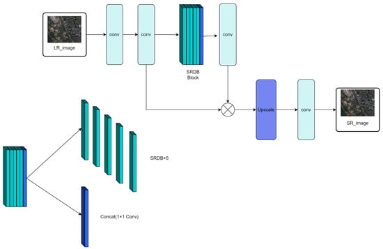
Figure 1. Generator Network Structure. Where SRDB is Supervised Residual Dense Block.

A fundamental limitation of a single global discriminator is its failure to penalize localized distortions effectively, as minor artifacts are averaged out over the entire image, compromising high-fidelity reconstruction in local regions. To solve this problem, we use two structurally identical discriminators, Dx and Dy, to distinguish between real and fake low-resolution and high-resolution images, respectively. The former acts on the entire image, judging whether the image as a whole is real and natural. The latter randomly crops multiple small patches from the SR or HR image, judging whether the texture of each local region of the image is real. To enhance texture and edge details and improve the value of remote sensing images, as shown in Figure 2, our designed discriminator contains 8 convolutional layers, each followed by batch normalization, and uses the activation function from [24] to reduce feature map size and avoid gradient vanishing, thereby improving training stability. Additionally, we introduce connection layers to fuse features and capture contextual relationships. Finally, a Sigmoid function is used to convert the output into a probability prediction, providing reliable results for remote sensing image super-resolution.

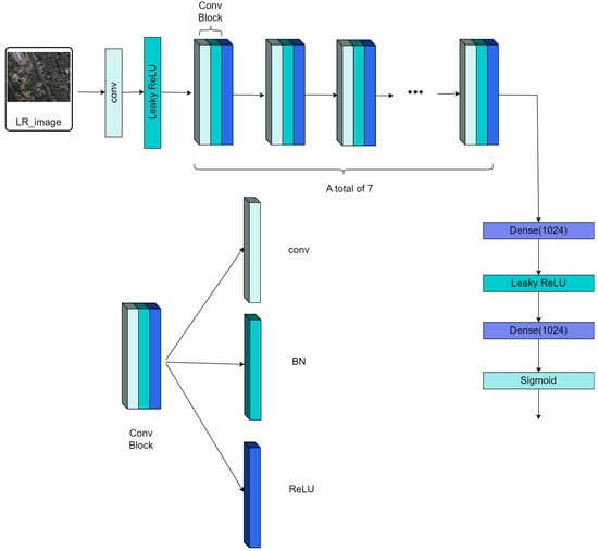
Figure 2. Discriminator Network Architecture. Where Leaky ReLU is A teal-colored rectangle representing the activation function used after convolutional or dense layers to introduce non-linearity, Dense is A purple-colored rectangle representing a fully-connected layer, with the number (e.g., 1024) indicating the number of neurons and Sigmoid is A light green-colored rectangle representing the sigmoid activation function, typically used in the output layer for tasks like probability estimation.

3.2. Depthwise Separable Convolution

To further reduce computational load, based on the SRGAN framework, this paper further proposes the use of depthwise separable convolution, replacing the original 3 × 3 convolutional layer with a pointwise convolution and using 3 × 1 and 1 × 3 convolutional layers. Depthwise separable convolution reduces the number of parameters to 1/L + 1/C² of that in standard convolution, and its parameter ratio to conventional convolution is expressed by the following equation.

$$R={\displaystyle \frac{{\mathrm{Params}}_{\mathrm{dsc}}}{{\mathrm{Params}}_{\mathrm{std}}}}={\displaystyle \frac{1}{L}}+{\displaystyle \frac{1}{C^2}}$$

(1)

where C represents the convolution kernel length and width, ${\mathrm{P}\mathrm{a}\mathrm{r}\mathrm{a}\mathrm{m}\mathrm{s}}_{\mathrm{d}\mathrm{s}\mathrm{c}}$ represents the parameters of depthwise separable convolution, ${Params}_{std}$ represents the parameters of standard convolution and L represents the convolution kernel height.

Furthermore, as shown in the following equation, the ratio of Floating-Point Operations (FLOPs) between the two convolution methods also indicates that the FLOPs of depthwise separable convolution are significantly lower.

$${\displaystyle \frac{F_{\mathrm{depth}\text{-}\mathrm{sep}}}{F_{\mathrm{standard}}}}\approx {\displaystyle \frac{1}{C_{\mathrm{out}}}}+{\displaystyle \frac{1}{K^2}}$$

(2)

where ${\mathrm{C}}_{\mathit{out}}$ is the number of output channels, and K is the convolution kernel size.

Figure 3 and Figure 4 illustrate schematic diagrams of conventional convolution and depthwise separable convolution, respectively. It can be observed that the parameter count of the depthwise separable convolution model is significantly lower than that of the conventional convolution model.

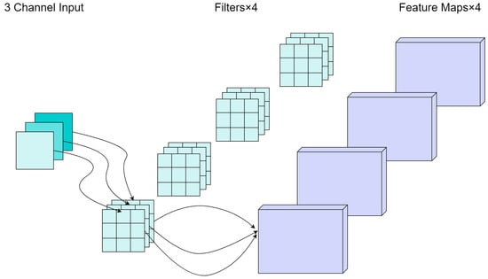
Figure 3. The schematic of conventional convolution.

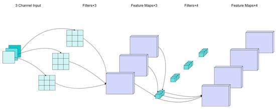
Figure 4. The schematic of depthwise convolution.

3.3. Training

The loss function is crucial in network design and optimization, determining the learning objective and performance. Our total loss function incorporates four types of loss: adversarial loss, Charbonnier + MSE mixed loss, VGG perceptual loss, and TV regularization loss.

3.3.1. Adversarial Loss Function

The core task of the adversarial loss is to enhance the realism of the image, avoid generating blurry and unnatural visuals, encourage the generator to produce more realistic images, and force the discriminator to improve its discrimination ability, as shown in Equation (3):

$$l_{\mathrm{Gen}}^{\mathrm{SR}}={\displaystyle \sum _{n=1}^N-}\log D_{{\theta }_D}\left(G_{{\theta }_G}{I}^{\mathrm{LR}}\right)$$

(3)

where D is the discriminator, G is the generator, LR represents the low-resolution image, and θ represents the generator parameters.

3.3.2. Content Loss Function

This measures the pixel-level difference between the generated image and the original high-resolution image. Its core purpose is to ensure content accuracy and avoid generating content that deviates from the original image. Image super-resolution tasks typically use MSE as the loss function, but pure MSE is very sensitive to outliers, allowing a few large errors to dominate gradient updates, leading to overly smooth reconstructions or artifacts. The MSE formula is shown in Equation (4):

$$L_{\mathrm{MSE}}={\displaystyle \frac{1}{N}}{\displaystyle \sum _{i=1}^N{(y_i-{\widehat{y}}_i)}^2}$$

(4)

where N is the number of samples in the batch, $y_i$ is the true value for the i-th sample and ${\widehat{y}}_i$ is the predicted value for the i-th sample.

As this equation shows, the squared term amplifies the impact of errors. The Charbonnier loss is a smooth approximation of the L1 loss, introduced with an epsilon ($\mathsf{ϵ}$) parameter to avoid gradient explosion, making it more robust to outliers [25]. Its formula is shown in Equation (5):

$$L_{\mathrm{Charbonnier}}=\sqrt{{\left(y_i-{\widehat{y}}_i\right)}^2+{ϵ}^2}$$

(5)

where $ϵ$ is a very small constant to avoid the square root being zero. This model is overall smoother than MSE, making training more stable. Therefore, we propose a hybrid form of Charbonnier loss (60%) + MSE (40%), which is more suitable for handling outliers. The improved content loss function is as follows:

$$L_{\mathrm{content}}=\alpha \cdot L_{\mathrm{MSE}}+(1-\alpha )\cdot L_{\mathrm{Charbonnier}}+\beta \cdot L_{\mathrm{gradient}}$$

(6)

where α and β are parameters. Based on experimental results, α = 0.4 and β = 0.2 yield the best results. $L_{\mathit{gradient}}$ is the gradient loss function, with the formula as follows:

$$L_{\mathrm{gradient}}={\displaystyle \frac{1}{N}}{\displaystyle \sum _{i=1}^N\Vert \nabla y_i-\nabla {\widehat{y}}_i{\Vert }_1}$$

(7)

where $y_i$ represents the i-th real image, ${\widehat{y}}_i$ represents the i-th predicted image and ∇ is the gradient operator.

3.3.3. Perceptual Loss Function

We propose an innovative perceptual loss function to reduce subtle differences in content and structure between the generated image and the real high-resolution image. The proposed perceptual loss is based on the high-level feature maps of a deep convolutional network, focusing on semantic and visual perception similarity, and is widely used in GAN tasks such as image super-resolution and style transfer.

To restore and enhance high-frequency details in super-resolved images and improve image quality and perception, we introduce a joint perceptual loss that balances high-frequency and low-frequency features. By adjusting weights, flexible control over different features is achieved, generating more natural and realistic super-resolution images. Research shows that sparse features aid feature selection, but in super-resolution reconstruction, the supervisory effect of sparse features is weaker because they compress information and limit the contribution to details and structure. To address this, we choose to use features before activation rather than after activation when calculating the perceptual loss. These uncompressed features are richer and more diverse, containing more original data information, providing stronger supervision, and helping the network better learn and restore image details and structure. The improved perceptual loss function is shown in Equation (8):

$$l_{\mathrm{VGG}}^{\mathrm{SR}}=\alpha \times {\mathrm{VGG}}_{22}+\beta \times {\mathrm{VGG}}_{54}$$

(8)

where α and β are hyperparameters and ${VGG}_{22},{VGG}_{54}$ represent the feature maps extracted from the 22nd layer and 54th layer of the pre-trained VGG-19 network. Based on cross-validation experimental results, this paper sets α = 0.01 and β = 1. The final improved loss function is shown in Equation (9):

$$l^{SR}=l_{VGG}^{SR}+{10}^{-2}{l}_{MSE}^{SR}+{10}^{-3}{l}_{GEN}^{SR}$$

(9)

where $l^{SR}$ is the total loss for Super-Resolution, $l_{VGG}^{SR}$ is VGG loss, $l_{MSE}^{SR}$ is the Mean Squared Error loss and $l_{GEN}^{SR}$ is the adversarial loss from the generator.

3.3.4. Total Variation Loss Function

It can reduce noise and artifacts in the generated image by smoothing pixel variations, making the visuals more natural. In our experiments, we introduce TV loss to suppress noise and artifacts in the generated image while enhancing edge smoothness and structural consistency. TV loss constrains the spatial smoothness of the generated image by minimizing the magnitude of the local image gradient [26]. Its definition in continuous mathematics is shown in Equation (10):

$${\mathcal{L}}_{TV}={\displaystyle {\int }_{\mathsf{\Omega }}\left(\left|{\nabla }_{x}I\right|+\left|{\nabla }_{y}I\right|\right)}dxdy$$

(10)

where ∇_x and ∇_y represent the gradient operators of the image I in the horizontal and vertical directions, respectively, and Ω represents the domain of the image. The formula shown in (10) is suitable for ideal continuous images, whereas in practical applications, the following formula is typically used:

$${\mathcal{L}}_{TV}={\displaystyle \sum _{i,j}\left(\left|x_{i+1,j}-x_{i,j}\right|+\left|x_{i,j+1}-x_{i,j}\right|\right)}$$

(11)

where x_i,j represents the pixel value at row i and column j of the image. Equation (11) is equivalent to Equation (10) but is more suitable for computer program implementation and calculation, measuring the overall fluctuation degree of the image by calculating the sum of absolute differences of pixels in the horizontal and vertical directions.

4. Experiments

4.1. Datasets

Regarding datasets, considering the model’s adaptability and effectiveness in different environments, we prepared multiple datasets. The first dataset is the UAVDT Dataset, released in 2018 by research teams from the National University of Singapore and Peking University. It aims to advance three key tasks in UAV applications: object detection, single object tracking, and multi-object tracking. It is suitable for computer vision research, machine learning, and artificial intelligence, and can be used for the development, optimization, training, and validation of related algorithms. Its characteristics lie in the asymmetry of data distribution, such as significant differences in target scale, perspective, and scenes, forming a sharp contrast with conventional remote sensing datasets (e.g., DOTA, DIOR). This dataset contains approximately 80,000 frames. The image data mainly comes from UAV flight records in different urban locations, covering various typical environments such as squares, main roads, toll stations, highways, and road intersections, offering broad applicability.

The second dataset is the CODrone UAV dataset released in 2025 by the MAC Laboratory of Xiamen University. It features high-resolution image acquisition, a rich target category system, multi-angle and multi-altitude flight data, and collection under multiple environments and lighting conditions, comprehensively covering real flight environments. It possesses high challenge and diversity and can be used to promote the further development of UAV visual perception technology in real environments. The images are 3840 × 2160 4K high-definition pixels, containing 10,004 images. Data collection spans dawn, day, dusk, and night, across multiple cities, towns, ports, and industrial areas. This dataset can effectively reflect the model’s adaptability under different lighting environments.

The third dataset is VisDrone. This is a well-known drone perspective object detection dataset released by the Machine Learning and Data Mining Laboratory of Tianjin University. Based on the original VisDrone2019-DET dataset, it has been improved to focus more on low-altitude drone images. The targets include small objects such as cars, buildings, and people, effectively reflecting the model’s ability to reconstruct details.

In order to obtain a model that is more capable of handling real and complex environments, less prone to overfitting, and more robust, we combined the datasets mentioned above. To address the domain shift problem that often arises with mixed datasets, we have implemented corresponding measures: all images in the dataset are resized to a uniform resolution of 1024 × 512 pixels, and histogram matching preprocessing is applied to reduce distribution discrepancies. Furthermore, the dual-discriminator model mentioned earlier, which excels in handling details and enhancing cross-scale feature capture, also helps mitigate this problem to some extent. It was divided into training, validation, and test sets in an 8:1:1 ratio. These subsets were used for network training, parameter adjustment during the learning phase, and model evaluation, respectively.

Figure 5 shows part of the mixed dataset images.

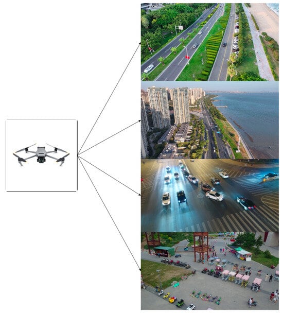
Figure 5. Part of the mixed dataset images.

4.2. Evaluation Metrics

Quantitative analysis provides an objective method for evaluating super-resolution algorithm performance. The metrics used in this paper include: Peak Signal-to-Noise Ratio (PSNR), Structural Similarity Index (SSIM), Mean Squared Error (MSE), Perceptual Index (PI), Discriminator Loss, Generator Loss, Number of Parameters, and FLOPs.

4.2.1. PSNR (Peak Signal-to-Noise Ratio)

The core idea of PSNR is based on MSE, representing the ratio between the “maximum possible signal power” and the “corrupting noise power.” It can be understood as the proportion of effective information to noise in the image, measuring the pixel-level error between the reconstructed image and the real image, in units of dB. A higher value indicates less distortion. Its formula is shown in Equation (12):

$$\mathrm{PSNR}=10\cdot {\log }_{10}\left({\displaystyle \frac{{\mathrm{MAX}}_I^2}{\mathrm{MSE}}}\right)$$

(12)

where ${\mathrm{MAX}}_I$ is the maximum possible pixel value of the image.

4.2.2. MSE (Mean Squared Error)

The core idea of MSE is to calculate the average of the squared differences between corresponding pixel values in two images. It only cares about the numerical difference in pixel values and does not consider the structural information of the image content at all, directly reflecting numerical differences. However, this metric correlates poorly with human subjective visual perception.

$$\mathrm{MSE}={\displaystyle \frac{1}{MN}} {\displaystyle \sum }_{i=1}^M{\displaystyle \sum }_{j=1}^N{[I(i,j)-K(i,j)]}^2$$

(13)

where I is the reference image, K is the image to be evaluated, and MN is the resolution of the image.

4.2.3. SSIM (Structural Similarity Index)

The core idea of SSIM is that the human eye primarily extracts structural information from images [27]. It compares two images from three dimensions: luminance, contrast, and structure, making it closer to human visual perception than PSNR.

$$\mathrm{SSIM}(x,y)={\displaystyle \frac{\left(2{\mu }_x{\mu }_y+C_1\right)\left(2{\sigma }_{xy}+C_2\right)}{\left({\mu }_x^2+{\mu }_y^2+C_1\right)\left({\sigma }_x^2+{\sigma }_y^2+C_2\right)}}$$

(14)

where ${\mu }_x{, \mu }_y$ are the means of images x and y, ${\sigma }_x^2{, \sigma }_y^2$ are the variances, ${\sigma }_{\mathit{xy}}$ is the covariance, and $C_1{, C}_2$ are constants to avoid division by zero.

4.2.4. PI (Perceptual Index)

It utilizes a pre-trained CNN (e.g., VGG) to extract deep features, calculates the distance in feature space, captures semantic-level differences, and is highly correlated with human subjective scores.

$$PI={\displaystyle \frac{1}{2}}((10-Ma)+NIQE)$$

(15)

where Ma is the score calculated by the BLIINDS-II model [28], and NIQE is the score calculated by the NIQE model.

4.2.5. Dloss (Discriminator Loss)

Dloss is the optimization objective of the discriminator. For real data, the probability output by the discriminator should be as large as possible. For generated data, the probability output should be as small as possible. Its formula is as follows:

$$L_D=L_{\mathrm{Discriminator}}={\mathbb{E}}_{x~p_{\mathrm{data}}(x)}[\log D(x)]+{\mathbb{E}}_{z~p_z(z)}[\log (1-D(G(z)))]$$

(16)

where $\mathbb{E}$ is the expectation value, x~$p_{\mathit{data}}$ is a sample from the real data distribution $p_{\mathit{data}}$, z~$p_z$ is a sample from the prior noise distribution (e.g., standard normal distribution), D(x) is the discriminator’s judgment result for the real sample x, a scalar between 0 and 1, representing the probability that the discriminator considers x to be real data. G(z) is the fake sample generated by the generator from noise z. D(G(z)) is the discriminator’s judgment result for the generated sample G(z), representing the probability that the discriminator considers this fake sample to be real.

4.2.6. Gloss (Generator Loss)

Gloss is the optimization objective of the generator, aiming to improve the generator’s ability to “fool” the discriminator. Its formula is as follows:

$$L_G=L_{Generator}={\mathbb{E}}_{z~p_z(z)}[\log (1-D(G(z)))]$$

(17)

The explanations for this equation are similar to those for Equation (16).

4.2.7. Number of Parameters, FLOPs and Inference Speed

Parameters refer to the total number of weights and biases in the model that need to be learned and stored. It determines the model size. In the case of depthwise separable convolution, its formula is as follows:

$${\mathrm{Params}}_{\mathrm{dsc}}=C\times C\times A\times X\times Y+A\times L\times X\times Y$$

(18)

where A is the input channels, C refers to the number of input and output channels and X × Y is input size.

FLOPs measure the computational cost required to perform one forward pass (inference). In the case of depthwise separable convolution, its formula is as follows:

$$F_{\mathrm{depth}\text{-}\mathrm{sep}}=F_{\mathrm{depthwise}}+F_{\mathrm{pointwise}}=2\times C_{\mathrm{in}}\times H_{\mathrm{out}}\times W_{\mathrm{out}}\times (K^2+C_{\mathrm{out}})$$

(19)

where $F_{\mathrm{d}\mathrm{e}\mathrm{p}\mathrm{t}\mathrm{h}\mathrm{w}\mathrm{i}\mathrm{s}\mathrm{e}}$ is the computational cost of the depthwise convolution stage, $F_{\mathrm{p}\mathrm{o}\mathrm{i}\mathrm{n}\mathrm{t}\mathrm{w}\mathrm{i}\mathrm{s}\mathrm{e}}$ is the computational cost of the pointwise convolution stage, $C_{in}$ is the number of channels in the input feature map, $C_{out}$ is the number of channels in the output feature map, $H_{\mathit{out}}$ and $W_{\mathit{out}}$ are the height and width of the output feature map.

Both are important metrics for designing efficient neural networks, reflecting to some extent the model’s memory consumption and computational efficiency.

Inference speed is a key performance metric that measures how fast a trained deep learning model processes new data. In this paper, we conduct experiments with a batch size of 4 as an example, and use FPS (Frames Per Second) as the unit, which represents the number of image frames the model can process per second.

$$FPS={\displaystyle \frac{N}{T_{\mathrm{to}tal}}}$$

(20)

where N is the total number of images successfully processed, and $T_{total}$ is the total time spent processing these N images.

4.3. Qualitative Analysis

4.3.1. Qualitative Analysis of Overall Super-Resolution Effect

To verify the image super-resolution reconstruction effect of this paper, three classical algorithms were selected for comparison: Bicubic Interpolation, SRCNN, and ESRGAN. To ensure fairness, all algorithms were trained under the same conditions for 10,000 iterations, with an image scaling factor of 4. Compared to Bicubic Interpolation and SRCNN, the vehicles and road signs in the images generated by our algorithm are clearer and more natural, without obvious blurring or distortion. Our algorithm performs excellently in detail texture recovery, edge information enhancement, and color restoration, demonstrating its high application value and potential in the field of image super-resolution.

Figure 6 shows the comparison of overall super-resolution results under a wide field of view.

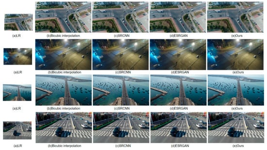
Figure 6. The comparison of overall super-resolution results under a wide field of view.

To verify how our algorithm performs in low-light environments, we filtered images taken at night from the dataset for super-resolution testing. Figure 7 shows the comparison of super-resolution results in dark environments:

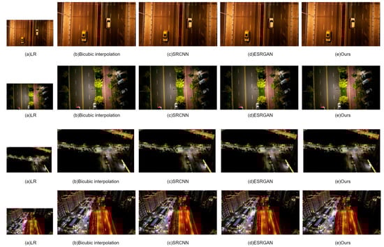
Figure 7. The comparison of super-resolution results in dark environments.

As can be observed from the super-resolution results, the Bicubic Interpolation method yields comparatively poorer super-resolution outcomes. Although both SRCNN and ESRGAN demonstrate competent reconstruction capabilities in well-lit conditions, they exhibit issues with detail blurring in darker, low-light environments. In contrast, our proposed model demonstrates a robust ability to process images captured in dark settings, thereby validating its significant application potential for low-light and nighttime scenarios.

4.3.2. Qualitative Analysis of Super-Resolution Detail Effects

Remote sensing images often contain complex scenes with small targets such as vehicles, pedestrians, and road signs, posing significant challenges for super-resolution algorithms in reconstructing details and textures. To verify our model’s effectiveness in image detail reconstruction, we selected narrow field-of-view images from the dataset for super-resolution testing.

Figure 8 shows the comparison of super-resolution results under a narrow field of view:

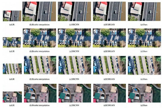
Figure 8. The comparison of super-resolution results under a narrow field of view.

The images display the reconstruction effects of different algorithms on small targets in remote sensing images, clearly showing the differences between them. As a traditional method, Bicubic Interpolation performs poorly in super-resolution reconstruction, with blurred vehicle boundaries, particularly for black vehicles. Furthermore, the boundary between the water body and the ship hull is unclear, and road signs show obvious creasing. In contrast, the two deep learning-based algorithms, SRCNN and ESRGAN, show significant improvement in reconstruction, capable of roughly restoring object boundary information, making vehicles and road signs clearer. However, as shown in Figure 7 (the dark environment comparison figure referenced here from the previous section), in dimly lit scenes, these two algorithms still perform less ideally, where boundary blur and line distortion issues affect the overall image quality. In Figure 8, SRCNN outputs relatively smooth certain details, making edges less prominent. Conversely, ESRGAN over-sharpens some edges, resulting in an unnatural appearance. The algorithm proposed in our paper, RSSRGAN, can better reconstruct detailed edges, finding a more suitable balance between smoothness and sharpness.

To better demonstrate our algorithm’s capability in detail reconstruction, we selected and enlarged detailed portions from the wide field-of-view images for comparison. Figure 9 shows the comparison of detail super-resolution results.

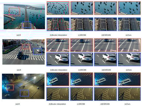
Figure 9. The comparison of detail super-resolution results.

Experimental results indicate that while SRCNN and ESRGAN perform far better than the Bicubic Interpolation algorithm in reconstructing smaller image details, they sometimes still exhibit minor texture blurring. The algorithm proposed in our paper performs excellently in super-resolution reconstruction, not only recovering sharper textures and boundaries but also improving the image’s brightness and color information.

4.4. Quantitative Analysis

GSRGAN denotes Guo’s improved SRGAN model [22], while LSRGAN represents Li’s enhanced SRGAN model [23] (abbreviated as GSRGAN and LSRGAN respectively in the following analysis). Table 1 indicates that the bicubic interpolation method, being a traditional approach, performs poorly across all metrics. SRCNN achieves the best results in PSNR and MSE, demonstrating its powerful capability for pixel-level reconstruction. However, these metrics differ from human visual perception, and its performance in PI and SSIM is moderate. ESRGAN, on the other hand, delivers superior results in PI and SSIM, but its performance in PSNR and MSE is average. Compared to the conventional ESRGAN, both GSRGAN and LSRGAN achieve higher PSNR and SSIM values. Among them, GSRGAN slightly outperforms ESRGAN in PI, though the overall improvement is limited. In contrast, the proposed algorithm RSSRGAN attains higher SSIM and lower PI values on test samples, while also achieving higher PSNR and lower MSE values compared to ESRGAN, GSRGAN, and LSRGAN. Furthermore, although RSSRGAN’s PSNR is lower than that of SRCNN, it significantly surpasses SRCNN in other metrics, particularly PI. This demonstrates that our model not only maintains superior perceptual image quality compared to traditional ESRGAN but also substantially improves pixel-level metrics. Unlike traditional SRCNN, which prioritizes high PSNR, our approach achieves a significant boost in SSIM, PI, and other metrics with only a minor sacrifice in PSNR. Visually, the reconstructed images exhibit closer resemblance to the original images in terms of structure, brightness, and contrast, further confirming their enhanced perceptual quality and overall performance superiority.

Table 1. Super-Resolution Results of Various Methods.

	PSNR	SSIM	MSE	PI
Bicubic Interpolation	21.78	0.737	28.890	7.51
ESRGAN	23.09	0.826	24.975	4.98
SRCNN	29.50	0.774	21.678	7.19
GSRGAN	26.53	0.853	24.641	4.89
LSRGAN	25.48	0.831	24.710	5.23
RSSRGAN	28.77	0.889	23.878	4.33

To compare the computational efficiency and overall performance of these models, we benchmarked the number of parameters, FLOPs, and inference speed of the models mentioned in Table 1. In this experiment, the output is a 1024 × 512 resolution image, performing 4× image super-resolution. The results are shown in Table 2.

Table 2. Comparison of Computational Efficiency and Overall Performance Across Several Models.

	Parameters	FLOPs	Inference Speed (FPS)
Bicubic Interpolation	—	—	>1000
ESRGAN	16.7 M	250 G	15.7
SRCNN	8.1 K	2 G	19.8
GSRGAN	18 M	280 G	14.6
LSRGAN	17 M	260 G	15.2
RSSRGAN	10 M	150 G	20.6

As can be seen from the table, Bicubic Interpolation is not a deep learning model, so its number of parameters and FLOPs are not considered. Although this model achieves extremely fast inference speed, Table 1 shows that the quality of the images it generates is very low. In contrast, SRCNN, with its simple architecture, has a small number of parameters and low FLOPs, and demonstrates fast inference speed. Compared to other traditional models, it processes images more quickly. However, due to its low hardware utilization and inefficient convolution kernel implementation, its actual inference speed is even lower than that of RSSRGAN. The proposed RSSRGAN in this paper, compared to other GAN models, generates higher-quality images with fewer parameters, lower FLOPs, and faster inference speed. Even when compared to the extremely minimalistic architecture of SRCNN, RSSRGAN achieves faster inference speed, demonstrating its performance advantage under similar computational resource consumption and its outstanding role in the field of remote sensing.

4.5. Ablation Study

The experiment used the same training set, test set, data preprocessing pipeline, and hyperparameter settings to ensure the fairness and comparability of the results. The divided test set contained 1000 remote sensing images. The evaluation metrics were Peak Signal-to-Noise Ratio (PSNR), Mean Squared Error (MSE), Structural Similarity Index (SSIM), and Perceptual Index (PI). The relevant metric values after super-resolution reconstruction for each image were calculated, and the average was taken as the final evaluation result.

The results in Table 3 show an improvement of approximately 18.8% in PSNR, 8.0% in SSIM, 3.6% in MSE, and 13.6% in PI. Although the dual-discriminator structure causes a slight decrease in objective metrics such as PSNR and SSIM, it significantly improves subjective metrics like PI, demonstrating its exceptional effectiveness. Additionally, in the experimental setup, we also observed the stability of the training metrics. Here, taking the metric PSNR and the UAVDT dataset as an example, M = 0 indicates not adding the module, and M = 1 indicates adding the module. Figure 10a shows the results when M = 0, where the PSNR mean eventually stabilizes at about 25.6 dB, indicating limitations in extracting multi-scale features when the module is not added. Figure 10b shows the results when M = 1, where the PSNR mean finally reaches about 29.5 dB, significantly enhancing model performance. The results indicate that after adding the module, the model’s ability to extract multi-scale features is greatly enhanced, improving the super-resolution reconstruction effect.

Table 3. Ablation Study Results.

Baseline	Dual Discriminators	Improved Content Loss	Improved Perceptual Loss	PSNR	SSIM	MSE	PI
✔				24.21	0.823	24.775	5.01
✔	✔			24.25	0.821	24.768	4.35
✔		✔		25.94	0.845	24.394	5.02
✔			✔	27.21	0.851	24.151	4.96
✔	✔	✔		26.01	0.846	24.389	4.36
✔	✔		✔	27.19	0.853	24.158	4.32
✔		✔	✔	28.64	0.886	23.865	4.97
✔	✔	✔	✔	28.77	0.889	23.878	4.33

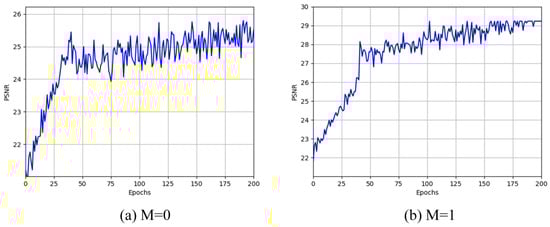
Figure 10. The change in PSNR metrics over 200 training iterations before and after adding the module.

Figure 10 shows the change in PSNR metrics over 200 training iterations before and after adding the module:

To verify our model’s stability, we used the stability of metrics to reflect the model’s stability. For more intuitive demonstration, we introduced discriminator loss and generator loss (The following will be referred to as Dloss and Gloss), two metrics commonly used in GAN experiments, as shown in Figure 11. In Figure 11a, the light blue line represents Dloss without the module, and the dark blue line represents Dloss after adding the module. In Figure 11b, the light blue line represents Gloss without the module, and the dark blue line represents Gloss after adding the module. It can be seen that after adding the module, stability is greatly improved. After stabilization, the standard deviation of Dloss for RSSRGAN is only 76% of the baseline, and the standard deviation of Gloss is only 84% of the baseline.

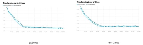
Figure 11. The changing trend of Dloss and Gloss.

Furthermore, we also validated the improvement in training speed. We recorded the training speed for the first 100 iterations, with results shown in Figure 12 (unit: it/s). It can be observed that RSSRGAN’s training speed is significantly higher than the baseline, with an improvement of approximately 9.89%.

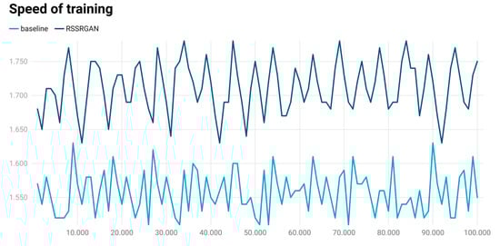
Figure 12. Comparison of training speed (iterations per second) between different models.

5. Discussion

To verify the algorithm’s generalization performance across different scenarios, we conducted experiments using remote sensing data from the Xuanwu Lake area. The dataset was acquired using large aircraft low-altitude remote sensing technology, with flight altitude precisely controlled at about 2500 m, ensuring accurate and reliable data, and a spatial resolution of 0.6 m. This experiment selected two images with a resolution of 10,058 × 7929 pixels. These remote sensing images capture various terrain types, including buildings, lakes, wasteland, and vegetation, effectively representing the characteristics of urban forests. The experimental results are shown in Figure 13. The model can effectively perform super-resolution reconstruction of images such as vehicles, trees, and buildings within the city, effectively capturing details in low-quality images and reconstructing them.

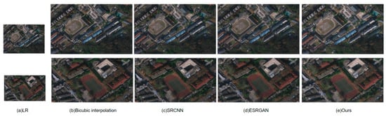
Figure 13. Super-Resolution Results of Xuanwu Lake Remote Sensing Images.

Experimental results show that the proposed model also performs excellently on other remote sensing data, significantly improving image clarity, making blurred boundaries and details sharp, and enhancing information density. Furthermore, the model improves brightness and color information, making originally dim or monochromatic images brighter and more realistic, enhancing the visual experience, and providing a more accurate data foundation for subsequent image analysis. This model can be applied to pixel-level semantic segmentation (using models like U-Net [29], DeepLab [30]), enabling more accurate classification of urban/farmland/forest/water body categories and reducing the impact of mixed pixels. For example, it can better distinguish between sparse and dense buildings, or different crop types. Additionally, it holds great potential for object detection models (e.g., YOLO [31], Faster R-CNN [32]). The model can significantly improve the detection and recognition rates of small man-made targets such as vehicles, ships, and aircraft. In low-resolution images, these targets may consist of only a few pixels, making them difficult to identify. Our model can clarify them, making detection possible.

In summary, the super-resolution model proposed in this research is not merely an independent image processing tool but also a powerful preprocessing technology that can be seamlessly integrated into existing remote sensing processing workflows. By enhancing the quality of raw data from the source, it empowers subsequent various advanced visual tasks, ultimately improving the accuracy and reliability of the entire remote sensing information extraction system, boasting broad prospects for engineering application and commercialization.

6. Conclusions

This study discusses the importance of high-resolution remote sensing images. It proposes RSSRGAN, a Residual Separable Generative Adversarial Network model for remote sensing image super-resolution, which does not rely on hardware improvements and aims to enhance image resolution while strengthening object edges and colors. Specifically, an improved SRGAN model was designed by removing BN layers, using a Sparse Residual Dense Network and Depthwise Separable Convolutional layers to improve computational efficiency, and employing two PatchGAN discriminators to enhance model training stability and convergence. Additionally, Charbonnier loss was incorporated to optimize the content loss function. Experimental results show that the model implemented based on the proposed loss function performs excellently on metrics such as PSNR, SSIM, MSE, and PI, effectively improving the resolution and visual quality of remote sensing images, demonstrating broad application prospects.

Although this study has achieved significant results, several limitations remain. First, the model’s performance still has room for improvement when processing remote sensing images with extreme degradation (e.g., severe motion blur or strong atmospheric interference). Second, the current model is a general-purpose design; future work could explore specialized super-resolution models tailored to specific features (e.g., water bodies, vegetation, urban buildings) to further enhance performance on targeted tasks.

As shown in Figure 14, which uses extremely low-resolution images and images with extremely poor lighting to simulate extreme degradation scenarios. From the super-resolution results, it can be observed that the effectiveness is suboptimal.

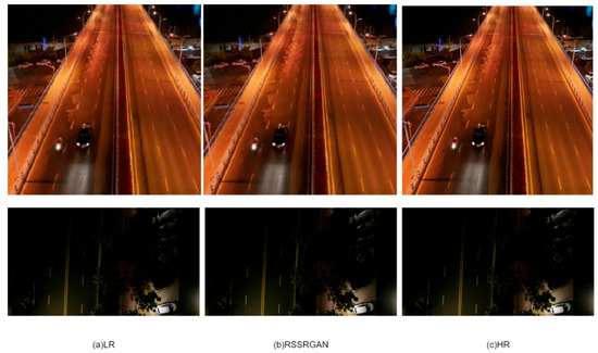
Figure 14. Super-resolution results under extreme degradation environments.

To address the first issue, preprocessing with restoration models such as MPRNet [33] can be applied before using RSSRGAN for subsequent processing. For the second issue, the dataset can be replaced with a target-specific dataset and parameters fine-tuned to improve the model’s adaptability to specific objectives.

In the future, our work will focus on the following directions: (1) Data Expansion and Fusion: Plans to introduce larger-scale, more diverse remote sensing datasets for training, and explore the fusion of multi-source remote sensing data such as radar and multispectral data to extract richer feature information. (2) Algorithm Lightweighting: Commitment to the lightweight design of the model, e.g., through techniques like knowledge distillation and model pruning, to reduce computational complexity and promote its deployment and application on edge computing devices like satellites and airborne platforms. (3) Exploring Emerging Architectures: Continuing to pay attention to and explore the application potential of emerging architectures such as Transformers and Diffusion Models [34] in remote sensing image super-resolution tasks.

References

- Lillesand, T.; Kiefer, R.W.; Chipman, J. Remote Sensing and Image Interpretation; John Wiley & Sons: Hoboken, NJ, USA, 1979. [Google Scholar] [CrossRef]
- Dong, C.; Loy, C.C.; He, K.; Tang, X. Learning a deep convolutional network for image super-resolution. In Proceedings of the European Conference on Computer Vision, Zurich, Switzerland, 6–12 September 2014; Springer International Publishing: Cham, Switzerland, 2014; pp. 184–199. [Google Scholar]
- Goodfellow, I.J.; Pouget-Abadie, J.; Mirza, M.; Xu, B.; Warde-Farley, D.; Ozair, S.; Courville, A.; Bengio, Y. Generative adversarial nets. Adv. Neural Inf. Process. Syst. 2014, 27, 1–9. [Google Scholar]
- Ledig, C.; Theis, L.; Huszar, F.; Caballero, J.; Cunningham, A.; Acosta, A.; Aitken, A.; Tejani, A.; Totz, J.; Wang, Z.; et al. Photo-realistic single image super-resolution using a generative adversarial network. In Proceedings of the IEEE Conference on Computer Vision and Pattern Recognition, Honolulu, HI, USA, 21–26 July 2017; pp. 4681–4690. [Google Scholar]
- Wang, X.; Yu, K.; Wu, S.; Gu, J.; Liu, Y.; Dong, C.; Loy, C.C.; Qiao, Y.; Tang, X. Esrgan: Enhanced super-resolution generative adversarial networks. In Proceedings of the European Conference on Computer Vision (ECCV) Workshops, Munich, Germany, 8–14 September 2018; pp. 63–79. [Google Scholar]
- Mirza, M.; Osindero, S. Conditional Generative Adversarial Nets. Comput. Sci. 2014, 2672–2680. [Google Scholar] [CrossRef]
- Radford, A.; Metz, L.; Chintala, S. Unsupervised representation learning with deep convolutional generative adversarial networks. arXiv 2015, arXiv:1511.06434. [Google Scholar]
- Zhu, J.-Y.; Park, T.; Isola, P.; Alexei, A.E. Unpaired image-to-image translation using cycle-consistent adversarial networks. In Proceedings of the IEEE International Conference on Computer Vision, Venice, Italy, 22–29 October 2017; pp. 2223–2232. [Google Scholar]
- Keys, R. Cubic convolution interpolation for digital image processing. IEEE Trans. Acoust. Speech Signal Process. 1981, 29, 1153–1160. [Google Scholar] [CrossRef]
- Yang, J.; Wright, J.; Huang, T.; Ma, Y. Image super-resolution as sparse representation of raw image patches. In Proceedings of the IEEE Conference on Computer Vision and Pattern Recognition, Anchorage, AK, USA, 23–28 June 2008; pp. 1–8. [Google Scholar]
- Hinton, G.E.; Salakhutdinov, R.R. Reducing the dimensionality of data with neural networks. Science 2006, 313, 504–507. [Google Scholar] [CrossRef] [PubMed]
- He, K.; Zhang, X.; Ren, S.; Sun, J. Deep residual learning for image recognition. In Proceedings of the IEEE Conference on Computer Vision and Pattern Recognition, Las Vegas, NV, USA, 27–30 June 2016; pp. 770–778. [Google Scholar]
- Kim, J.; Lee, J.K.; Lee, K.M. Accurate image super-resolution using very deep convolutional networks. In Proceedings of the IEEE Conference on Computer Vision and Pattern Recognition, Las Vegas, NV, USA, 27–30 June 2016; pp. 1646–1654. [Google Scholar]
- Shi, W.; Caballero, J.; Huszár, F.; Totz, J.; Aitken, A.P.; Bishop, R.; Rueckert, D.; Wang, Z. Real-time single image and video super-resolution using an efficient sub-pixel convolutional neural network. In Proceedings of the IEEE Conference on Computer Vision and Pattern Recognition, Las Vegas, NV, USA, 27–30 June 2016; pp. 1874–1883. [Google Scholar]
- Lim, B.; Son, S.; Kim, H.; Nah, S.; Lee, K.M. Enhanced deep residual networks for single image super-resolution. In Proceedings of the IEEE Conference on Computer Vision and Pattern Recognition Workshops, Honolulu, HI, USA, 21–26 July 2017; pp. 136–144. [Google Scholar]
- Zhang, Y.; Li, K.; Li, K.; Wang, L.; Zhong, B.; Fu, Y. Image super-resolution using very deep residual channel attention networks. In Proceedings of the European Conference on Computer Vision (ECCV), Munich, Germany, 8–14 September 2018; pp. 286–301. [Google Scholar]
- Zhang, Y.; Li, K.; Li, K.; Zhong, B.; Fu, Y. Residual non-local attention networks for image restoration. arXiv 2019, arXiv:1903.10082. [Google Scholar] [CrossRef]
- Dosovitskiy, A.; Beyer, L.; Kolesnikov, A.; Weissenborn, D.; Zhai, X.; Unterthiner, T.; Dehghani, M.; Minderer, M.; Heigold, G.; Gelly, S.; et al. An image is worth 16 × 16 words: Transformers for image recognition at scale. arXiv 2020, arXiv:2010.11929. [Google Scholar]
- Liang, J.; Cao, J.; Sun, G.; Zhang, K.; Van Gool, L.; Timofte, R. Swinir: Image restoration using swin transformer. In Proceedings of the IEEE/CVF International Conference on Computer Vision, Virtual, 11–17 October 2021; pp. 1833–1844. [Google Scholar]
- Wang, X.; Xie, L.; Dong, C.; Shan, Y. Real-esrgan: Training real-world blind super-resolution with pure synthetic data. In Proceedings of the IEEE/CVF International Conference on Computer Vision, Virtual, 11–17 October 2021; pp. 1905–1914. [Google Scholar]
- Zhou, Q. Superresolution reconstruction of remote sensing image based on generative adversarial network. Wirel. Commun. Mob. Comput. 2022, 2022, 9114911. [Google Scholar] [CrossRef]
- Guo, J.; Lv, F.; Shen, J.; Liu, J.; Wang, M. An improved generative adversarial network for remote sensing image super-resolution. IET Image Process. 2023, 17, 1852–1863. [Google Scholar] [CrossRef]
- Li, R.; Liu, W.; Gong, W.; Zhu, X.; Wang, X. Super resolution for single satellite image using a generative adversarial network. ISPRS Ann. Photogramm. Remote Sens. Spat. Inf. Sci. 2022, V-3-2022, 591–596. [Google Scholar] [CrossRef]
- Xu, B.; Wang, N.; Chen, T.; Li, M. Empirical evaluation of rectified activations in convolutional network. arXiv 2015, arXiv:1505.00853. [Google Scholar] [CrossRef]
- Horn, B.K.P.; Schunck, B.G. Determining optical flow. Artif. Intell. 1981, 17, 185–203. [Google Scholar] [CrossRef]
- Rudin, L.I.; Osher, S.; Fatemi, E. Nonlinear total variation based noise removal algorithms. Phys. D Nonlinear Phenom. 1992, 60, 259–268. [Google Scholar] [CrossRef]
- Wang, Z. Image quality assessment: Form error visibility to structural similarity. IEEE Trans. Image Process. 2004, 13, 604–606. [Google Scholar]
- Mittal, A.; Soundararajan, R.; Bovik, A.C. Making a “completely blind” image quality analyzer. IEEE Signal Process. Lett. 2012, 20, 209–212. [Google Scholar] [CrossRef]
- Ronneberger, O.; Fischer, P.; Brox, T. U-net: Convolutional networks for biomedical image segmentation. In Proceedings of the International Conference on Medical Image Computing and Computer-Assisted Intervention, Munich, Germany, 5–9 October 2015; Springer International Publishing: Cham, Switzerland, 2015; pp. 234–241. [Google Scholar]
- Chen, L.-C.; Zhu, Y.; Papandreou, G.; Schroff, F.; Adam, H. Encoder-decoder with atrous separable convolution for semantic image segmentation. In Proceedings of the European Conference on Computer Vision (ECCV), Munich, Germany, 8–14 September 2018; pp. 801–818. [Google Scholar]
- Redmon, J.; Divvala, S.; Girshick, R.; Farhadi, A. You only look once: Unified, real-time object detection. In Proceedings of the IEEE Conference on Computer Vision and Pattern Recognition, Las Vegas, NV, USA, 27–30 June 2016; pp. 779–788. [Google Scholar]
- Ren, S.; He, K.; Girshick, R.; Sun, J. Faster R-CNN: Towards real-time object detection with region proposal networks. IEEE Trans. Pattern Anal. Mach. Intell. 2016, 39, 1137–1149. [Google Scholar] [CrossRef] [PubMed]
- Zamir, S.W.; Arora, A.; Khan, S.; Hayat, M.; Khan, F.S.; Yang, M.-H.; Shao, L. Multi-stage progressive image restoration. In Proceedings of the IEEE/CVF Conference on Computer Vision and Pattern Recognition, Virtual, 19–25 June 2021; pp. 14821–14831. [Google Scholar]
- Sohl-Dickstein, J.; Weiss, E.A.; Maheswaranathan, N.; Ganguli, S. Deep unsupervised learning using nonequilibrium thermodynamics. In Proceedings of the International Conference on Machine Learning, PMLR, Lille, France, 6–11 July 2015; pp. 2256–2265. [Google Scholar]
Disclaimer/Publisher’s Note: The statements, opinions and data contained in all publications are solely those of the individual author(s) and contributor(s) and not of MDPI and/or the editor(s). MDPI and/or the editor(s) disclaim responsibility for any injury to people or property resulting from any ideas, methods, instructions or products referred to in the content. |
© 2025 by the authors. Licensee MDPI, Basel, Switzerland. This article is an open access article distributed under the terms and conditions of the Creative Commons Attribution (CC BY) license.