Highlights
What are the main findings?
- A SHAP–correlation feature selection strategy (aggregated mean absolute SHAP values with Pearson analysis) enhanced robustness and identified critical predictive variables.
- Multi-source feature fusion significantly improved LAI retrieval accuracy across models, and LAI showed a distinct coastal-to-inland spatial gradient.
What are the implications of the main findings?
- Fusing hyperspectral and LiDAR with SHAP–correlation selection provides a robust, generalizable pathway for high-precision LAI mapping in heterogeneous wetlands.
- The mapped coastal–inland LAI gradient offers a quantitative basis for ecological assessment, supporting vegetation succession monitoring, and water–salt regulation practices in the Yellow River Delta.
Abstract
The leaf area index (LAI) serves as a critical parameter for assessing wetland ecosystem functions, and accurate LAI retrieval holds substantial significance for wetland conservation and ecological monitoring. To address the spatial constraints of traditional ground-based measurements and the limited accuracy of single-source remote sensing data, this study utilized unmanned aerial vehicle (UAV)-borne hyperspectral and LiDAR sensors to acquire high-quality multi-source remote sensing data of coastal wetlands in the Yellow River Delta. Three machine learning algorithms—random forest (RF), Extreme Gradient Boosting (XGBoost), and Categorical Boosting (CatBoost)—were employed for LAI retrieval modeling. A total of 38 vegetation indices (VIs) and 12-point cloud features (PCFs) were extracted from hyperspectral imagery and LiDAR point cloud data, respectively. Pearson correlation analysis and the Shapley Additive Explanations (SHAP) method were integrated to identify and select the most informative VIs and PCFs. The performance of LAI retrieval models built on single-source features (VIs or PCFs) or multi-source feature fusion was evaluated using the coefficient of determination (R2) and root mean square error (RMSE). The main findings are as follows: (1) Multi-source feature fusion significantly improved LAI retrieval accuracy, with the RF model achieving the highest performance (R2 = 0.968, RMSE = 0.125). (2) LiDAR-derived structural metrics and hyperspectral-derived vegetation indices were identified as critical factors for accurate LAI retrieval. (3) The feature selection method integrating mean absolute SHAP values (|SHAP| values) with Pearson correlation analysis enhanced model robustness. (4) The intertidal zone exhibited pronounced spatial heterogeneity in the vegetation LAI distribution.
1. Introduction
Wetlands represent ecologically vital ecosystems on a global scale, playing unique and irreplaceable roles in sustaining biodiversity, regulating climate, and purifying water quality [1]. The leaf area index (LAI), as a key parameter for assessing the growth status of wetland vegetation and the functioning of wetland ecosystems, is critical for evaluating vegetation health [2,3]. Consequently, the accurate acquisition of wetland LAI provides a crucial scientific foundation for the conservation, management, and ecological restoration of these ecologically valuable wetland ecosystems.
Traditional methods for measuring the LAI of wetland vegetation primarily include direct destructive measurements and ground-based optical instrumentations. The direct destructive measurement method calculates the LAI by harvesting plant leaves and quantifying their total area. Although this approach delivers high accuracy, it is inherently labor-intensive, time-consuming, and destructive to vegetation; these limitations render it unsuitable for the dynamic monitoring of large-scale wetlands [4]. Ground-based optical instruments, by contrast, suffer from constrained measurement ranges; for example, the LAI-2200 plant canopy analyzer only captures point-scale data, and its accuracy is heavily influenced by topography and vegetation distribution patterns [5]. This inadequacy prevents it from comprehensively characterizing the spatial heterogeneity of wetland vegetation.
Satellite remote sensing technologies offer advantages such as large-scale coverage and high temporal frequency, but still face notable limitations in LAI retrieval, including low spatial resolution and restricted spectral information. These constraints hinder their ability to fully meet the requirements of high-precision vegetation LAI retrieval [6,7,8]. To address the limitations of traditional measurement methods and satellite remote sensing in capturing spatial and spectral information, unmanned aerial vehicle (UAV)-based remote sensing provides a novel pathway for refined LAI retrieval. High-resolution multi-source remote sensing data can be obtained by mounting diverse sensor types on UAVs. Among these sensors, multispectral and hyperspectral systems capture high-resolution vegetation spectral information, facilitating detailed characterization of canopy spectral trails [9]. In contrast, Light Detection and Ranging (LiDAR) systems generate point clouds that penetrate vegetation canopies to capture vertical structural information, offering critical three-dimensional structural insights for LAI estimation [10,11]. Meanwhile, machine learning algorithms, owing to their robust adaptability to high-dimensional, multi-source, and nonlinear datasets, have emerged as essential tools for retrieving LAI and other vegetation biophysical parameters from remote sensing data [12].
In recent years, the integration of UAV-borne multi-source remote sensing and machine learning has offered diverse technical solutions for LAI retrieval. Machine learning optimization strategies based on spectral response mechanisms improve the representation of spectral features through first- and second-order derivative transformations and the screening of sensitive vegetation indices [13]. Integrated with intelligent parameter optimization, these methods have been successfully applied to LAI retrieval modeling for crops and wetland vegetation [14], thereby effectively validating the feasibility of integrating UAV hyperspectral data with machine learning for high-precision LAI estimation. Liang et al. [15,16] utilized the PROSAIL model to generate simulated datasets, analyzed various hyperspectral vegetation indices (VIs), and constructed hybrid inversion models by combining artificial neural networks (ANNs), random forest regression (RFR), and other algorithms. They found that the optimized soil-adjusted vegetation index (OSAVI) and the modified triangular vegetation index (MTVI2) exhibited the highest sensitivity to the LAI, and that RFR delivered superior estimation when prior knowledge was incorporated. LiDAR point cloud data can be used to represent three-dimensional (3D) canopy structures with high spatial accuracy; thus, they enable the construction of physically interpretable LAI estimation models and thus exhibit remarkable advantages in LAI retrieval [17]. For example, Wang and Fang [10] derived gap fraction and contact frequency from LiDAR data and achieved high LAI estimation accuracy through the combination of regression and physical modeling approaches. Similarly, Yang et al. [17] validated the significant advantages of LiDAR-derived structural features in structural accuracy and spatial adaptability through a slope-aware filtering algorithm, revealing strong correlations with an in situ measured effective LAI.
However, the saturation effects of spectral features and the lack of biochemical sensitivity in LiDAR point clouds still constrain the accuracy and generalization ability of LAI retrieval models [2,10]. Current research has thus focused on the synergistic utilization of multi-source remote sensing features, with the goal of integrating the biochemical sensitivity of spectral data with the 3D structural characterization ability of LiDAR [18,19,20]. This approach enables the technical limitations of single-source data to be overcome, realizes a comprehensive characterization of dual-dimension “spectral + structural” features, and improves the accuracy and stability of LAI retrieval. In particular, related studies remain relatively scarce in the complex ecological contexts of wetlands, thereby underscoring considerable potential for future research and applications.
This study focused on coastal wetland vegetation in the Yellow River Delta, and hyperspectral imagery and LiDAR point cloud data were specifically acquired for the coastal–inland transition zone. Through the optimization and screening of multi-source remote sensing feature variables, machine learning algorithms were employed to construct LAI retrieval models for wetland vegetation. The objectives were to investigate the role of hyperspectral–LiDAR feature fusion in enhancing LAI estimation accuracy, identify the optimal LAI retrieval approach, and generate maps of the wetland vegetation LAI.
2. Materials and Methods
2.1. Study Area
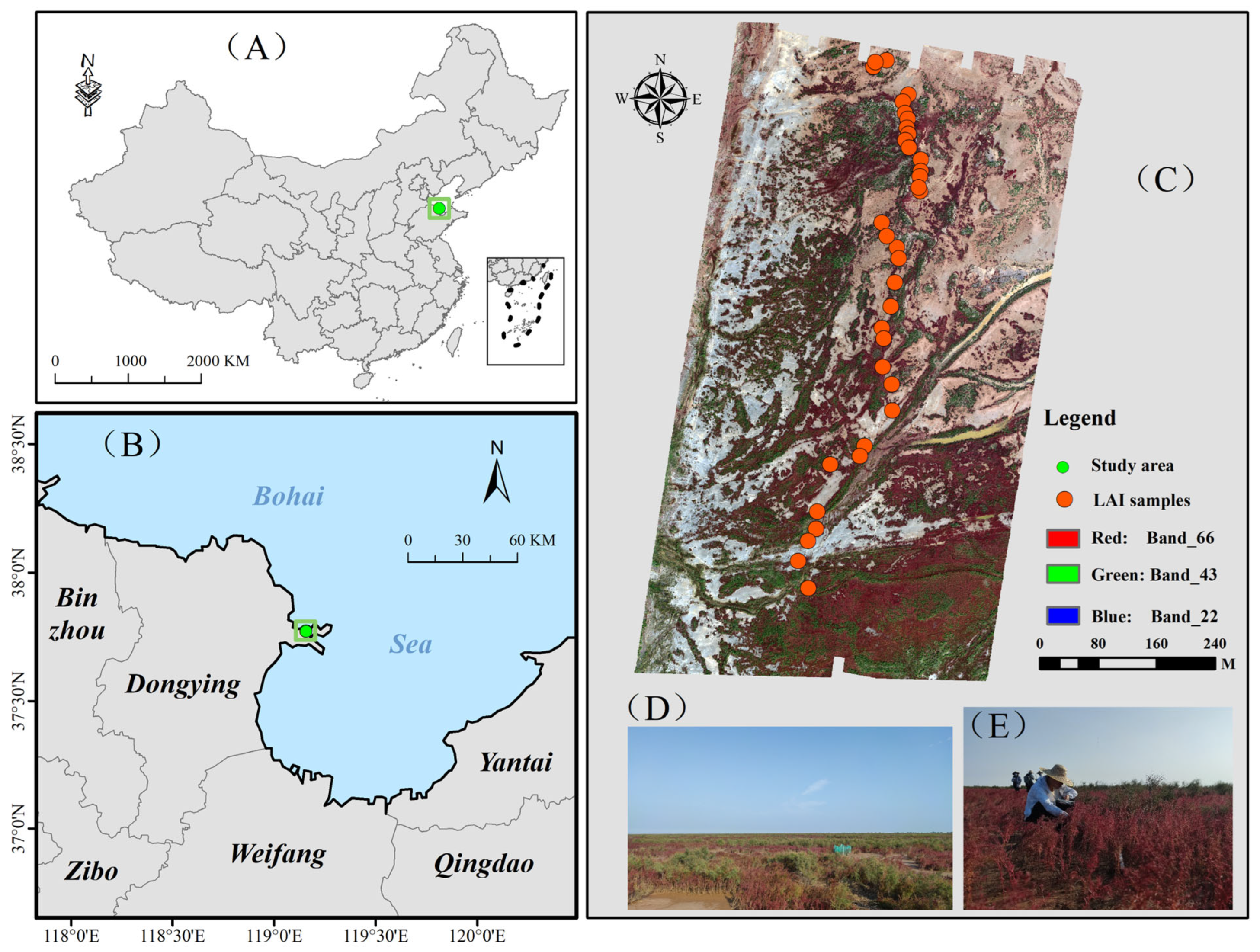
The study area is located in the intertidal wetland of the Yellow River Delta (37°24′–38°10′N, 118°15′–119°19′E) (Figure 1), spanning from the coastal zone to inland. This region is characterized by significant tidal influences on coastal processes, with a mean annual temperature ranging from 12 to 13 °C and an average annual precipitation of approximately 550 to 600 mm yr−1. The region falls within the warm temperate semi-humid monsoon climate zone, exhibits marked seasonal hydrological variability, and has predominantly saline–alkaline soils.
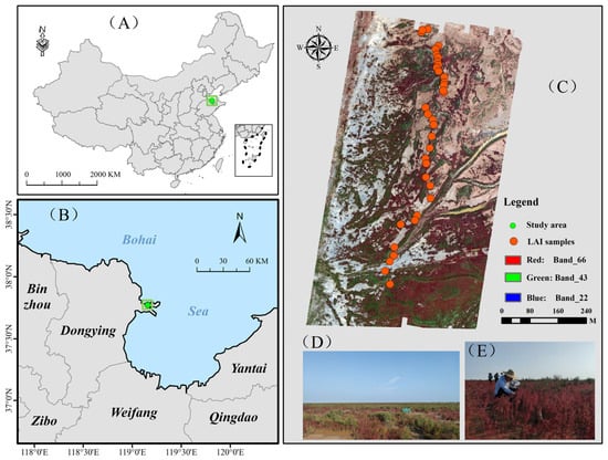
Figure 1.
Location of the study area in the Yellow River Delta wetlands. The green dots in (A) and (B) denote the location of the study area within the geographical boundaries of China and Dongying city, respectively. The orange-yellow dots in (C) represent the sampling points for in situ LAI measurements, whereas the background imagery of (C) is an RGB composite image derived from UAV-borne hyperspectral datasets. (D,E) illustrate representative on-site visual documentation of the study area, capturing the actual vegetation of the research site.
The Yellow River Delta contains diverse wetland types, i.e., permanent freshwater wetlands, seasonal wetlands, intertidal mudflats, and artificial wetlands. The vegetation in this delta is highly sensitive to hydrological fluctuations and human disturbances. For this study, the coastal–inland transitional vegetation belt of the Yellow River Delta was selected as the core study area for LAI retrieval. The dominant vegetation consists of typical halophytic and salt-tolerant species such as Tamarix chinensis, Phragmites australis, and Suaeda salsa [21].
2.2. Data Acquisition and Preprocessing
2.2.1. UAV-Borne Hyperspectral Imagery
UAV-borne hyperspectral imagery was acquired between 25 and 27 September 2024, within 10:00–14:00 local time, under clear sky and light wind conditions to ensure stable illumination for spectral measurements. These flights were organized within the same acquisition campaign as the LiDAR survey so as to maintain the temporal consistency of the multi-source datasets. Specifically, hyperspectral data were collected using an M300 RTK UAV (DJI, Shenzhen, China) integrated with a PIKA L hyperspectral imaging sensor (Resonon, Bozeman, MT, USA) (Figure 2a,b, Table 1). The raw hyperspectral imagery were preprocessed using MEGA CUBE V2.15.1 software in three core steps: geometric correction, radiometric calibration, and reflectance conversion. These steps eliminated spatial distortions, removed data stitching, and derived surface reflectance. After preprocessing, ArcMap 10.2 (Esri, Redlands, CA, USA) and ENVI 5.1 (L3Harris Geospatial, Boulder, CO, USA) were utilized to perform georeferencing (aligning imagery with the WGS84 coordinate system), strip mosaicking, and data format conversion. This comprehensive processing workflow generated orthorectified hyperspectral reflectance datasets with consistent spatial and spectral integrity.
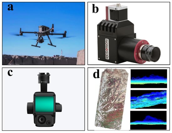
Figure 2.
UAV-borne hyperspectral and LiDAR data acquisition system: (a) DJI M300 RTK UAV platform; (b) PIKA L hyperspectral imaging sensor; (c) DJI L1 LiDAR sensor; (d) hyperspectral and LiDAR data from the study area.

Table 1.
Parameters of the UAV-borne hyperspectral and LiDAR systems.
2.2.2. UAV-Borne LiDAR Data
The point cloud data of the study area was collected using an L1 LiDAR sensor (DJI, China) with an M300 RTK UAV platform (Figure 2a,c, Table 1). For each flight block, a LiDAR survey was carried out between 14:00 and 15:00 local time on the same days as the hyperspectral flights. The LiDAR acquisition for a given block was scheduled immediately after the corresponding hyperspectral flight, and the time interval between the two acquisitions was kept within approximately 30 min, so that illumination conditions and canopy status remained comparable at the plot scale. Because LiDAR measurements are much less sensitive to illumination changes than hyperspectral imagery, the LiDAR missions were deliberately scheduled in the later part of the 10:00–15:00 window to prioritize optimal lighting conditions for hyperspectral data. The point cloud dataset included the 3D geospatial coordinates (x, y, z) of each laser return, scan angle, return intensity, and GPS timestamp information. First, the raw point cloud data were processed using DJI Terra 5.1.0 software (DJI, Shenzhen, China) for trajectory calculation and flight strip mosaicking. Subsequently, LiDAR360 5.2 software (GreenValley International, Shanghai, China) was employed for sequential noise removal, filtering, and ground point classification. Finally, a digital elevation model (DEM) was generated using an irregular triangular network (TIN) interpolation method. The point cloud data were then normalized against the DEM to distinguish vegetation canopy points from the underlying terrain, enabling subsequent extraction of vegetation structural features.
2.2.3. In Situ LAI Measurements
The survey period was deliberately scheduled in late September, which corresponds to a relatively stable late growing season when the canopies of the dominant species (Suaeda salsa, Tamarix chinensis, and Phragmites australis) are fully developed but before large-scale senescence. Therefore, current LAI retrieval models are primarily representative of wetland vegetation conditions during this phenological stage. In this study, ground-based in situ measurements of wetland vegetation LAI were conducted from 24 to 27 September 2024, between 09:00 and 16:00 local time. Sampling plots of 0.5 m × 0.5 m were established, and the canopy LAI was measured using an LAI-2200C plant canopy analyzer (Li-Cor Biosciences, Lincoln, NE, USA) at five different distinct azimuth angles (to account for directional heterogeneity in canopy structure). The average of these values was taken as the ground-truth LAI of each plot.
For plots dominated by Suaeda salsa, we selected locations where canopy height was at least 10 cm and positioned the LAI-2200C sensor head horizontally at approximately 5 cm above the ground surface. For these measurements, the sensor head was equipped with a 270° view cap, leaving a 90° viewing sector open to restrict the field of view and minimize interference from adjacent bare soil, nearby water surfaces, and the operator. The open sector was oriented toward the sun, while the operator squatted behind the masked 270° sector and held the sensor head using the extension rod, keeping the body at a distance of about 1 m from the fisheye lens to avoid entering the field of view or casting shadows.
A high-precision A100 RTK device (Qianxun S.I. Inc., Shanghai, China) was used to record the geospatial coordinates (WGS84 coordinate system) of the plot centers, with a positioning accuracy of <2 cm. A total of 110 plots were established and measured across the entire study area. The measured LAI values of wetland vegetation spanned a range from 0.173 to 3.42, with a mean of 1.57 and a coefficient of variation of 42.93% (Table 2). Among the dominant species, Suaeda salsa, Tamarix chinensis, and Phragmites australis exhibited mean LAI values of 1.30, 1.70, and 1.78, respectively, accompanied with standard deviations of 0.68, 0.46, and 0.88.

Table 2.
Statistics of vegetation LAI.
2.3. Feature Extraction and Selection
2.3.1. VI Calculation
A total of 38 VIs, including commonly used difference-based, ratio-based, and nonlinear indices sensitive to the LAI, were selected as variables for LAI retrieval. The detailed calculation formulas for these VIs are provided in Table 3. Given that the hyperspectral dataset contained 150 spectral bands, the hyperspectral bands most closely matching or identical to the corresponding bands specified in the original VI formulas were selected for index calculation. The computation and extraction of VIs for the sampling plots were performed using Python 3.8 to ensure computational reproducibility.

Table 3.
Thirty-eight VIs and their formulas.
2.3.2. LiDAR Point Cloud Feature (PCF) Extraction
LiDAR data preprocessing involved noise removal, ground point classification, and DEM generation using the TIN interpolation method. Twelve PCFs were extracted from the preprocessed point cloud of the study area, including height coefficient of variation (HCV), mean height (Hmean), minimum height (Hmin), canopy cover (Fcover), gap fraction (FG), canopy relief ratio (RCR), and height percentiles (H1th, H10th, H25th, H50th, H75th, H99th). Specifically, HCV represents the degree of vertical heterogeneity of the canopy; Hmean, the average plant height; Hmin, the minimum plant height; Fcover, the percentage of the vertical projection area of the crop canopy on the ground relative to the total area; FG, the ratio of ground points to total points; RCR, a three-dimensional measure of the horizontal and vertical heterogeneity of the vegetation canopy; and H1th, H10th, H25th, H50th, H75th, and H99th, the heights above ground at the 1%, 10%, 25%, 50%, 75%, and 99% height percentiles within each sampling plot. All LiDAR PCF extractions for the sampling plots were implemented in Python to handle point cloud data efficiently. Vegetation structural features such as HCV, Fcover, and FG were calculated at a 0.1 m × 0.1 m grid resolution, and plot-level structural metrics were further aggregated by averaging grid-level features within each 0.5 m × 0.5 m field plot.
2.3.3. SHAP–Correlation Feature Selection Strategy
To enhance the performance of wetland vegetation LAI retrieval models, reduce computational complexity, and improve generalization ability for model robustness, a systematic feature selection framework was adopted to retain key features while removing redundant information for model optimization. The specific procedure was implemented as follows:
- Pearson correlation analysis was conducted to quantify the strengths of linear relationships among all selected features (VIs and PCFs) and evaluate potential collinearity within the initial feature set.
- Three machine learning models (RF, XGBoost, and CatBoost) were then utilized to calculate the mean absolute SHAP values of all features, which quantified the relative contribution of each feature to model outputs. These features were subsequently selected based on a pre-defined threshold (retaining features with mean SHAP values in the top 50% of all features).
- Finally, for the features retained after importance-based filtering, highly collinear variables (correlation coefficient |r| > 0.95) were identified and removed based on correlation analysis to avoid over-reliance on a single collinearity metric. The resulting optimal feature subset was ultimately used for the construction of wetland vegetation LAI retrieval models.
Because our retrieval models are tree-based ensembles (RF, XGBoost, and CatBoost), the correlation filter was not intended to enforce a strict de-correlation rule (e.g., |r| < 0.8), as is often implemented for parametric linear models. Instead, we applied Pearson filtering after SHAP-based importance screening and used a conservative threshold (|r| > 0.95) mainly to remove near-duplicate predictors (e.g., functionally very similar VIs or highly overlapping height-percentile PCFs). Recent studies indicate that random forests and related tree-ensemble models can maintain stable predictive performance in the presence of correlated predictors, whereas overly aggressive removal of correlated variables may discard useful complementary information [42,43,44]. Therefore, we retained correlated-but-informative features and removed only the almost redundant ones to keep both spectral (VIs) and structural (PCFs) information for LAI retrieval.
2.4. Machine Learning Modeling for LAI Retrieval
2.4.1. Model Selection and Parameter Tuning
All samples were first randomly shuffled and then randomly divided into training and independent testing sets at an 8:2 ratio; model construction and parameter optimization were conducted exclusively on the training set. The filtered VI, PCF, and fused feature subsets were separately input into the RF, XGBoost, and CatBoost models. The models’ LAI retrieval accuracies were then compared to determine the optimal modeling framework. Model predictive performance was assessed on the independent testing set using the coefficient of determination (R2) and root mean square error (RMSE).
In total, 110 LAI sampling points were initially established. When extracting point-based structural metrics from the LiDAR point cloud at these locations, 13 sampling points returned null values for all height-based PCFs, likely due to locally incomplete point cloud coverage or very low point density in low and patchy Suaeda salsa stands. To avoid introducing missing values into the fused feature set, these 13 points were removed, and the remaining 97 points were used for VIs + PCF fusion modeling. Among the discarded points, 10 were dominated by Suaeda salsa and three by Tamarix chinensis. Additionally, a comparison of vegetation-type composition and LAI statistics before and after removing these points (Table 4) shows that the variation coefficient of LAI for dominant species varies within 4 percentage points, suggesting that this exclusion is unlikely to introduce substantial selection bias into the modeling dataset.

Table 4.
Descriptive statistics of LAI for the full sample set (110 plots) and fusion subset (97 plots) by vegetation type.
To construct the random forest (RF) model, the optimal configuration was determined using grid search and 5-fold cross-validation. The parameter ranges tested during the grid search are listed in Table 5. The final parameters were as follows: n_estimators = 1200 (number of decision trees in the forest), max_depth = 16 (maximum depth of individual decision trees), max_features = 0.8 (proportion of features considered for splitting at each node), and min_samples_leaf = 2 (minimum number of samples required at a leaf node).

Table 5.
Hyperparameter tuning for RF, XGBoost, and CatBoost models.
For the XGBoost model, parameter optimization was conducted using a combination of grid search and 5-fold cross-validation to mitigate overfitting by leveraging subset validation. The parameter ranges tested during the grid search are listed in Table 5. The optimal parameters were as follows: learning_rate = 0.03 (step size shrinkage controlling the learning rate of each boosting step), max_depth = 7 (maximum depth of individual decision trees), subsample = 0.6 (proportion of training samples randomly selected for each boosting iteration), and colsample_bytree = 0.9 (proportion of features randomly selected to grow each tree).
For the CatBoost model, a Bayesian sampling strategy combined with 5-fold cross-validation was employed to enhance model stability and prevent overfitting. The parameter ranges tested during the Bayesian optimization process are listed in Table 5. The optimal parameters after Bayesian optimization were as follows: depth = 5 (maximum depth of individual decision trees), learning_rate = 0.05 (step size shrinkage controlling the learning rate of each boosting step), n_estimators = 800 (number of boosting trees), and min_data_in_leaf = 50 (minimum number of samples required at a leaf node).
2.4.2. Performance Evaluation for LAI Retrieval Model
R2 and RMSE were used as evaluation metrics for model performance [45]. R2 indicates the goodness of fit between the model and the data, while RMSE reflects the degree of dispersion of the observed values around the regression line. A higher R2 and a lower RMSE indicate greater estimation accuracy. The performances of all models were accurately compared, and the optimal model in terms of performance was further applied to generate a fine-scale map of the wetland vegetation LAI.
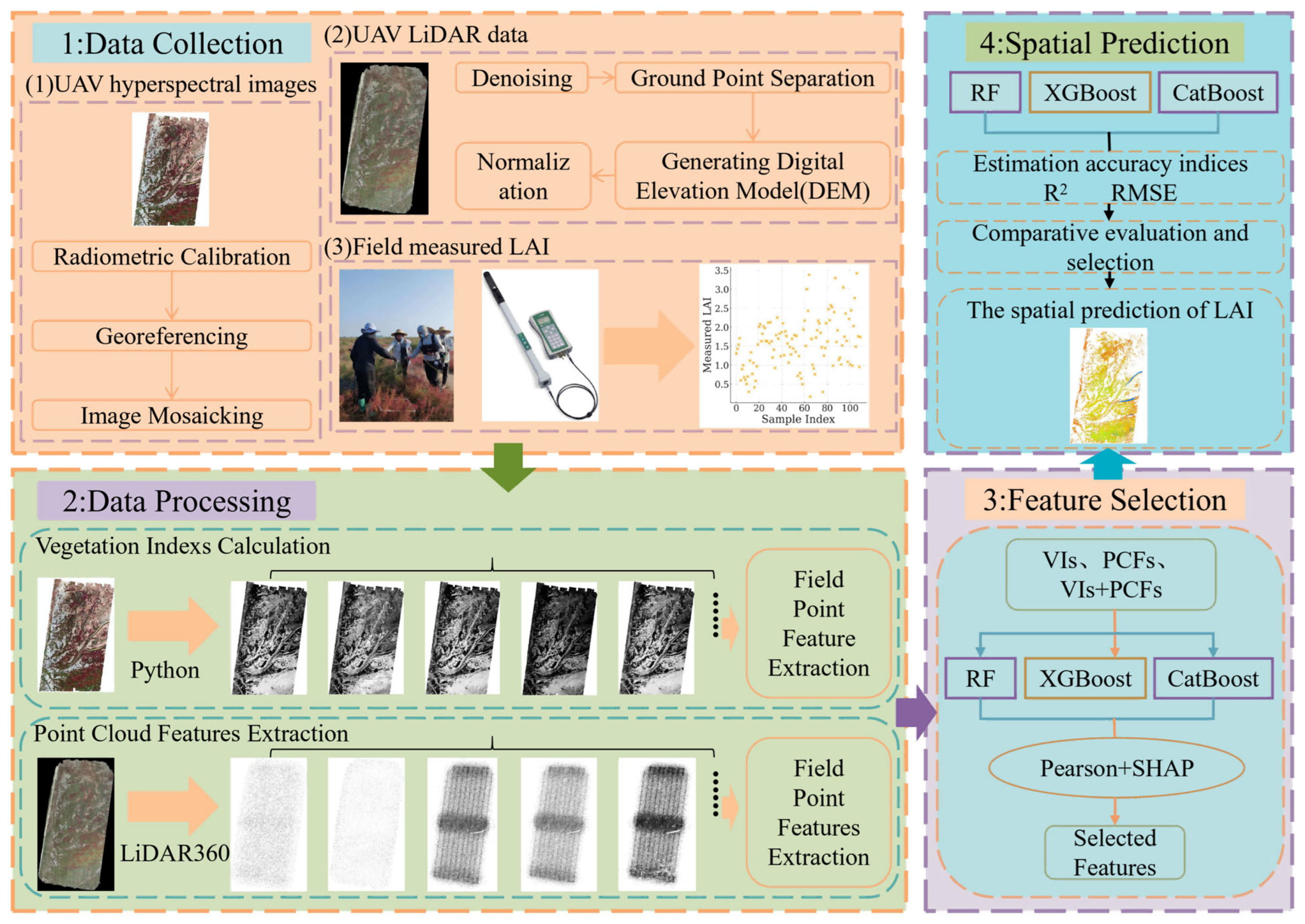
This study systematically compared the LAI retrieval accuracy of hyperspectral vegetation indices (VIs), LiDAR point cloud features (PCFs), and their fused features (VIs + PCFs) across three machine learning models to explore the complementarity roles of multi-source remote sensing features. The methodological workflow is structured into four interconnected phases (Figure 3): (1) synchronous acquisition of in situ LAI ground-truth measurements, UAV-borne hyperspectral imagery, and LiDAR point cloud data; (2) sequential data preprocessing and feature extraction (VI calculation, PCF extraction); (3) SHAP–correlation-integrated feature selection and LAI retrieval modeling using RF, XGBoost, and CatBoost; and (4) quantitative model evaluation and fine-scale LAI spatial mapping. This framework ensures the consistency of multi-source data fusion and modeling, laying the foundation for accurate LAI retrieval.
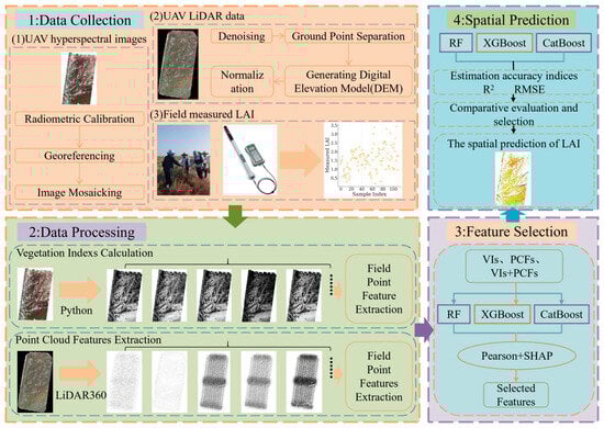
Figure 3.
Technical framework of this study.
3. Results
3.1. Inter- and Intra-Feature Correlation Patterns
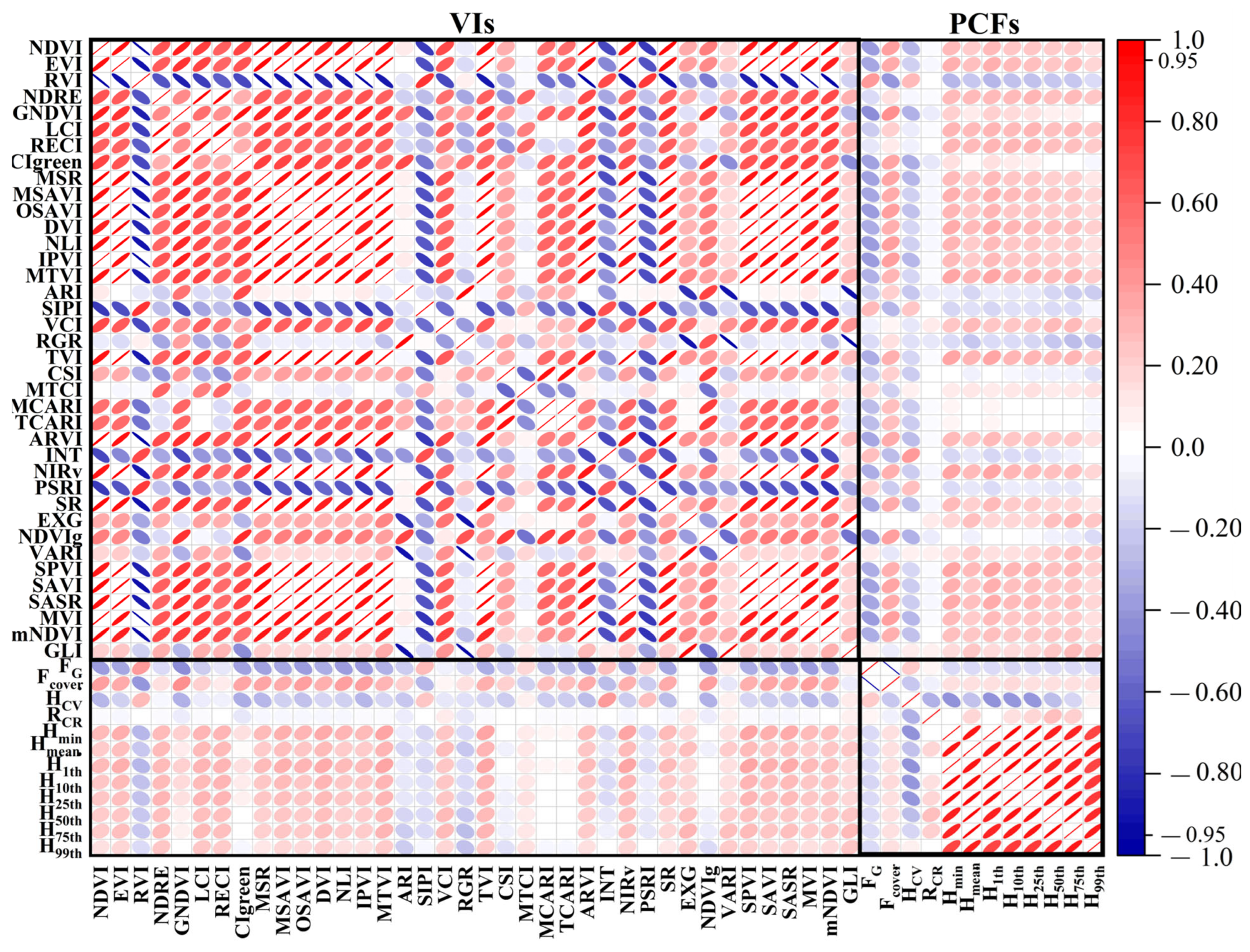
The Pearson correlation coefficients for VIs and PCFs were calculated both inter-feature (between VIs and PCFs) and intra-group (within VIs or within PCFs), with correlation patterns visualized using heatmaps (Figure 4). This analysis explicitly assessed inter-feature redundancy and cross-feature complementarity—two critical prerequisites for multi-source feature fusion.
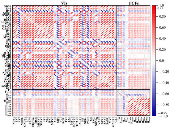
Figure 4.
Correlation heatmap between VIs and PCFs, including inter- and intra-feature correlation analysis.
3.1.1. Inter-Feature Correlation Between VIs and PCFs
VIs and PCFs exhibited weak linear associations overall, with an absolute Pearson correlation coefficient |r| < 0.45. For example, the GNDVI correlated weakly with H25th (r = 0.16), while the ARVI showed a moderate negative correlation with HCV (r = −0.28). This weak inter-feature correlation is consistent with their distinct information capture mechanisms. VIs predominantly encode the spectral and biochemical attributes of vegetation (e.g., chlorophyll content, leaf water content), whereas LiDAR-derived PCFs mainly characterize the 3D canopy structure traits (e.g., height distribution, canopy porosity). Such minimal inter-feature redundancy confirms that VIs and PCFs provide complementary vegetation information for fusing these features to enhance LAI retrieval accuracy.
3.1.2. Intra-Feature Correlation Within VIs and PCFs
Notably, strong intra-feature collinearity was detected among subsets of VIs, with |r| exceeding 0.95 for multiple pairs. For instance, the correlation coefficient between MSAVI and DVI exhibited near-perfect correlation (r = 0.99). Similarly, the NDVI and MSR were highly collinear (r = 0.98). These results indicate that functionally analogous VIs convey redundant spectral information, which could introduce overfitting risks.
Conversely, functionally distinct VIs showed minimal correlation. For example, the INT and GLI had a correlation coefficient of only 0.11. This suggests that VIs from different spectral-related data capture vegetation attributes from orthogonal spectral perspectives, providing inherent informational complementarity within the spectral features.
Parallel to VIs, PCFs exhibited intra-group redundancy among certain PCFs. Height percentiles showed particularly strong collinearity. The mean height Hmean correlated nearly perfectly with the 50th percentile height (r = 0.98), and the 25th percentile height H25th correlated strongly with the Hmin (r = 0.96). This redundancy arises because these percentiles all quantify vertical canopy height distribution, differing only in sensitivity to extreme values.
In contrast, structurally distinct PCFs were weakly correlated. For example, the gap fraction FG and HCV had a correlation coefficient of only 0.24, which is consistent with their distinct structural targets. This indicates that PCFs from different structural types (e.g., gap-related and height-related) characterize canopy 3D structure from complementary dimensions, aligning with the unique advantages of LiDAR data in multi-dimensional structural characterization.
3.2. Feature Selection and Optimization-Based SHAP–Correlation Strategy
The mean absolute SHAP values across three machine learning models (RF, XGBoost, and CatBoost) were integrated with Pearson correlation analysis to screen non-redundant, high-information features for enhancing the robustness and computation efficiency of LAI retrieval models. The selection process was stratified by different feature types (VIs, PCFs, and fused features) to clarify the contribution of spectral and structural information independently and synergistically.
3.2.1. Key VI Screening with Mean Absolute SHAP Values
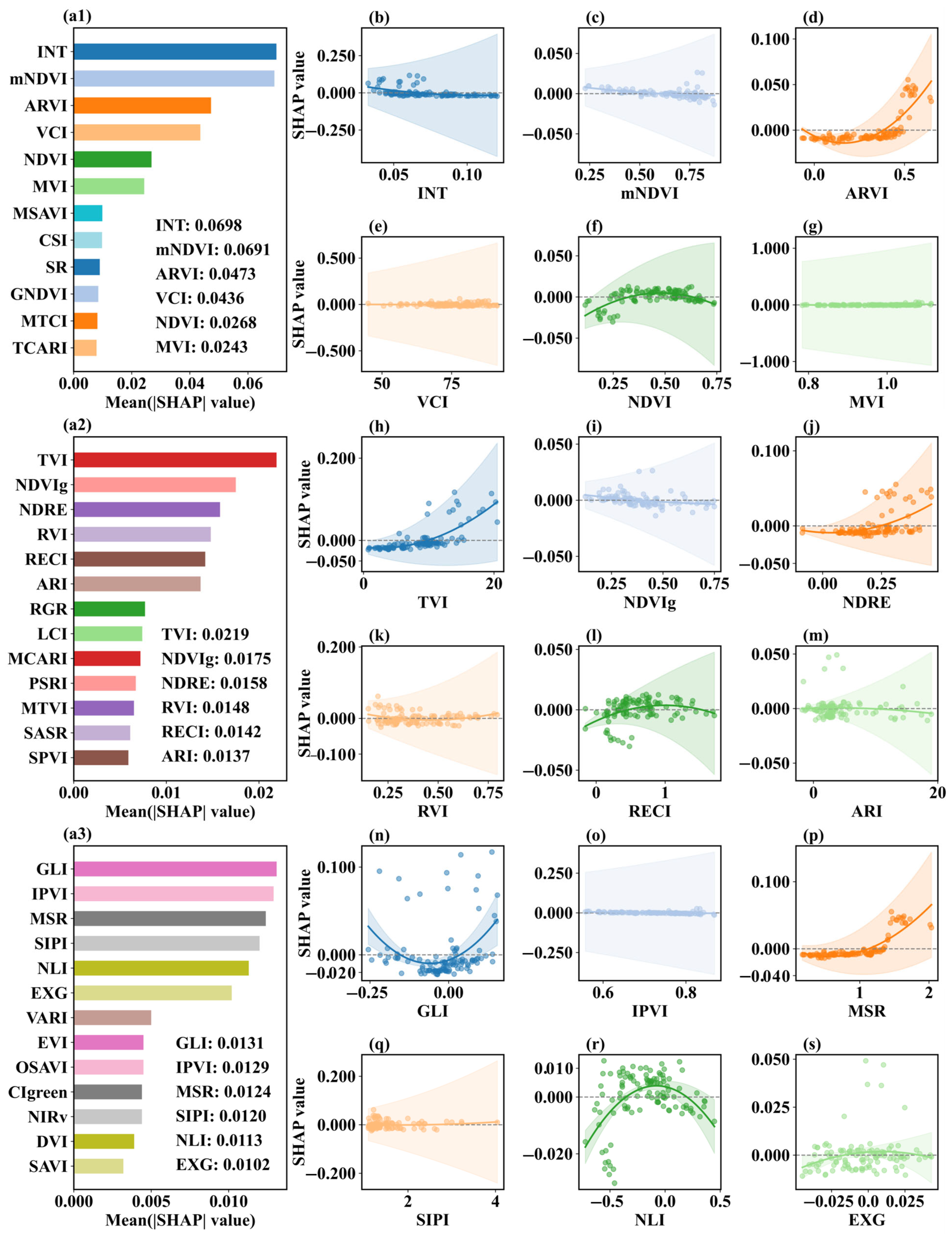
For VI-only LAI retrieval, VIs with a mean absolute SHAP value > 0.01 were retained to ensure informational sufficiency and model parsimony for LAI retrieval (Figure 5a1–a3). The screening determined by this threshold yielded 18 candidate features: INT, mNDVI, ARVI, VCI, NDVI, MVI, TVI, NDVIg, NDRE, RVI, RECI, ARI, GLI, IPVI, MSR, SIPI, NLI and EXG. SHAP partial dependence plots (Figure 5b–s) further exhibit the nonlinear contribution patterns of these VIs to LAI prediction. Each plot quantifies the relationship between VI values and their predictive impact.

Figure 5.
SHAP-based analysis of VIs for LAI retrieval: (a1–a3) show the mean absolute SHAP values of VIs (INT, mNDVI, ARVI, VCI, NDVI, MVI, TVI, NDVIg, NDRE, RVI, RECI, ARI, GLI, IPVI, MSR, SIPI, NLI and EXG) derived from three machine learning models. Each scatter plot (b–s) shows the SHAP partial dependence relationships of the selected VIs. The solid line reflects the overall contribution trend, and the shaded area represents the 95% confidence interval. Positive SHAP values indicate a promotional effect on LAI prediction, while negative values indicate the inverse.
INT shows a positive contribution to LAI prediction at low values, and the curve gradually levels off as INT increases, suggesting a stable contribution. mNDVI exhibits a negative effect on LAI in the high-value range but a clear positive and stable effect in the low-value range. ARVI exhibits a pronounced nonlinear relationship, with substantially enhanced predictive contributions at higher values. Overall, these scatter plots reveal the direction, strength, and potential nonlinear effects of different indices on LAI prediction.
3.2.2. Key PCF Selection with Mean Absolute SHAP Values
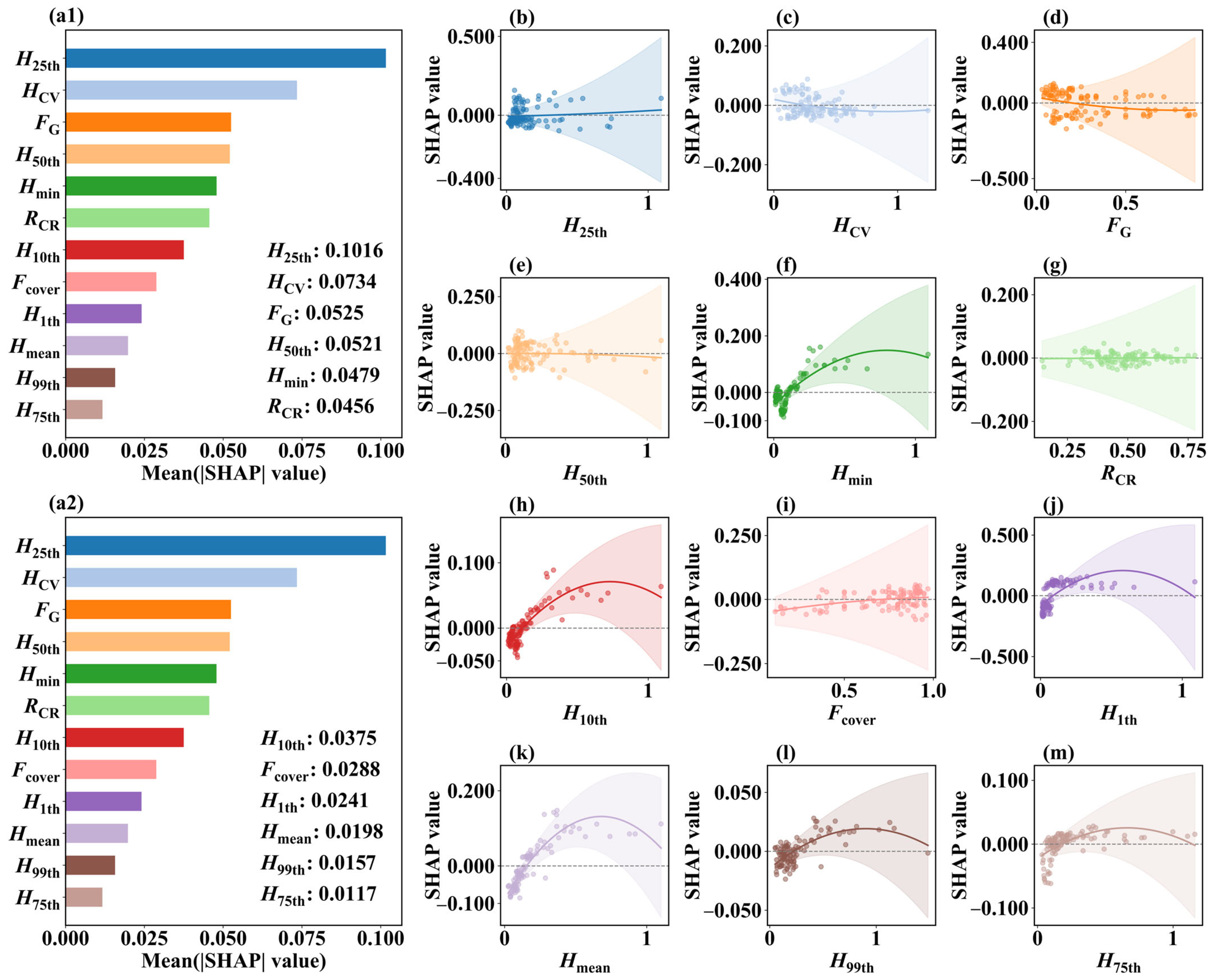
With the same threshold, 12 candidate PCFs were selected: H25th, HCV, FG, H50th, Hmin, RCR, H10th, Fcover, H1th, Hmean, H99th, and H75th (Figure 6a1,a2). Similarly, the scatterplots in Figure 6b–m illustrate the SHAP partial dependence relationships of the preliminarily selected PCFs. H25th exhibits a clear positive contribution trend as its value increases, indicating that a greater lower-canopy height consistently enhances LAI prediction capability. HCV and FG contribute the most strongly to LAI prediction in the low-value range, revealing that canopy height variability and vegetation cover can enhance predictive ability within certain ranges, although their influence becomes limited at higher values. These structural parameters, therefore, reflect canopy density and spatial configuration from different perspectives, providing complementary information for model prediction.
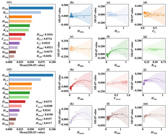
Figure 6.
SHAP-based analysis of PCFs for LAI retrieval: (a1,a2) show the relative importance of PCFs in LAI prediction, quantified by mean absolute SHAP values. (b–m) depict the SHAP partial dependence plots of the selected PCFs (H25th, HCV, FG, H50th, Hmin, RCR, H10th, Fcover, H1th, Hmean, H99th, and H75th). Each scatter point denotes the value of a PCF and its associated SHAP value; the solid line reflects the overall contribution trend, and the shaded area represents the 95% confidence interval.
3.2.3. Fused Feature Screening with Mean Absolute SHAP Values
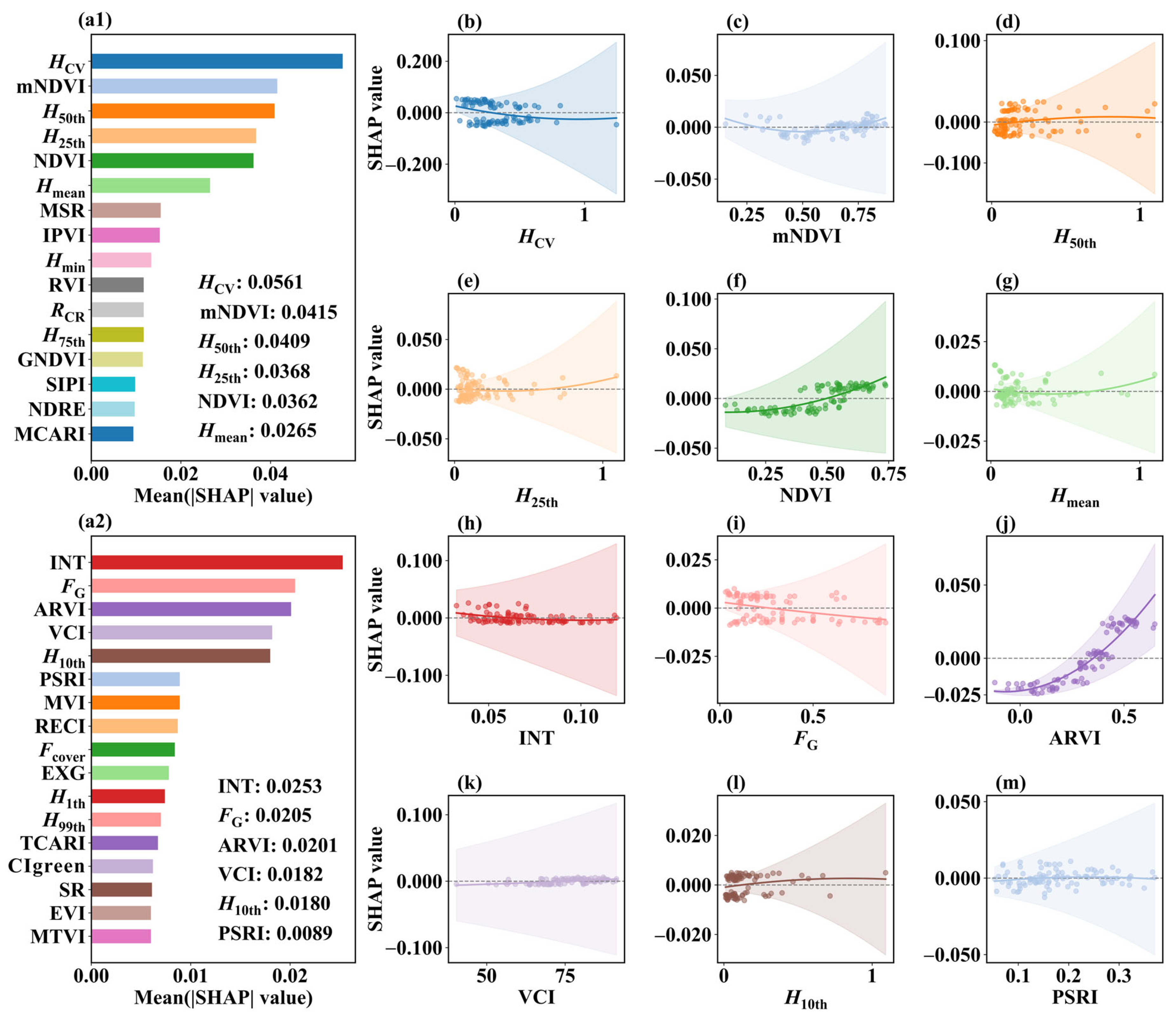
For the fused features, a threshold of a mean absolute SHAP value greater than 0.018 was chosen to identify key variables. This threshold was determined experimentally by comparing the model performance with different SHAP value thresholds (0.05, 0.04, 0.03, 0.02, 0.018, and 0.01). Features with SHAP values greater than or equal to 0.018 were found to contribute most significantly to the model’s performance, as demonstrated through performance comparison (R2 and RMSE) across three models (RF, XGBoost, and CatBoost). This led to the selection of 11 candidate features: HCV, mNDVI, H50th, H25th, NDVI, Hmean, INT, FG, ARVI, VCI and H10th (Figure 7a1,a2). The SHAP partial dependence relationships of these fused features are shown in Figure 7b–l. Taking representative features as examples, H25th exhibits a markedly enhanced positive contribution to LAI prediction in the high-value range, indicating that lower-percentile canopy heights are sensitive indicators of canopy density changes. INT contributes strongly and positively to LAI in the low-value range, reflecting its sensitivity to vegetation physiological status with low chlorophyll content. In contrast, H50th and H10th contribute most strongly at intermediate values, but their positive effects gradually weaken as they increase. Conversely, mNDVI shows a negative contribution in the medium-value range but a substantially enhanced positive contribution as it increases. The complementary trends of VIs and PCFs across different value ranges thus improved the overall predictive capacity of the model for LAI.
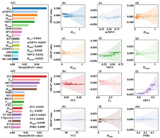
Figure 7.
SHAP analysis of fused features: (a1,a2) illustrate the relative importance of fused features in LAI prediction, quantified by mean absolute SHAP values. (b–m) depict the SHAP partial dependence plots of the selected fused features (HCV, mNDVI, H50th, H25th, NDVI, Hmean, INT, FG, ARVI, VCI and H10th). Each scatter point denotes the value of a sample fused feature and its associated SHAP value; the solid line reflects the overall contribution trend, and the shaded area represents the 95% confidence interval. Notably, features exhibit nonlinear contribution patterns across value ranges, confirming the complementary roles of spectral (VI-derived) and structural (PCF-derived) features in LAI prediction.
3.2.4. Final Non-Redundant Feature Subsets
After initial SHAP-based screening, highly collinear variables were eliminated based on correlation analysis, while also considering their practical contributions to LAI retrieval and the magnitude of their mean absolute SHAP values. The final feature subsets are summarized in Table 6.

Table 6.
Final non-redundant feature subsets with SHAP–correlation strategy.
For the VI set, nine indices were ultimately retained: INT, mNDVI, VCI, TVI, NDVIg, NDRE, ARI, GLI, and SIPI. For the PCF set, six indices were preserved: FG, HCV, RCR, H25th, H50th, and H99th. For the fused set, seven features were retained: HCV, mNDVI, H50th, H25th, INT, FG, and VCI.
Notably, the fused subset retained seven features but combined the most impactful spectral and structural variables, confirming that the SHAP–correlation strategy effectively removes redundancy while preserving complementary information. This significantly enhanced the model’s ability to identify and differentiate varying LAI levels, thereby providing more reliable feature information for LAI retrieval.
3.3. LAI Retrieval Performance of Different Models
3.3.1. VI-Based Models for LAI Retrieval
Using the retained VIs (INT, mNDVI, VCI, TVI, NDVIg, NDRE, ARI, GLI, and SIPI) as input variables, LAI retrieval models were constructed using the RF, XGBoost, and CatBoost algorithms (Figure 8). The results show that the XGBoost-based model achieved higher accuracy (R2 = 0.735, RMSE = 0.33), outperforming the RF (R2 = 0.521, RMSE = 0.448) and CatBoost models (R2 = 0.622, RMSE = 0.398). However, the XGBoost model exhibited both overestimation and underestimation issues: in the low-LAI range (<1.0), LAI values were significantly overestimated, whereas in the high-LAI range (>2.5), they were underestimated, resulting in an overall LAI error of nearly 40%.

Figure 8.
Accuracy analysis of LAI estimation based on VIs.
3.3.2. PCF-Based Models for LAI Retrieval
Using the selected PCFs (FG, HCV, RCR, H25th, H50th, and H99th) as input features, LAI retrieval models were constructed with the RF, XGBoost, and CatBoost algorithms, with subsequent quantitative accuracy validation and comparative analysis (Figure 9). The results show that the RF model achieved the highest accuracy (R2 = 0.894, RMSE = 0.208), which was significantly better than the XGBoost (R2 = 0.800, RMSE = 0.286) and CatBoost models (R2 = 0.782, RMSE = 0.299). Notably, the RF model based on PCFs yielded an overall relative LAI retrieval error of approximately 20%, which was lower than that of the VI-only LAI retrieval models. Specifically, this PSC-based RF model retrieved canopy structural information with higher efficacy in the low-to-medium LAI range, effectively mitigating the overestimation bias of VI-only models in low-LAI zones (<1.0) and the underestimation bias in high-LAI zones (>2.5).

Figure 9.
Accuracy analysis of LAI estimation based on PCFs.
3.3.3. Fused Feature-Based Models for LAI Retrieval
Using the selected fused features (HCV, mNDVI, H50th, H25th, INT, FG, and VCI) as input features, LAI retrieval models were constructed with RF, XGBoost, and CatBoost algorithms, followed by accuracy validation and comparative analysis (Figure 10). The results show that the overall LAI retrieval accuracy of these models based on fused features was significantly higher than that of single-feature models (VI-only or PCF-only) (Table 7). Specifically, compared with the PCF-based model, the RF, XGBoost, and CatBoost models exhibited improvements of 0.074, 0.162, and 0.167 in R2 and reductions of 8.3%, 15%, and 14% in RMSE, respectively.

Figure 10.
Accuracy analysis of LAI estimation based on fused features.

Table 7.
Comparison of model performance.
Among the three algorithms, the RF model based on fused features exhibited the optimal LAI retrieval performance on the independent testing set (R2 = 0.968, RMSE = 0.125). To assess the model’s stability and generalization ability, five-fold cross-validation was implemented. The results show a mean R2 score of 0.726 with a standard deviation of 0.0356, indicating that the model performs consistently across different data partitions despite some variability due to the limited sample size.
The fused features effectively mitigated the underestimation issue of VIs in the high-LAI range while retaining the structural sensitivity of PCFs in canopies. Notably, although the number of fused features was relatively small, PCFs substantially contributed to the fusion model (Figure 7), providing key descriptions of canopy vertical distribution and structural differences. This ensured stable model performance across a full LAI gradient and significantly improved the accuracy of wetland vegetation LAI retrieval.
3.4. Spatial Distribution of Wetland Vegetation LAI
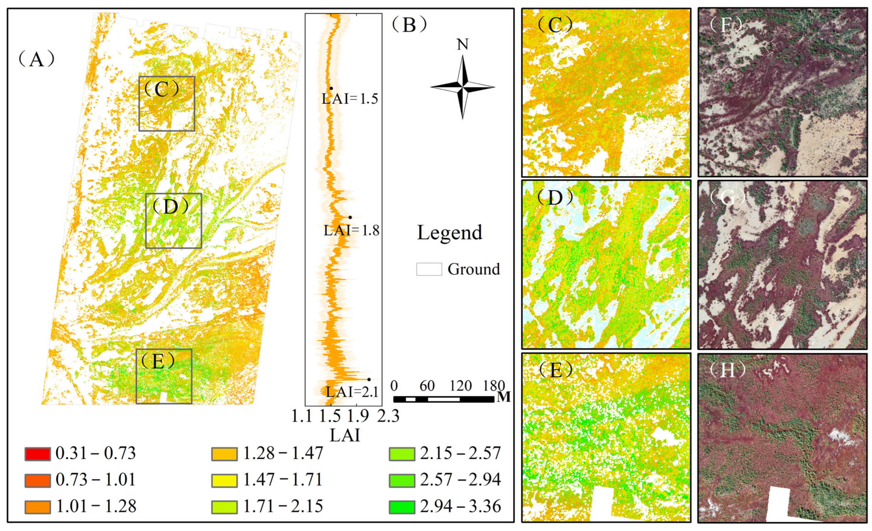
After comparing the accuracy of different models, the RF model based on the fusion of VIs and PCFs was selected as the optimal model to retrieve vegetation LAI across the study area (Figure 11A). The results show that the spatial distribution of LAI exhibited pronounced heterogeneity, with distinct regional differences. In addition, in this map, LAI was predicted only for vegetated pixels after applying a non-vegetation mask (including open water). The water bodies shown in Figure 11A are overlaid only for background visualization and do not represent LAI values.
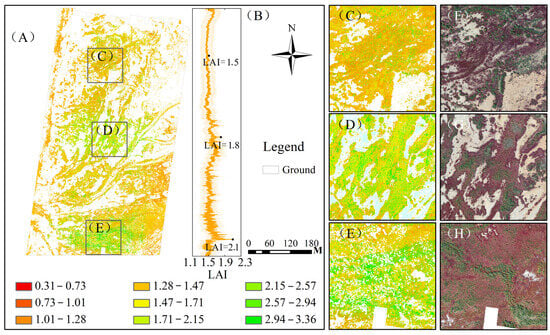
Figure 11.
Spatial distribution of LAI: (A) illustrates the overall LAI spatial pattern; (B) depicts the LAI profile (exhibiting an upward trend from top to bottom) calculated from the average LAI of each horizontal row in the entire study area; (C,F) correspond to a selected sub-region and its RGB image, respectively, identifying Suaeda salsa as the dominant vegetation type (associated with low LAI); (D,G) represent a second sub-region and its RGB image, revealing a mixed community of Suaeda salsa and Tamarix chinensis (serving as a transitional zone with slightly elevated LAI); (E,H) denote a third sub-region and its RGB image, showing mixed vegetation of Tamarix chinensis and Phragmites australis (corresponding to the highest LAI values).
The vegetation LAI in the study area exhibited significant fluctuations with an increasing trend from the coastal zone toward the inland region (Figure 11B). In the coastal zone, where tidal inundation and high salinity stress prevail, vegetation was dominated by the salt-tolerant vegetation Suaeda salsa (Figure 11C,F), with relatively low LAI values (0.31–1.47). As the distance from the coast increased, the coastal–inland transitional zone exhibited a gradual decreasing trend in soil salinity, corresponding to a mixed vegetation community dominated by the semi-salt-tolerant deciduous shrub Tamarix chinensis and residual patches of Suaeda salsa (Figure 11D,G), where LAI increased to 1.47–2.57. In the inland desalination zone, where tidal influence was minimal, soil salinity decreased significantly and freshwater availability became more consistent, favoring a vegetation community dominated by tall graminoids (Phragmites australis) coexisting with Tamarix chinensis (Figure 11E,H). Consequently, LAI values in this zone exhibited a further increase, ranging from 2.57 to 3.36.
4. Discussion
4.1. Synergistic Mechanisms of Hyperspectral–LiDAR Fusion for LAI Retrieval
This study clearly demonstrated that the fusion of VIs and PCFs significantly improved the accuracy of wetland vegetation LAI retrieval (RF model training set: R2 = 0.968, RMSE = 0.125), providing strong evidence for the synergistic advantage of combining “spectral + structural” features. Hyperspectral vegetation indices (e.g., mNDVI, INT and VCI) effectively captured spectral traits, which is consistent with the conclusion that vegetation indices are sensitive to LAI [15]. Meanwhile, PCFs (HCV, H50th, H25th, and FG) accurately characterized canopy height percentiles and vertical heterogeneity, compensating for the limitations of spectral data in representing complex canopy structures. This was particularly effective in alleviating overestimation and underestimation issues in low- and high-LAI ranges, respectively, in line with Wang and Fang [10], who successfully estimated LAI using LiDAR-derived structural parameters such as gap fraction and contact frequency. By integrating VIs and PCFs, the model was able to capture both physiological and structural characteristics of vegetation simultaneously, which markedly reduced the limitations of single-source data, especially in ecologically heterogeneous zones such as wetland transition areas.
SHAP–correlation feature selection strategy further elucidated the roles of key variables. In the fusion model, LiDAR-derived HCV, H50th, H25th, and FG made prominent contributions, underscoring the structural influence of canopy vertical stratification on LAI. Among the spectral indices, the high importance of mNDVI, INT, and VCI indicates that capturing vegetation spectral characteristics and color intensity is crucial for LAI retrieval in saline wetland environments. These differentiated contributions provide a quantitative rationale for improving LAI retrieval accuracy in complex wetland settings through the fusion of hyperspectral and LiDAR features [46].
4.2. Role of SHAP–Correlation Selection in Model Accuracy
Strategies with feature selection using different absolute SHAP values had a significant impact on both the accuracy and stability of LAI retrieval (Table 8). We compared two feature selection criteria: (1) absolute SHAP values derived from a single machine learning model (i.e., RF, XGBoost, or CatBoost individually) and (2) mean absolute SHAP values aggregated across the three models. The results revealed that the feature variables selected based on these two criteria exhibited considerable discrepancies, particularly in terms of feature composition and importance ranking.

Table 8.
Comparison of model performance based on feature selection using absolute SHAP values from a single model.
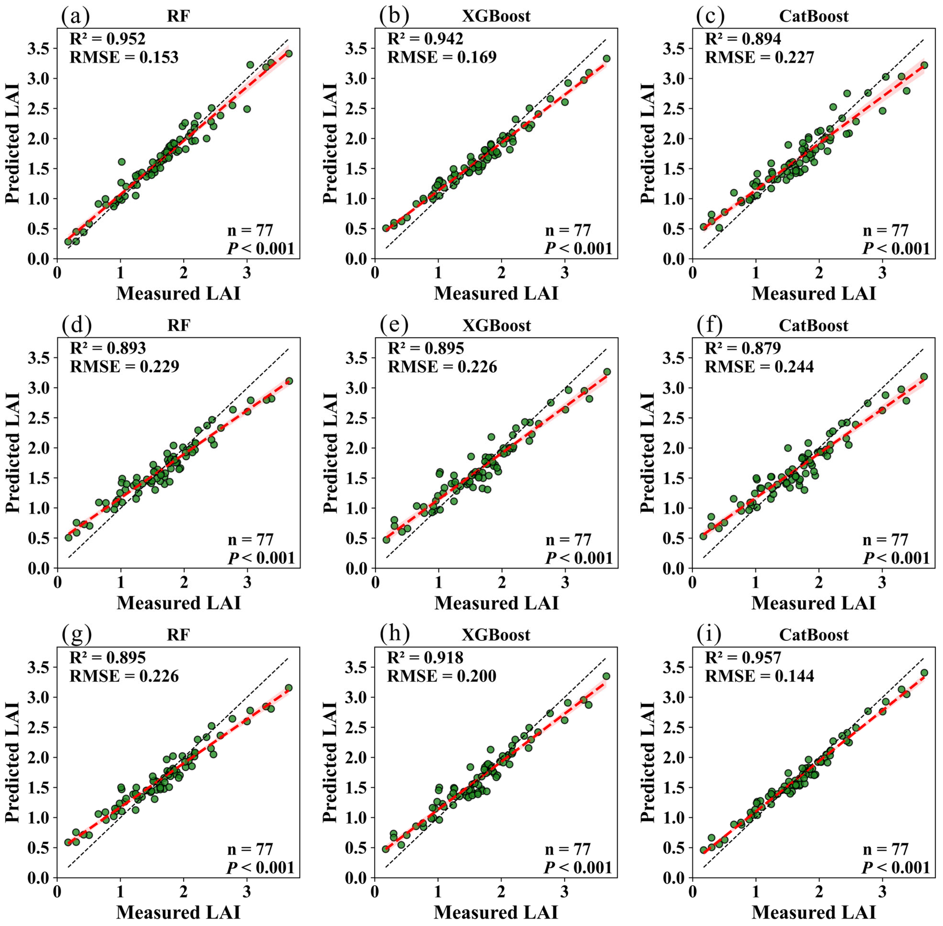
Specifically, when absolute SHAP values derived from a single model were used as the selection reference, the retrieved LAI accuracy of the selected features varied significantly across different LAI inversion models (Figure 12). For instance, features screened via RF-derived SHAP values performed well (R2 = 0.952, RMSE = 0.153) in the RF retrieval model but exhibited accuracy degradation when applied to the XGBoost or CatBoost models, reflecting the strong model dependence of single-model SHAP-based feature selection.
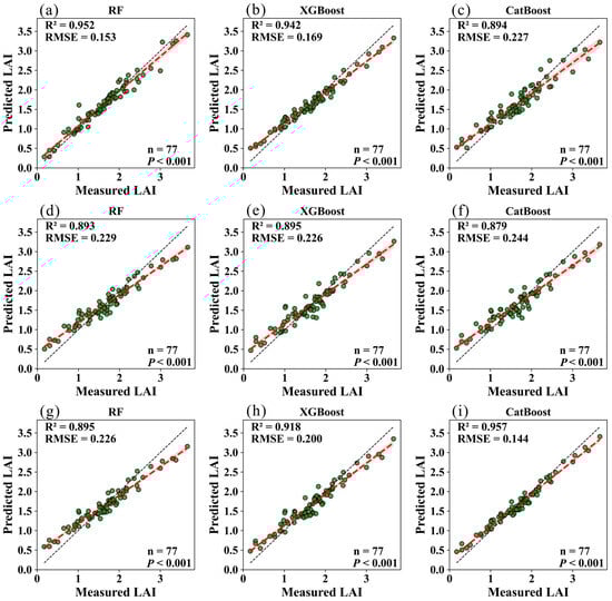
Figure 12.
LAI modeling results based on feature selection using SHAP values from a single model: (a–c) RF model; (d–f) XGBoost model; (g–i) CatBoost model.
In contrast, when mean absolute SHAP values across the three models were adopted as the selection criterion, and strongly collinear features were removed through Pearson analysis, the selected feature variables exhibited better stability across different inversion models, which enabled higher and more stable accuracy across the RF, XGBoost, and CatBoost models, with R2 values of 0.968, 0.962, and 0.949, and RMSE values of 0.125, 0.136, and 0.159, respectively. This stability was attributed to the aggregation of SHAP values mitigating model-specific biases, thereby ensuring the selected features retained robust informational value regardless of the inversion model used.
This result indicates that the feature selection method integrating mean absolute SHAP values with Pearson correlation analysis significantly enhanced the generalization ability and robustness of multi-source features across different machine learning models. This approach yielded greater accuracy advantages, providing a feature selection pathway that balances both precision and robustness for wetland vegetation LAI retrieval.
4.3. Ecological Implication of LAI Spatial Gradients
This coastal-to-inland LAI gradient (0.31–3.36) reflects a typical vegetation successional sequence in estuarine wetlands, including pioneer halophytic herbs (Suaeda salsa), salt-tolerant shrubs (Tamarix chinensis), and freshwater wetland graminoids (Phragmites australis). This spatial distribution pattern of vegetation in Yellow River Delta wetland is highly consistent with the findings reported by Xu et al. [47]: high-salinity plots are dominated by Suaeda salsa and Tamarix chinensis, while low-salinity plots are dominated by Phragmites australis.
In the coastal zone of the study area, subjected to frequent tidal activity and characterized by high soil salinity, Suaeda salsa dominates the vegetation community with relatively low LAI values (Table 2). Subsequently, along the coastal-to-inland vegetation gradient, diminishing tidal influence and decreasing soil salinity drive a shift in community composition; a mixed community of Suaeda salsa and Tamarix chinensis becomes dominant. Corresponding to reduced environmental stress, LAI values exhibit a gradual increasing trend. Finally, in the inland zone with minimal tidal influence, Phragmites australis and Tamarix chinensis gradually replace Suaeda salsa as the dominant vegetation community, supported by stable freshwater availability and low soil salinity. In this zone, LAI values reach relatively high levels (>2.57), facilitated by the dense canopy structure of Phragmites australis.
The fusion features (VIs + PCFs) effectively captured this spatial heterogeneity in LAI from hyperspectral information and characterized canopy structure. These findings are consistent with those of Fang et al. [14], who demonstrated that “habitat gradients drive spatial heterogeneity of vegetation parameters” in Spartina alterniflora wetlands. Consequently, the predicted LAI values not only validate the reliability of the fused features but also provide a quantitative basis for supporting coastal-to-inland vegetation succession monitoring and water–salt regulation in the Yellow River Delta wetlands.
From a practical management perspective, the mapped LAI gradient can be used in several concrete ways. First, it provides an intuitive spatial framework for delineating management zones along the coastal-to-inland transition (e.g., high-stress coastal belt, transitional belt, and relatively stable inland belt), which is useful for designing zonal monitoring schemes and optimizing long-term sampling layouts in a hydrologically controlled estuarine wetland system [48]. Second, persistently low-LAI patches, especially in the frequently tidally disturbed and high-salinity coastal areas, can be treated as priority targets for field inspection and restoration planning, because low vegetation cover and degradation in the Yellow River Delta salt marshes have been repeatedly highlighted as key concerns in recent remote sensing-based monitoring studies [49,50]. Third, repeated LAI mapping can serve as a quantitative indicator with which to evaluate the effectiveness of water–salt regulation or restoration actions by tracking whether low-LAI areas shrink and whether LAI increases in transitional zones after interventions, which aligns with the broader practice of using remote sensing indicators to support restoration monitoring and adaptive management [51]. Finally, because LAI is closely linked to canopy functioning in tidal wetlands and is widely used in productivity and blue carbon-related assessments, documenting LAI gradients and their temporal changes can provide additional ecological context when interpreting management outcomes [52].
4.4. Differences in Model Performance
In this study, the RF model achieved the highest predictive accuracy among the tested algorithms (R2 = 0.968). A plausible reason is that RF is inherently robust to complex nonlinear relationships and noisy predictors thanks to its bootstrap aggregating approach and the averaging of multiple deep decision trees. RF’s structure reduces variance and helps stabilize model predictions, particularly when the sample size is limited or when features are moderately correlated, which is consistent with observations in similar remote sensing applications where RF maintains strong performance across datasets with diverse characteristics [53].
The XGBoost model also achieved high R2 (0.962) but exhibited marginal over- and under-prediction tendencies at the extremes of the LAI range. This behavior may reflect the boosting algorithm’s sensitivity to residual patterns and data distribution skewness. Gradient boosting methods such as XGBoost sequentially fit trees to residual errors and rely on parameter tuning (e.g., learning rate, tree depth) to avoid overfitting and instability; when strong nonlinear interactions exist, the boosting procedure may require careful regularization to achieve optimal balance between fitting training data and generalizing to unseen cases [54].
The CatBoost model performed slightly lower (R2 = 0.949) relative to RF and XGBoost in this study. CatBoost was designed to handle categorical features more efficiently and reduce prediction bias with ordered boosting; however, in regression tasks dominated by fully continuous spectral and structural predictors (e.g., VIs and PCFs), CatBoost’s advantages with categorical handling may be less relevant. This performance trend is supported by comparative studies showing that no single tree-based ensemble consistently dominates across all data types and that model performance can depend on the nature of the input variables and tuning strategy [55].
Together, these findings emphasize that, while tree ensemble methods generally yield strong predictive capability for remote sensing-derived LAI estimation, subtle differences in algorithmic mechanisms (bagging vs. boosting, handling of noise and feature types, regularization strategies) can influence prediction accuracy and behavior across different portions of the target range.
4.5. Limitations and Future Perspectives
This study has some limitations. First, the sample size was relatively small, and data collection was concentrated in September, failing to capture seasonal LAI dynamics across the entire growing season, which may have limited the model’s adaptability to phenological variations [16]. Second, the feature selection criterion (mean absolute SHAP > 0.018 for the fused model) was empirically determined without multi-scale validation, and SHAP-based rankings may vary with model choice and training data, which can influence which predictors are retained [56]. To reduce this effect, we computed SHAP using RF, XGBoost, and CatBoost, screened features based on the mean absolute SHAP across the three models, and interpreted the SHAP results mainly at the feature group level (VIs vs. PCFs) to avoid over-interpreting one predictor within a highly correlated set. Third, the model lacked the integration of environmental covariates (e.g., soil moisture, salinity), whose indirect effects on LAI may not have been fully captured, potentially preventing the model from reflecting true vegetation growth conditions [57]. Fourth, although the hyperspectral and LiDAR data were acquired on the same days and within a short time interval (less than 30 min) under clear-sky and light-wind conditions, residual differences in solar illumination and wind-induced canopy motion may still have introduced uncertainty into the fused features. For passive UAV hyperspectral imagery, even small changes in solar zenith angle, diffuse–direct irradiance ratio, or thin cloud cover can alter surface reflectance and vegetation indices independently of true LAI changes [58,59,60]. Wind-driven canopy movement between the hyperspectral and LiDAR flights may also cause sub-meter geometric mismatches between spectral and structural features, adding noise to the feature-level fusion [61].
To address these limitations, future work will focus on the following aspects: (1) We will expand the sample size and design multi-temporal UAV imagery and field measurement experiments that cover key phenological stages (spring green-up, summer vigorous growth, and autumn senescence) so that the SHAP–correlation feature selection and fusion framework can be extended to build phenology-integrated dynamic LAI retrieval models and to evaluate the seasonal stability of model performance. (2) We will introduce more data-driven feature selection and threshold-setting procedures (e.g., Bayesian optimization) to reduce the subjectivity of the SHAP-based screening criterion [62] and check the stability of selected features across different base models (RF, XGBoost, and CatBoost). This approach will help optimize feature selection thresholds and ensure the robustness of feature subsets across different spatial and temporal conditions by leveraging multi-scale validation. (3) We will integrate environmental data such as soil salinity and water level with remote sensing data to establish innovative retrieval framework [57], thereby further improving the accuracy and generalization of wetland LAI estimation. Also, (4) we will explicitly address these illumination- and motion-related uncertainties by (1) applying BRDF (Bidirectional Reflectance Distribution Function) and illumination normalization schemes to the UAV hyperspectral imagery, such as kernel-driven or flexible BRDF approaches [60,63]; (2) testing LiDAR-assisted radiometric normalization strategies that use calibrated LiDAR intensity to compensate for shadows and illumination gradients in the hyperspectral data [64]; and (3) further reducing the temporal gap between hyperspectral and LiDAR acquisitions and exploring motion compensation and advanced co-registration procedures for UAV imagery acquired under windy conditions [61].
5. Conclusions
This study focused on wetland vegetation LAI retrieval in the Yellow River Delta, coupling UAV-borne hyperspectral imagery and LiDAR point cloud data and using three machine learning algorithms—RF, XGBoost, and CatBoost—to assess the utility of multi-source remote sensing data for LAI retrieval. The main conclusions are summarized as follows:
- Multi-source remote sensing data fusion substantially improves LAI retrieval accuracy. Models dependent on hyperspectral-derived VIs or LiDAR-derived PCFs showed inherent limitations. In contrast, the integration of fused features markedly enhanced model performance and achieved consistently high accuracy results across different algorithms. Notably, the RF model had better performance, attaining R2 = 0.968 and RMSE = 0.125.
- The feature screening strategy exerts a pivotal influence on modeling robustness. The feature selection strategy aggregated the mean absolute SHAP values across the three models, yielding higher and stabler LAI retrieval accuracy. This advantage stems from the aggregated SHAP method to mitigate model-specific biases and retain features with robust informational value, thereby enhancing the ability of LAI retrieval models across different algorithmic frameworks.
- Critical predictive variables for wetland LAI retrieval are identified. Combined Pearson correlation analysis and SHAP value analysis indicated that PCFs (HCV, H50th, H25th, and FG) and VIs (mNDVI, INT, and VCI) significantly contributed to accurate LAI retrieval.
- Wetland LAI exhibits significant fluctuations from the coastal zone to the inland region, with a tendency for increasing values. This spatial trend of LAI in the study area was consistent with the distribution of wetland vegetation and the gradient changes in growth environments. The fused features effectively capture this heterogeneity, validating the fusion model’s capacity to resolve ecologically meaningful spatial patterns in wetland vegetation LAI.
Author Contributions
Conceptualization, J.W. and C.S.; methodology, J.W., T.C. and J.D.; software, Y.M. and X.Y.; validation, C.S. and T.C.; formal analysis, C.S.; investigation, C.S., X.J. and H.L.; data curation, X.J., X.Y. and H.L.; writing—original draft preparation, C.S.; writing—review and editing, J.W., S.Q. and T.C.; visualization, C.S., J.D. and S.Q.; supervision, Y.M. and F.G.; project administration, J.W., Y.M. and F.G.; funding acquisition, J.W., S.Q., X.J. and J.D. All authors have read and agreed to the published version of the manuscript.
Funding
This research was funded by the National Natural Science Foundation of China (Grant no. 4230144), Joint Fund of Henan Province Science and Technology R&D Program (Grant no. 225200810057), Science and Technology Project of Henan Province (Grant no. 252102321108), The Innovation Team Project of Henan Academy of Sciences (Grant no. 20230107), The “Double First-Class” Discipline Construction Project of Surveying and Mapping Science and Technology, Henan Polytechnic University (Grant no. GCCYJ202401), Henan Provincial Natural Science Foundation for General Program (Grant no. 242300421365) and Humanities and Social Sciences Research Project of the Henan Provincial Department of Education (Grant no. 2024-ZZJH-147).
Data Availability Statement
The datasets used and analyzed during the current study are available from the corresponding author on reasonable request.
Conflicts of Interest
The authors declare no conflicts of interest.
References
- Ferreira, C.S.; Kašanin-Grubin, M.; Solomun, M.K.; Sushkova, S.; Minkina, T.; Zhao, W.; Kalantari, Z. Wetlands as nature-based solutions for water management in different environments. Curr. Opin. Environ. Sci. Health 2023, 33, 100476. [Google Scholar] [CrossRef]
- Fang, H.; Baret, F.; Plummer, S.; Schaepman-Strub, G. An overview of global leaf area index (LAI): Methods, products, validation, and applications. Rev. Geophys. 2019, 57, 739–799. [Google Scholar] [CrossRef]
- Parker, G.G. Tamm review: Leaf Area Index (LAI) is both a determinant and a consequence of important processes in vegetation canopies. For. Ecol. Manag. 2020, 477, 118496. [Google Scholar] [CrossRef]
- Lu, L.; Luo, J.; Xin, Y.; Duan, H.; Sun, Z.; Qiu, Y.; Xiao, Q. How can UAV contribute in satellite-based Phragmites australis aboveground biomass estimating? Int. J. Appl. Earth Obs. Geoinf. 2022, 114, 103024. [Google Scholar] [CrossRef]
- Ali, A.M.; Darvishzadeh, R.; Skidmore, A.; Gara, T.W.; O’Connor, B.; Roeoesli, C.; Paganini, M.; Heurich, M.; Paganini, M. Comparing methods for mapping canopy chlorophyll content in a mixed mountain forest using Sentinel-2 data. Int. J. Appl. Earth Obs. Geoinf. 2020, 87, 102037. [Google Scholar] [CrossRef]
- Wang, Q.; Tang, Y.; Ge, Y.; Xie, H.; Tong, X.; Atkinson, P.M. A comprehensive review of spatial-temporal-spectral information reconstruction techniques. Sci. Remote Sens. 2023, 8, 100102. [Google Scholar] [CrossRef]
- Jin, H.; Qiao, Y.; Liu, T.; Xie, X.; Fang, H.; Guo, Q.; Zhao, W. A hierarchical downscaling scheme for generating fine-resolution leaf area index with multisource and multiscale observations via deep learning. Int. J. Appl. Earth Obs. Geoinf. 2024, 133, 104152. [Google Scholar] [CrossRef]
- Li, C.; Zhou, H.; Tang, J.; Wang, C.; Wang, Z.; Qi, J.; Yang, B.; Fang, R. Time-series high spatio-temporal resolution vegetation leaf area index estimation based on NDVI trends. Int. J. Appl. Earth Obs. Geoinf. 2025, 142, 104744. [Google Scholar] [CrossRef]
- Yan, P.; Feng, Y.; Han, Q.; Hu, Z.; Huang, X.; Su, K.; Kang, S. Enhanced cotton chlorophyll content estimation with UAV multispectral and LiDAR constrained SCOPE model. Int. J. Appl. Earth Obs. Geoinf. 2024, 132, 104052. [Google Scholar] [CrossRef]
- Wang, Y.; Fang, H. Estimation of LAI with the LiDAR technology: A review. Remote Sens. 2020, 12, 3457. [Google Scholar] [CrossRef]
- Shi, Z.; Shi, S.; Gong, W.; Xu, L.; Wang, B.; Sun, J.; Xu, Q. LAI estimation based on physical model combining airborne LiDAR waveform and Sentinel-2 imagery. Front. Plant Sci. 2023, 14, 1237988. [Google Scholar] [CrossRef] [PubMed]
- Du, X.Y.; Wan, L.; Cen, H.Y.; Chen, S.B.; Zhu, J.P.; Wang, H.Y.; He, Y. Multi-temporal monitoring of leaf area index of rice under different nitrogen treatments using UAV images. Int. J. Precis. Agric. Aviat. 2020, 3, 7–12. [Google Scholar] [CrossRef]
- Liu, S.; Jin, X.; Bai, Y.; Wu, W.; Cui, N.; Cheng, M.; Liu, Y.; Meng, L.; Jia, X.; Nie, C.; et al. UAV multispectral images for accurate estimation of the maize LAI considering the effect of soil background. Int. J. Appl. Earth Obs. Geoinf. 2023, 121, 103383. [Google Scholar] [CrossRef]
- Fang, H.; Man, W.; Liu, M.; Zhang, Y.; Chen, X.; Li, X.; Tian, D. Leaf area index inversion of Spartina alterniflora using UAV hyperspectral data based on multiple optimized machine learning algorithms. Remote Sens. 2023, 15, 4465. [Google Scholar] [CrossRef]
- Liang, L.; Di, L.; Zhang, L.; Deng, M.; Qin, Z.; Zhao, S.; Lin, H. Estimation of crop LAI using hyperspectral vegetation indices and a hybrid inversion method. Remote Sens. Environ. 2015, 165, 123–134. [Google Scholar] [CrossRef]
- Liang, L.; Geng, D.; Yan, J.; Qiu, S.; Di, L.; Wang, S.; Li, L. Estimating crop LAI using spectral feature extraction and the hybrid inversion method. Remote Sens. 2020, 12, 3534. [Google Scholar] [CrossRef]
- Yang, J.; Xing, M.; Tan, Q.; Shang, J.; Song, Y.; Ni, X.; Wang, J.; Xu, M. Estimating effective leaf area index of winter wheat based on UAV point cloud data. Drones 2023, 7, 299. [Google Scholar] [CrossRef]
- Norton, C.L.; Hartfield, K.; Collins, C.D.H.; van Leeuwen, W.J.; Metz, L.J. Multi-temporal LiDAR and hyperspectral data fusion for classification of semi-arid woody cover species. Remote Sens. 2022, 14, 2896. [Google Scholar] [CrossRef]
- Wang, B.; Liu, J.; Li, J.; Li, M. UAV LiDAR and hyperspectral data synergy for tree species classification in the Maoershan Forest Farm region. Remote Sens. 2023, 15, 1000. [Google Scholar] [CrossRef]
- Ma, Y.; Zhao, Y.; Im, J.; Zhao, Y.; Zhen, Z. A deep-learning-based tree species classification for natural secondary forests using unmanned aerial vehicle hyperspectral images and LiDAR. Ecol. Indic. 2024, 159, 111608. [Google Scholar] [CrossRef]
- Xu, Y.; Qin, Y.; Li, B.; Li, J. Estimating vegetation aboveground biomass in Yellow River Delta coastal wetlands using Sentinel-1, Sentinel-2 and Landsat-8 imagery. Ecol. Inform. 2025, 87, 103096. [Google Scholar] [CrossRef]
- Gao, S.; Yan, K.; Liu, J.; Pu, J.; Zou, D.; Qi, J.; Mu, X.; Yan, G. Assessment of remote-sensed vegetation indices for estimating forest chlorophyll concentration. Ecol. Indic. 2024, 162, 112001. [Google Scholar] [CrossRef]
- Bannari, A.; Morin, D.; Bonn, F.; Huete, A. A review of vegetation indices. Remote Sens. Rev. 1995, 13, 95–120. [Google Scholar] [CrossRef]
- Kaur, N.; Sharma, A.K.; Shellenbarger, H.; Griffin, W.; Serrano, T.; Brym, Z.; Sharma, L.K. Drone and handheld sensors for hemp: Evaluating NDVI and NDRE in relation to nitrogen application and crop yield. Agrosyst. Geosci. Environ. 2025, 8, e70075. [Google Scholar] [CrossRef]
- Bak, H.J.; Kim, E.J.; Lee, J.H.; Chang, S.; Kwon, D.; Im, W.J.; Kim, D.H.; Lee, I.H.; Lee, M.J.; Hwang, W.H.; et al. Canopy-Level Rice Yield and Yield Component Estimation Using NIR-Based Vegetation Indices. Agriculture 2025, 15, 594. [Google Scholar] [CrossRef]
- Yeom, J.; Jung, J.; Chang, A.; Ashapure, A.; Maeda, M.; Maeda, A.; Landivar, J. Comparison of vegetation indices derived from UAV data for differentiation of tillage effects in agriculture. Remote Sens. 2019, 11, 1548. [Google Scholar] [CrossRef]
- Chen, J.M. Evaluation of vegetation indices and a modified simple ratio for boreal applications. Can. J. Remote Sens. 1996, 22, 229–242. [Google Scholar] [CrossRef]
- Zhu, X.; Li, Q.; Guo, C. Evaluation of the monitoring capability of various vegetation indices and mainstream satellite band settings for grassland drought. Ecol. Inform. 2024, 82, 102717. [Google Scholar] [CrossRef]
- Barati, S.; Rayegani, B.; Saati, M.; Sharifi, A.; Nasri, M. Comparison the accuracies of different spectral indices for estimation of vegetation cover fraction in sparse vegetated areas. Egypt. J. Remote Sens. Space Sci. 2011, 14, 49–56. [Google Scholar] [CrossRef]
- Gitelson, A.A.; Merzlyak, M.N.; Chivkunova, O.B. Optical properties and nondestructive estimation of anthocyanin content in plant leaves. Photochem. Photobiol. 2001, 74, 38–45. [Google Scholar] [CrossRef]
- Kogan, F.N. Application of vegetation index and brightness temperature for drought detection. Adv. Space Res. 1995, 15, 91–100. [Google Scholar] [CrossRef]
- Gamon, J.A.; Surfus, J.S. Assessing leaf pigment content and activity with a reflectometer. New Phytol. 1999, 143, 105–117. [Google Scholar] [CrossRef]
- Meng, L.; Yin, D.; Cheng, M.; Liu, S.; Bai, Y.; Liu, Y.; Jin, X. Improved crop biomass algorithm with piecewise function (iCBA-PF) for maize using multi-source UAV data. Drones 2023, 7, 254. [Google Scholar] [CrossRef]
- Badgley, G.; Field, C.B.; Berry, J.A. Canopy near-infrared reflectance and terrestrial photosynthesis. Sci. Adv. 2017, 3, e1602244. [Google Scholar] [CrossRef] [PubMed]
- Sims, D.A.; Gamon, J.A. Relationships between leaf pigment content and spectral reflectance across a wide range of species, leaf structures and developmental stages. Remote Sens. Environ. 2002, 81, 337–354. [Google Scholar] [CrossRef]
- Pu, R.; Gong, P.; Yu, Q. Comparative analysis of EO-1 ALI and Hyperion, and Landsat ETM+ data for mapping forest crown closure and leaf area index. Sensors 2008, 8, 3744–3766. [Google Scholar] [CrossRef]
- Metternicht, G. Vegetation indices derived from high-resolution airborne videography for precision crop management. Int. J. Remote Sens. 2003, 24, 2855–2877. [Google Scholar] [CrossRef]
- Main, R.; Cho, M.A.; Mathieu, R.; O’Kennedy, M.M.; Ramoelo, A.; Koch, S. An investigation into robust spectral indices for leaf chlorophyll estimation. ISPRS J. Photogramm. Remote Sens. 2011, 66, 751–761. [Google Scholar] [CrossRef]
- Huete, A.R. A soil-adjusted vegetation index (SAVI). Remote Sens. Environ. 1998, 25, 295–309. [Google Scholar] [CrossRef]
- Jiang, Z.; Huete, A.R.; Kim, Y.; Didan, K. 2-band enhanced vegetation index without a blue band and its application to AVHRR data. In Remote Sensing and Modeling of Ecosystems for Sustainability IV; SPIE: Bellingham, MA, USA, 2007; Volume 6679, pp. 45–53. [Google Scholar]
- Tahir, M.N.; Naqvi, S.Z.A.; Lan, Y.B.; Zhang, Y.L.; Wang, Y.K.; Afzal, M.; Cheema, M.J. Real time estimation of chlorophyll content based on vegetation indices derived from multispectral UAV in the kinnow orchard. Int. J. Precis. Agric. Aviat. 2018, 1, 24–31. [Google Scholar] [CrossRef]
- Hanberry, B.B. Practical guide for retaining correlated climate variables and unthinned samples in species distribution modeling, using random forests. Ecol. Inform. 2024, 79, 102406. [Google Scholar] [CrossRef]
- Bradter, U.; Altringham, J.D.; Kunin, W.E.; Thom, T.J.; O’Connell, J.; Benton, T.G. Variable ranking and selection with random forest for unbalanced data. Environ. Data Sci. 2022, 1, e30. [Google Scholar] [CrossRef]
- Bhattarai, D.; Lucieer, A. Random forest regression exploring contributing factors to artificial night-time lights observed in VIIRS satellite imagery. Int. J. Digit. Earth 2024, 17, 2324941. [Google Scholar] [CrossRef]
- Zhang, J.; Cheng, T.; Guo, W.; Xu, X.; Qiao, H.; Xie, Y.; Ma, X. Leaf area index estimation model for UAV image hyperspectral data based on wavelength variable selection and machine learning methods. Plant Methods 2021, 17, 49. [Google Scholar] [CrossRef]
- Mulero, G.; Bonfil, D.J.; Helman, D. Wheat leaf area index retrieval from drone-derived hyperspectral and LiDAR imagery using machine learning algorithms. Agric. For. Meteorol. 2025, 372, 110648. [Google Scholar] [CrossRef]
- Xu, Z.; Li, R.; Dou, W.; Wen, H.; Yu, S.; Wang, P.; Ning, L.; Duan, J.; Wang, J. Plant diversity response to environmental factors in Yellow River delta, China. Land 2024, 13, 264. [Google Scholar] [CrossRef]
- Qiu, M.; Liu, Y.; Chen, P.; He, N.; Wang, S.; Huang, X.; Fu, B. Spatio-temporal changes and hydrological forces of wetland landscape pattern in the Yellow River Delta during 1986–2022. Landsc. Ecol. 2024, 39, 51. [Google Scholar] [CrossRef]
- Chang, D.; Wang, Z.; Ning, X.; Li, Z.; Zhang, L.; Liu, X. Vegetation changes in Yellow River Delta wetlands from 2018 to 2020 using PIE-Engine and short time series Sentinel-2 images. Front. Mar. Sci. 2022, 9, 977050. [Google Scholar] [CrossRef]
- Xu, R.; Fan, Y.; Fan, B.; Feng, G.; Li, R. Classification and Monitoring of Salt Marsh Vegetation in the Yellow River Delta Based on Multi-Source Remote Sensing Data Fusion. Sensors 2025, 25, 529. [Google Scholar] [CrossRef]
- Wang, R.; Sun, Y.; Zong, J.; Wang, Y.; Cao, X.; Wang, Y.; Cheng, X.; Zhang, W. Remote sensing application in ecological restoration monitoring: A systematic review. Remote Sens. 2024, 16, 2204. [Google Scholar] [CrossRef]
- Hawman, P.A.; Mishra, D.R.; O’Connell, J.L. Dynamic emergent leaf area in tidal wetlands: Implications for satellite-derived regional and global blue carbon estimates. Remote Sens. Environ. 2023, 290, 113553. [Google Scholar] [CrossRef]
- Shao, Z.; Ahmad, M.N.; Javed, A. Comparison of random forest and XGBoost classifiers using integrated optical and SAR features for mapping urban impervious surface. Remote Sens. 2024, 16, 665. [Google Scholar] [CrossRef]
- Pawłuszek-Filipiak, K.; Lewandowski, T. The Impact of Feature Selection on XGBoost Performance in Landslide Susceptibility Mapping Using an Extended Set of Features: A Case Study from Southern Poland. Appl. Sci. 2025, 15, 8955. [Google Scholar] [CrossRef]
- Huang, H.; Wu, D.; Fang, L.; Zheng, X. Comparison of multiple machine learning models for estimating the forest growing stock in large-scale forests using multi-source data. Forests 2022, 13, 1471. [Google Scholar] [CrossRef]
- Ding, J.; Du, J.; Wang, H.; Xiao, S. A novel two-stage feature selection method based on random forest and improved genetic algorithm for enhancing classification in machine learning. Sci. Rep. 2025, 15, 16828. [Google Scholar] [CrossRef]
- Luo, Z.; Deng, M.; Tang, M.; Liu, R.; Feng, S.; Zhang, C.; Zheng, Z. Estimating soil profile salinity under vegetation cover based on UAV multi-source remote sensing. Sci. Rep. 2025, 15, 2713. [Google Scholar] [CrossRef] [PubMed]
- Arroyo-Mora, J.P.; Kalacska, M.; Løke, T.; Schläpfer, D.; Coops, N.C.; Lucanus, O.; Leblanc, G. Assessing the impact of illumination on UAV pushbroom hyperspectral imagery collected under various cloud cover conditions. Remote Sens. Environ. 2021, 258, 112396. [Google Scholar] [CrossRef]
- Abdelbaki, A.; Schlerf, M.; Retzlaff, R.; Machwitz, M.; Verrelst, J.; Udelhoven, T. Comparison of Crop Trait Retrieval Strategies Using UAV-Based VNIR Hyperspectral Imaging. Remote Sens. 2021, 13, 1748. [Google Scholar] [CrossRef]
- Jia, W.; Pang, Y.; Tortini, R.; Schläpfer, D.; Li, Z.; Roujean, J.L. A kernel-driven BRDF approach to correct airborne hyperspectral imagery over forested areas with rugged topography. Remote Sens. 2020, 12, 432. [Google Scholar] [CrossRef]
- Lee, K.; Han, X. A study on leveraging unmanned aerial vehicle collaborative driving and aerial photography systems to improve the accuracy of crop phenotyping. Remote Sens. 2023, 15, 3903. [Google Scholar] [CrossRef]
- Zhang, D.; Ni, H. Inversion of forest biomass based on multi-source remote sensing images. Sensors 2023, 23, 9313. [Google Scholar] [CrossRef] [PubMed]
- Queally, N.; Ye, Z.; Zheng, T.; Chlus, A.; Schneider, F.; Pavlick, R.P.; Townsend, P.A. FlexBRDF: A flexible BRDF correction for grouped processing of airborne imaging spectroscopy flightlines. J. Geophys. Res. Biogeosci. 2022, 127, e2021JG006622. [Google Scholar] [CrossRef] [PubMed]
- Brell, M.; Segl, K.; Guanter, L.; Bookhagen, B. Hyperspectral and lidar intensity data fusion: A framework for the rigorous correction of illumination, anisotropic effects, and cross calibration. IEEE Trans. Geosci. Remote Sens. 2017, 55, 2799–2810. [Google Scholar] [CrossRef]
Disclaimer/Publisher’s Note: The statements, opinions and data contained in all publications are solely those of the individual author(s) and contributor(s) and not of MDPI and/or the editor(s). MDPI and/or the editor(s) disclaim responsibility for any injury to people or property resulting from any ideas, methods, instructions or products referred to in the content. |
© 2025 by the authors. Licensee MDPI, Basel, Switzerland. This article is an open access article distributed under the terms and conditions of the Creative Commons Attribution (CC BY) license.

