Satellite-Driven Evaluation of Ecological Environmental Quality Based on the PSR Framework

Highlights

What are the main findings?

• A new remote sensing-based EEQ evaluation indicator system was successfully constructed based on the PSR framework, overcoming the limitations of traditional methods.
• A DNN-based evaluation model was developed and proven effective, achieving more accurate and generally applicable EEQ assessment compared to conventional remote sensing techniques.

What are the implications of the main findings?

• The integration of DNN for data augmentation provides a robust solution to the common challenge of limited samples in remote sensing modeling.
• The spatiotemporal dynamics of EEQ in Guangzhou from 2013 to 2020 were quantitatively revealed, offering critical insights for urban environmental planning and sustainable management.

Abstract

With the intensification of environmental degradation, it is crucial for environmental protection to monitor and evaluate the ecological environmental quality (EEQ) in a timely and accurate manner based on remote sensing technology. However, current remote sensing EEQ evaluation methods suffer from deficiencies with regard to the indicator system and the EEQ quantification, reducing the accuracy of EEQ evaluations. Therefore, a new EEQ evaluation method is proposed in this study. Remote sensing indicators used in the pressure–state–response (PSR) framework are selected based on the traditional EEQ evaluation system, and deep neural networks (DNNs) are used to quantify EEQ. The results show that the proposed method has a significantly higher EEQ estimation accuracy with NRMSE of 13.61% and R² of 0.75 than the commonly used remote sensing ecological index (RSEI) method with NRMSE of 19.13% and R² of 0.51. This study suggests that the proposed method is suitable for the estimation of EEQ in a city.

1. Introduction

The ecological environmental quality (EEQ) has become a major concern of society due to increased environmental pressure caused by resource scarcity, population growth, and urban expansion. The world’s EEQ is facing serious challenges and must be effectively and rapidly monitored and quantified. Traditional EEQ monitoring methods typically use field-measured data and statistical analysis; however, these methods are time-consuming and expensive to derive spatially explicit estimates in a large study [1,2]. Remote sensing (RS) techniques provide an effective tool for the rapid, accurate, and dynamic monitoring and evaluation of EEQ [3].

The current EEQ evaluation methods using RS data can be divided into semi-RS and RS evaluation methods. The semi-RS evaluation method evaluates EEQ using RS data and statistical data based on the traditional EEQ indicator framework. Karimian et al. assessed (EEQ) using conventional EEQ indicators, with the vegetation component derived from remote sensing (RS) data. The results demonstrate that these indicators collectively provide a comprehensive representation of regional EEQ conditions [4]. Mukesh Singh Boori et al. integrated remote sensing data and statistical indicators to construct the Remote Sensing Ecological Index (RSEI) and the Ecological Index (EI) through a weighting scheme. The results demonstrate that both indices are highly comparable in assessing ecological environment quality (EEQ) [5]; however, the EI exhibits superior sensitivity in capturing changes in EEQ. Similar studies have been conducted in India, the United States and other parts of the world [6,7,8]. This semi-RS evaluation method only uses RS data to obtain some of the indicators, whereas others are still derived from traditional statistics and field data, reducing the efficiency of EEQ evaluation.

These indices primarily characterize ecological quality (EQ) by reflecting the intrinsic state of ecosystems, whereas ecological environment quality (EEQ) encompasses a broader connotation that additionally integrates environmental pressures and anthropogenic responses [9]. The RS evaluation method evaluates EEQ using only RS data (e.g., normalized difference vegetation index (NDVI), leaf area index (LAI), and remote sensing ecological index (RSEI)). For example, Cai et al. utilized multi-temporal remote sensing imagery to derive land cover types and vegetation growth status and employed the geographical detector model to analyze the spatial heterogeneity of factors influencing ecological quality. Their results demonstrated that the Remote Sensing Ecological Index (RSEI) can comprehensively and effectively characterize environmental conditions [10]. Wei Z. et al. incorporated the Comprehensive Salinity Index (CSI) and Water Network Density (WND) into ecological quality assessment and developed an RSEI-based model for WND estimation (EMW) [11]. Their findings indicated that RSEI effectively captures surface details in arid regions [12]. Liu Y et al. proposed an enhanced RSEI by integrating five ecological components—vegetation, moisture, dryness, heat, and air quality difference—and demonstrated that the improved model provides a more accurate representation of ground-level ecological conditions [13]. Although these studies have produced valuable outcomes, current RS evaluation methods are rarely integrated with traditional evaluation systems. Most studies used traditional indicators and did not consider other traditional indicators, such as biological abundance and pollution load, resulting in low accuracy of EEQ evaluations. Moreover, these studies evaluated EEQ indirectly by conducting correlation analyses of RS indices but did not quantify EEQ by constructing a model of the relationship between RS indices and EEQ.

The purpose of this study is to design an RS indicator system for evaluating EEQ based on the PSR framework and quantify EEQ using a deep neural network (DNN) algorithm to achieve a rapid and accurate evaluation of EEQ in a large study area. The objectives are to (1) design a remote sensing indicator (RSI) system based on the PSR framework and the traditional indicator system; (2) establish a model describing the relationship between EEQ and RS indicators using DNNs; and (3) map EEQ in a large study area. A case study is conducted in Guangzhou city, Guangdong Province, China, using multi-source RS data (including Landsat 8, the China High particulate matter concentration (PM2.5) dataset, the Global Precipitation Measurement (GPM) satellite precipitation datasets, and the China Land Cover Dataset (CLCD)).

2. Materials and Methods

2.1. Material

2.1.1. Study Area

The study area for creating the optimal EEQ evaluation model was located in Guangdong Province in South China (20.13′–25.31′N and 109.39′–117.19′E), covering an area of about 179,725 km². Guangdong Province has a subtropical monsoon climate characterized by simultaneous rain and heat, sufficient rainfall and sunshine, and low frost and snowfall potential. The mean annual temperature is 21.8 °C, and the mean annual rainfall is 1300–2500 mm. The area has many vegetation types and high vegetation cover. Issues such as habitat fragmentation, vegetation degradation, soil erosion, and the weakening of ecosystem services have become increasingly prominent, thereby contributing to spatially heterogeneous EEQ. Given its pronounced ecological gradients, strong human–environment interactions, and representativeness of typical subtropical ecosystems under rapid development, the EEQ in Guangdong province is changing dynamically due to anthropogenic and environmental factors.

As the provincial capital of Guangdong, Guangzhou City was used for model validation and application analysis. Guangzhou is located in south–central Guangdong Province. The elevation decreases from northeast to southwest, and the terrain is dominated by low mountains and hills. As the provincial capital and a cosmopolitan city, Guangzhou is experiencing rapid economic growth and the expansion of built-up areas, significantly affecting ecosystems. Consequently, a spatiotemporal analysis of the EEQ of the city can be used as an example for other rapidly growing cities and cosmopolitan cities globally.

2.1.2. Data Collection and Pre-Processing

We collected 373 county-scale measurements of EEQ from the Department of Ecology and Environment of Guangdong Province in 2013 (123 plots), 2016 (125 plots), and 2019 (125 plots) (Figure 1). The sample data were randomly divided into two groups: 70% of the samples (blue plots in Figure 1) were used for modeling, and the other 30% (pink plots in Figure 1) were used to evaluate the reliability of the EEQ estimation model. Moreover, 34 measured samples in Guangzhou (pink plots in Figure 2) were used for validating the accuracy of mapping EEQ. The soil type and property data were obtained from Soil Science Datasets.

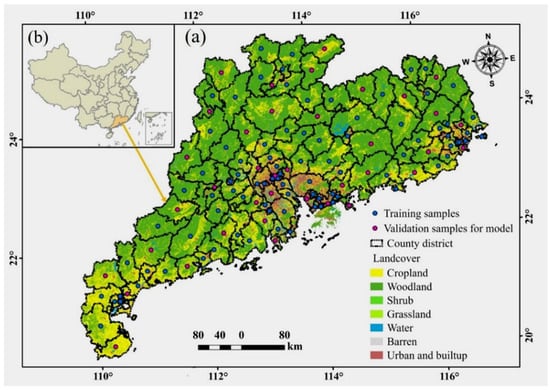
Figure 1. (a) The study area and the 125 sample plots (training samples in blue and validation samples in pink); (b) location of the study area in China.

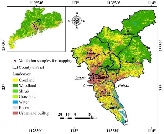
Figure 2. Land cover in the study area in Guangdong province and the validation samples.

Considering that from 2013 to 2020, the urban area of Guangzhou witnessed rapid development in urban renewal, ecological environmental protection (it is particularly noteworthy that Guangzhou was approved as a national low-carbon pilot city in 2012), and regional coordinated development, selecting this period for EEQ dynamic evolution research is of greater significance. The RS data for 2013 to 2020 included the following: (1) The surface PM2.5 concentration was obtained from the 1 km resolution China High PM2.5 dataset, which was generated from big data using artificial intelligence by considering the spatiotemporal heterogeneity of air pollution [11]. (2) Land cover data were obtained from the 30 m CLCD. (3) A 30 m Advanced Spaceborne Thermal Emission and Reflection Radiometer Global Digital Elevation Model (ASTER GDEM) was used. (4) We used monthly precipitation products (GPM_3IMERGM L3 1-month V06). (5) Landsat 8 surface reflectance data with a spatial resolution of 30 m were used. The ASTER GDEM Version 3, GPM_3IMERGM, and Landsat 8 OLI/TIRS data were acquired from the Google Earth Engine (GEE) platform. The Landsat Surface Reflectance Code (LaSRC 2.0) and the C Function of Mask (CFMASK 3.3.1) were used for atmospheric correction and cloud removal of Landsat 8 imagery [14,15]. The processed Landsat 8 images were cropped to the study area and composited by year in the GEE platform. All data were further processed in ArcGIS 10.8, including the removal of outliers, projection conversion (WGS 84 geographic coordinate system), and resampling to a uniform resolution of 30 m using empirical Bayesian kriging (EBK) interpolation [16]. The EBK method can automatically optimize kriging parameters and account for uncertainty in semivariogram estimation, making it well-suited for spatially heterogeneous environmental data. To ensure maximum detail and spatial consistency, all coarse-resolution datasets were resampled to 30 m resolution using EBK interpolation, with the highest-resolution imagery as the reference [16]. Moreover, for the county-level EEQ sample data used in model construction and validation, the average values of all spectral indicator data with different spatial resolutions within each county were calculated, generating a unified set of county-scale indicator sample data. The spectral indicator sample data at the county scale were acquired by extracting zonal statistics. The description of the data is listed in Table 1.

Table 1. Description of the data.

Data	Spatial Resolution	Time Resolution	Source
EEQ measurements	County unit	Annual	Department of Ecology and Environment of Guangdong province (http://gdee.gd.gov.cn/ (accessed on 11 December 2025))
Soil type and property data	1:1 million	—	Soil Science Datasets (http://vdb3.soil.csdb.cn/ (accessed on 11 December 2025))
PM2.5	1 km	Annual	China High PM2.5 dataset (https://doi.org/10.5281/zenodo.6398971)
Land cover	30 m	Annual	CLCD (https://doi.org/10.5281/zenodo.5210928)
ASTER GDEM	30 m	2011	NASA http://reverb.echo.nasa.gov/reverb/ (accessed on 11 December 2025)
GPM_3IMERGM L3 1-month V06	0.1°	Monthly	GEE (https://code.earthengine.google.com/ (accessed on 11 December 2025))
Landsat 8 OLI/TIRS	30 m	16-Day

Note: ① “—” indicates no temporal resolution (e.g., soil data from the Second National Soil Survey Database). ② All URLs were accessed from 2022 to 2024.

2.2. Methods

2.2.1. Establishment of an RSI System Based on the PSR Framework

The PSR framework proposed by the Organization for Economic Cooperation and Development (OECD) is based on the linkages between the pressure layer, the state layer, and the response layer [17]. It provides a mechanism to monitor the status of an environment and serves as a framework for investigation and analysis [18]. The traditional EEQ evaluation system was constructed by the Ministry of Environmental Protection (MEP). It includes five quantitative evaluation indicators: biological richness index (BRI), vegetation cover index (VCI), water network density index (WNI), land stress index (LSI), and pollution load index (PLI).

The RSI system was constructed by conducting a literature survey and considering the data acceptability (Table 2) [19,20,21]. Some studies found that surface PM2.5 could be used to characterize the PLI [22,23]; thus, PM2.5 was selected as the RSI to describe the PLI. Since soil erosion is the most prevalent cause of land degradation, it reflects the pressure exerted on the land by various external forces [24]. Therefore, we used the soil erosion intensity (SEI) to characterize the LSI. Some studies have used the NDVI as a proxy for the VCI [25]; thus, we followed their example. In addition, numerous studies have found that land surface moisture (LSM) derived from RS data could represent the WNI [18,23]. Therefore, we used LSM as a proxy for the WNI. In addition, we used the abundance indicator (AI) of land cover types as a response indicator for the PSR model and a proxy for the BRI [26]. The EEQ RS evaluation indicator system is listed in Table 2.

Table 2. EEQ remote sensing evaluation indicator system based on the PSR.

Target Layer	Project Layer	RSIs	Corresponding Traditional EEQ Indicators
EEQ evaluation indicator system	Pressure	PM2.5	PLI
		SEI	LSI
	State	NDVI	VCI
		LSM	WNI
	Response	AI	BRI

The RSIs were obtained as follows:

(1)

The SEI was calculated using the revised universal soil loss equation [27]:

$$\mathrm{SEI}=\mathrm{R}\times \mathrm{K}\times \mathrm{LS}\times \mathrm{C}\times \mathrm{P}$$

(1)

where R is the rainfall erosivity factor, K is the soil erodibility factor, and LS, C, and P are the slope length and steepness factor, the vegetation cover and management factor, and the conservation practice factor, respectively, which are dimensionless. $\mathrm{R}$ was calculated as follows: $\mathrm{R}={\sum }_{\mathrm{i}=1}^{12}(1.735\times {10}^{1.5\times \mathrm{l}\mathrm{o}\mathrm{g}{\displaystyle \frac{{{\mathrm{P}}_{\mathrm{i}}}^2}{\mathrm{P}}}-0.8188})$, where ${\mathrm{P}}_{\mathrm{i}}$ and P are the average monthly and annual precipitations (mm), respectively [28].

The slope length and steepness factor ($\mathrm{L}\mathrm{S}$) was expressed as $\mathrm{L}\mathrm{S}=\mathrm{L}\times \mathrm{S}$, where $\mathrm{S}=\{\begin{array}{c}10.8\sin \mathrm{\theta }+0.03 \mathrm{\theta }<5°\\ 16.8\sin \mathrm{\theta }-0.5 5°\le \mathrm{\theta }<10°\\ 21.9\sin \mathrm{\theta }-0.96 \mathrm{\theta }\ge 10°\end{array}$ and $\mathrm{L}={(\mathsf{\lambda }/22.13)}^{\mathrm{m}}$, where $\mathrm{m}=\{\begin{array}{c}0.2 \mathrm{\theta } < 0.5°\\ 0.3 0.5°\le \mathrm{\theta } < 1.5°\\ 0.4 1.5°\le \mathrm{\theta } < 3°\\ 0.5 \mathrm{\theta } > 3°\end{array}$, where θ and λ denote the slope and slope length derived from the DEM, and m is a dimensionless constant depending on θ [29,30,31].

The vegetation cover and management factor (C) was calculated using the empirical equation $\mathrm{C}=\mathsf{\alpha }\times {\mathrm{e}}^{[-\mathsf{\beta }\times \mathrm{E}\mathrm{V}\mathrm{I}]}$ where coefficients α and β were 1 and 5.816, respectively [32]; $\mathrm{E}\mathrm{V}\mathrm{I}$ was estimated as $\mathrm{E}\mathrm{V}\mathrm{I}=2.5\times {\displaystyle \frac{{\mathsf{\rho }}_{\mathrm{N}\mathrm{I}\mathrm{R}}-{\mathsf{\rho }}_{\mathrm{R}\mathrm{e}\mathrm{d}}}{{\mathsf{\rho }}_{\mathrm{N}\mathrm{I}\mathrm{R}}+6\times {\mathsf{\rho }}_{\mathrm{R}\mathrm{e}\mathrm{d}}-7.5\times {\mathsf{\rho }}_{\mathrm{b}\mathrm{l}\mathrm{u}\mathrm{e}}+1}}$, where ${\mathsf{\rho }}_{\mathrm{b}\mathrm{l}\mathrm{u}\mathrm{e}},{\mathsf{\rho }}_{\mathrm{R}\mathrm{e}\mathrm{d}}$, and ${\mathsf{\rho }}_{\mathrm{N}\mathrm{I}\mathrm{R}}$ represent the Landsat 8 spectral reflectance of the blue, red, and near-infrared bands, respectively. Referring to the relevant literature, the conservation practice factor (P) was determined according to Table 3 [33]. The soil erodibility factor ($\mathrm{K}$) of different soil types in Guangdong Province is listed in Table 4 [34].

Table 3. The P factor values for different land cover types.

Land Cover Type	Urban and Built-up	Water	Woodland	Grassland	Cropland	Barren
p value	0	0	1	1	0.3	1

Table 4. K values for soil types in Guangdong Province.

Soil Type	K Value	Soil Type	K Value
Humid-thermo ferralitic	0.233	Skeletal soils	0.252
Lateritic red earth	0.234	Litho soils	0.268
Red earth	0.250	Mountain meadow soils	0.259
Yellow earth	0.209	Fluvo-aquic soils	0.284
Coastal sandy soils	0.134	Bog soils	0.303
Limestone soils	0.292	Coastal solonchaks	0.310
Purplish soils	0.299	Acid sulfate soil	0.327
Volcanic soils	0.268	Paddy soils	0.295

(2)

The NDVI and LSM were calculated using Equations (2) and (3), respectively.

$$\mathit{NDVI}={\displaystyle \frac{{\rho }_{\mathit{NIR}}-{\rho }_{\mathit{Red}}}{{\rho }_{\mathit{NIR}}+{\rho }_{\mathit{Red}}}}$$

(2)

$$\begin{array}{l}\mathit{LSM}=0.1511\times {\rho }_{\mathit{blue}}+0.1973\times {\rho }_{\mathit{green}}+0.3283\times {\rho }_{\mathit{red}}\\ +0.3407\times {\rho }_{\mathit{NIR}}+0.7117\times {\rho }_{\mathit{SWIR}1}+0.4559\times {\rho }_{\mathit{SWIR}2}\end{array}$$

(3)

where ${\mathsf{\rho }}_{\mathrm{b}\mathrm{l}\mathrm{u}\mathrm{e}},{{\mathsf{\rho }}_{\mathrm{g}\mathrm{r}\mathrm{e}\mathrm{e}\mathrm{n}},\mathsf{\rho }}_{\mathrm{R}\mathrm{e}\mathrm{d}},{\mathsf{\rho }}_{\mathrm{N}\mathrm{I}\mathrm{R}},{\mathsf{\rho }}_{\mathrm{S}\mathrm{W}\mathrm{I}\mathrm{R}1},$ and ${\mathsf{\rho }}_{\mathrm{S}\mathrm{W}\mathrm{I}\mathrm{R}2}$ represent the Landsat 8 OLI/TIRS spectral reflectance in the blue, red, near-infrared, shortwave infrared 1, and shortwave infrared 2 bands, respectively.

(3)

The AI was determined according to the Technical Criterion for Ecosystem Status Evaluation (HJ 192e2015) (TCESE 2015) and the related literature (Table 5) [26].

Table 5. Weights of the AI for different land cover types.

Land Cover Type	Urban and Built-up	Water	Woodland	Grassland	Cropland	Barren
Weight	0.04	0.01	0.11	0.35	0.21	0.28

2.2.2. Establishment of the DNN Model for Evaluating EEQ

DNNs are efficient machine learning models that provide a good fit and high-level feature abstraction [22,35,36]. They can capture potential associations between environmental variables. Therefore, we used a DNN to estimate EEQ. The DNN learning process comprises forward propagation of the input signal and backward propagation of the error.

(1)

Forward propagation

In neural networks, forward propagation requires the calculation of the neuron input and output values. The output value (${\mathrm{z}}^{\mathrm{l}}$) is written as:

$$Z^l=\sigma \times (W^l\times W^{l-1}+b^l)$$

(4)

where ${\mathrm{W}}^{\mathrm{l}}$ and ${\mathrm{b}}^{\mathrm{l}}$ are the weights and biases of the lth layer, respectively, σ (u) is the activation function; z^l is the output of the lth layer; the input of the first layer z0 is the input variable x, and the output of the last layer ${\mathrm{z}}^{\mathrm{l}}$ is the output radiation y.

(2)

Error backpropagation

If the predicted value is significantly different from the measured value, the difference can be transferred to the error during backpropagation. The backpropagation process utilizes the gradient descent algorithm for modifying the connection weights from the output layer to the input layer to decrease the mean squared error (MSE).

$$\mathit{MSE}={\displaystyle \frac{1}{N}}{{\displaystyle \sum (O-O_k)}}^2$$

(5)

where O is the measured value of EEQ, Ok is the predicted value of EEQ, and N is the number of training samples.

DNNs consist of an input layer, an output layer, and multiple hidden layers with many neurons and different weights between neurons [37]. The model uses the Adam optimizer, and the activation functions are the rectified linear unit (ReLU) function for the hidden layers and a linear function for the output layer, respectively [22]. In this study, the number of input neurons included five RSIs, and the output was the estimated EEQ. The structure of the DNN is shown in Figure 3.

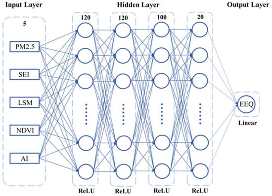
Figure 3. Structure of the DNN model.

2.2.3. Dynamic Trend Analysis of EEQ

The Sen and Mann–Kendall (MK) tests were used to analyze the dynamic trend of EEQ. The Sen test evaluates the slope of a time series to determine whether the trend is increasing or decreasing. It was used to assess whether the EEQ time series had a monotonic upward or downward trend. The Sen test uses a linear model to estimate the slope of the trend. The trend β is calculated as follows [38]:

$$\mathsf{\beta }=Median{({\displaystyle \frac{x_j-x_i}{j-i}})}^2,2013\le i\le 2020$$

(6)

where x_j and x_i are the EEQ values in the i-th and j-th years, respectively, and Median is the median function. β represents the variation trend; β > 0 indicates an increasing trend, and β < 0 represents a decreasing trend.

The MK test is a nonparametric method to evaluate whether a trend in time-series data is statistically significant. When n < 10, the MK test uses statistic S, which is calculated as follows [39]:

$$\mathrm{S}={\displaystyle \sum _{i=1}^{n-1}{\displaystyle \sum _{j=i+1}^n\mathrm{sgn}(x_j-x_i)}}$$

(7)

$$\mathrm{sgn}(x_i-x_j)=\left\{\begin{array}{r}1\left(x_j-x_i>0\right)\\ 0\left(x_j-x_i=0\right)\\ -1\left(x_j-x_i<0\right)\end{array}\right.$$

(8)

where n (=8) is the length of the time series, and i and j range from 2013 to 2020. If |S| ≥ Sα/2 (Sα/2 = 14), the null hypothesis is rejected, indicating that the time-series EEQ data have a significant trend [40].

The judgment criteria for determining the type and significance of the EEQ trend are listed in Table 6.

Table 6. The judgment criterion for determining the type and significance of the EEQ trend.

Judgment Criterion	Dynamic EEQ Trend
β > 0 and |S| > 14	Significant increase
β > 0 and |S| ≤ 14	Non-significant increase
β < 0 and |S| ≤ 14	Non-significant decrease
β < 0 and |S| > 14	Significant decrease

2.2.4. Accuracy Evaluation

The determination coefficient (R²) and the normalized root mean square error (NRMSE) were selected to evaluate the performance of the EEQ evaluation model and the accuracy of the ecological indices. A larger R² value and smaller NRMSE value indicate a higher accuracy of the prediction model and indices. The expressions are expressed as follows [41,42]:

$$R^2=1-{\displaystyle \frac{{\displaystyle {\sum }_{i=1}^n(y_i-{\stackrel{⌢}{y}}_i{)}^2}}{{\displaystyle {\sum }_{i=1}^n(y_i-{\overline{y}}_i{)}^2}}}$$

(9)

$$\mathrm{NRMSE}={\displaystyle \frac{\sqrt{\frac{1}{\mathrm{n}}{\displaystyle {\sum }_{\mathrm{i}=1}^{\mathrm{n}}({\mathrm{y}}_{\mathrm{i}}-{\stackrel{⌢}{\mathrm{y}}}_{\mathrm{i}}{)}^2}}}{\overline{\mathrm{y}}}}$$

(10)

where ${\mathrm{y}}_{\mathrm{i}}$ is the measured value of the ith sample, $\widehat{{\mathrm{y}}_{\mathrm{i}}}$ is the estimated value of the ith sample, $\overline{\mathrm{y}}$ is the average value of the measured values, and n is the number of samples.

3. Results

3.1. RSIs in the PSR Framework

The five RSIs (PM2.5, SEI, NDVI, LSM and AI) in the PSR framework were generated based on Equations (1)–(3) and the multi-source time-series imagery data. The spatial distributions of these RSIs in Guangzhou are presented in Figure 4.

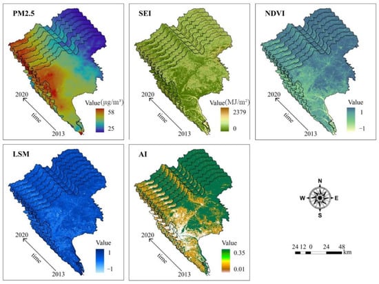
Figure 4. Spatial distribution of the RSIs in Guangdong province from 2013 to 2020.

Pearson correlation analysis was performed between the five RSIs and the EEQ to test the impact of each indicator on the EEQ task. Figure 5 shows the correlation coefficients (r). Significant positive correlations occurred between EEQ and NDVI (r of 0.88), AI (r of 0.88), and LSM (r of 0.76), whereas EEQ was significantly and negatively correlated with SEI (r of −0.87) and PM2.5 (r of −0.52). The correlations of these two sets of variables had opposite signs, indicating that they had opposite effects on EEQ, consistent with actual conditions. The result validated that EEQ had a high correlation with five RSIs (p < 0.01), indicating that the five indicators were appropriate for evaluating EEQ.

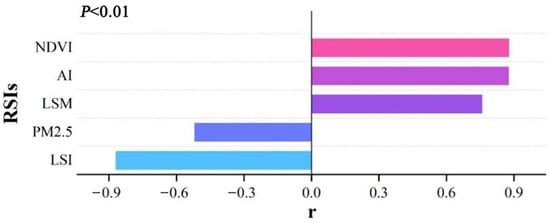
Figure 5. Correlation between EEQ and the five RSIs.

3.2. Performance of the DNN for Evaluating EEQ

The EEQ evaluation model was developed using the DNN algorithm based on 260 training samples (blue plots in Figure 1). In this study, the parameters of the model were determined based on existing studies and numerous experiments [36]. The initial learning rate was set to 0.001, the epoch was 200, the batch size was 16, and the number of hidden layers was four with the neuron structure of 120-120-100-20. The dropout rate was set to 0.4. Figure 6a presents the modeling accuracy of the model with an R² of 0.84 and an NRMSE of 8.85%, indicating that the DNN evaluation model has a high predictive accuracy for evaluating EEQ. In addition, we used 113 test samples (pink plots in Figure 1) to validate the estimation accuracy of the DNN model, shown in Figure 6b. The R² is 0.81, and the NRMSE is 10.90%; the majority of the points are close to the 1:1 line, indicating the reliability of the model.

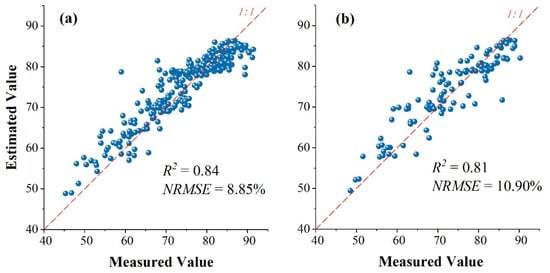
Figure 6. Scatterplots of measured versus estimated values of EEQ based on (a) 260 training samples and (b) 113 testing samples.

3.3. Spatial Distribution and Dynamic Changes in EEQ in the Guangzhou Study Area

3.3.1. Spatial Distribution of EEQ

The constructed DNN model was used to map EEQ in Guangzhou from 2013 to 2020 (Figure 7). The spatial distribution of EEQ in Guangzhou is heterogeneous, with an increasing trend from southwest to northeast. Regions with lower EEQ are located in the southern and central western downtown areas close to the sea, with relatively low elevations and frequent human activities [43]. Areas with higher EEQ occur in the northeastern mountainous region, which has relatively high elevation, high forest cover, and low urbanization, consistent with actual conditions.

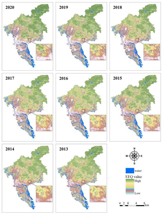
Figure 7. Spatial distribution of EEQ in Guangzhou from 2013 to 2020.

Moreover, 34 measured EEQ values in Guangzhou were used to validate the mapping accuracy of the DNN model (Figure 8). The result shows that the DNN provides good performance for estimating EEQ at the regional scale, with an R² of 0.75 and an NRMSE of 13.61%.

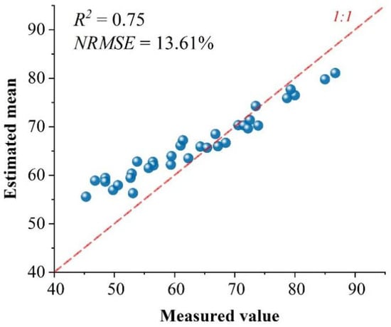
Figure 8. Scatterplots of measured values versus estimated values of EEQ based on 34 validation samples.

3.3.2. Dynamic Changes in EEQ

Statistical methods were used to analyze the EEQ trend. Figure 9a shows the boxplot of the EEQ values in Guangzhou from 2013 to 2019, indicating significant interannual fluctuations in the EEQs. The TCESE 2015 was used to classify the EEQ levels, and the percentage of area in different levels was calculated as shown in Figure 9b. There is an overall increase in the median, mean, upper quartile, and range of the EEQ values, whereas the lower quartile decreased overall. The proportion of excellent and moderate EEQ levels increased from 2013 to 2019, whereas the proportion of the good EEQ level decreased. The proportion of the excellent level increased more than that of the moderate level, accounting for the largest proportion ultimately. The results show that the EEQ of Guangzhou improved during the study period due to environmental protection policies (http://sthjj.gz.gov.cn/ (accessed on 11 December 2025)), although localized environmental degradation occurred as a result of urbanization.

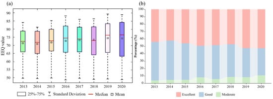
Figure 9. Statistical results of (a) boxplot of the EEQ values and (b) area distribution of EEQ levels in Guangzhou from 2013 to 2019.

Figure 10 shows the classification results of the EEQ trends in Guangzhou based on the Sen and MK tests. For β > 0 and |S| > 14, the EEQ increased significantly. These areas accounted for 49.61% of the total area of Guangzhou. Regions with a significant increase in EEQ occurred mainly in the northeast of Guangzhou. Areas with a non-significant increase in EEQ (β > 0 and |S| ≤ 14) accounted for 19.22% of the total area. Regions with a non-significant decrease in EEQ (β < 0 and |S| ≤ 14) comprised 15.5% of the total area, and areas with a significant decrease in EEQ (β < 0 and |S| > 14) accounted for 16.67% of the total area. Regions with a significant decrease in EEQ were located in the western, central, and southern parts of Guangzhou. The results of the dynamic trend analysis show that areas with a good EEQ level are getting better, whereas areas with worse EEQ levels are getting poorer. The former areas are primarily located within ecological protection zones implemented by the government, such as ecological protection red-line areas. Areas with a significant decline in EEQ are located in built-up regions of rapid urbanization, accompanied by continuous development and large-scale expansion of urban areas.

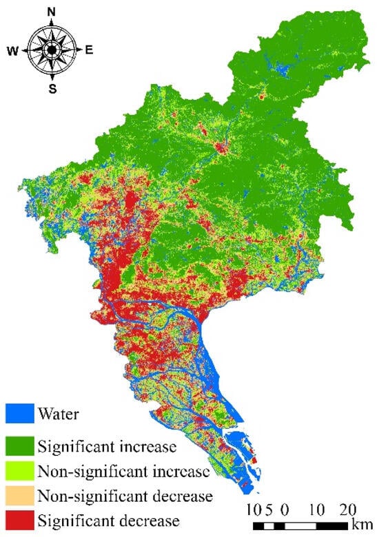
Figure 10. Classification results of the EEQ trends based on the Sen and Mann–Kendall tests in Guangzhou from 2013 to 2020.

4. Discussion

4.1. Comparison with Similar Studies

Previous EEQ evaluation methods provided valuable information but had limitations. First, studies using RS evaluation methods primarily used single indicators (such as NDVI) to evaluate EEQ [44]. Although this method is straightforward due to the accessibility of the single vegetation indicator, it cannot accurately assess EEQ due to the lack of consideration of other environmental factors (e.g., water network density, pollution load, and land stress). Some studies used multiple indicators to evaluate EEQ, improving the accuracy over a single indicator; however, these RS indicators were not combined with traditional indicators to quantify EEQ, excluding pressure indicators (e.g., the Pollution Load Index, PLI), resulting in inadequate evaluation of human activity impacts. Furthermore, the weight allocation via principal component analysis (PCA) may deviate from ecological significance. We chose the RSIs of the PSR framework (Table 2) after evaluating the data and conducting a literature review and extensive experiments to ensure that the indicators corresponded to traditional indicators.

Second, previous studies described the relationship between RSIs and EEQ or replaced EEQ values with RSEIs [45]. However, they did not establish a relationship model between EEQ and RSIs to directly quantify EEQ; thus, these studies lack quantitative information on EEQ and cannot be verified by ground truth data. In this study, the DNN algorithm was used to model the nonlinear relationship between EEQ and five RSIs (PM_2.5, SEI, NDVI, LSM, and AI). Unlike traditional linear-weighted or PCA-based methods that assume linearity or orthogonality among indicators, DNN can capture complex nonlinear interactions and higher-order dependencies among ecological variables, which are common in real environmental systems. As a result, the quantitative model achieved high accuracy at both the sample-point scale (R² = 0.81) and the regional scale (R² = 0.75), demonstrating the theoretical and practical advantages of DNN for EEQ estimation.

Third, this study focused on using RSIs in the PSR framework to quantify EEQ. We compared the proposed approach with the commonly used RSEI method to verify the accuracy and reliability of our approach for practical applications. We calculated RSEI in Guangzhou in 2013, 2016, and 2019. As shown in Figure 11, the EEQ spatial distributions obtained from the RSEI method and the proposed method are similar. However, the EEQ values are lower for the RSEI method than for the proposed method. A total of 34 samples (pink plots in Figure 2) were utilized to validate the estimated accuracies of EEQ for both methods. Figure 12 shows that the proposed method has a higher R² (0.75) and a lower NRMSE (13.61%) than the RSEI method (R² of 0.51 and NRMSE of 19.13%), suggesting that the proposed method is more reliable for evaluating EEQ. This study quantified EEQ directly using remote sensing techniques for the first time, which improved the accuracy and general applicability of EEQ evaluation using traditional remote sensing techniques.

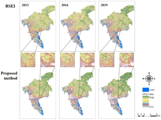
Figure 11. Comparison of EEQ in Guangzhou from 2013 to 2019 derived from the RSEI method and the proposed method.

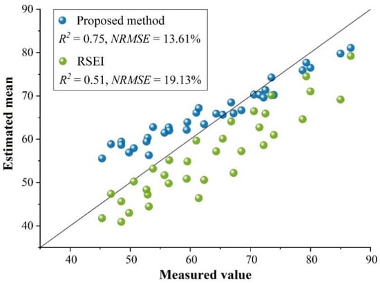
Figure 12. Measured and estimated EEQ values derived from the RSEI method and the DNN model.

Finally, the average EEQ values (Figure 9a) have increased significantly since 2013. The results of the EEQ trend analysis also demonstrate that areas with an increase in EEQ were larger than those with a decrease in EEQ in Guangzhou between 2013 and 2020. Areas with a significant increase in EEQ occurred mainly in the northeastern part of Guangzhou, and the regions with a significant decrease in EEQ were mainly concentrated in the western, central, and southern parts of Guangzhou. Overall, the classification results of the EEQ trends were consistent with the results of previous studies [35]. The findings showed that areas with a good EEQ level improved, and areas with a poor EEQ level degraded, which was attributed to policies aimed at protecting ecological reserves, such as the delineation of red-line areas. In non-reserve areas, urbanization and continuous development led to a deterioration in the EEQ in built-up areas.

4.2. Prospects for Future Studies

Owing to the limited EEQ sample data available for Guangzhou City specifically, the estimation model was developed using data from Guangdong Province. The study area was focused on Guangzhou to address urban ecological issues. Given the constraints of processing the extensive provincial time-series imagery, future work will aim to apply this method across the entire Guangdong Province. Moreover, the sample data used in this study to evaluate EEQ was at the county scale, resulting in low accuracy of the model’s estimates at fine scales; however, it enabled EEQ mapping at different scales. More fine-scale sample-point data will be collected in the future to improve the accuracy of the model evaluation.

The DNN algorithm requires a large sample size to construct a stable model, which limits its applicability in data-scarce regions. To overcome this challenge, some methods will be introduced as follows: (1) implementing transfer learning techniques by pre-training models on data-rich regions and fine-tuning them for target areas with limited samples; (2) exploring ensemble learning methods (e.g., Random Forest–DNN hybrid models) to improve model robustness with smaller datasets; and (3) incorporating data augmentation strategies to expand the effective training sample size.

In this study, there is still a shortage of RSIs in the PSR framework, and the combination of RSIs and traditional indicators must be improved. RSIs that are more sensitive to EEQ should be chosen. For instance, PLI or further research will incorporate more pollution factors to develop a remote sensing-based pollution load indicator, enabling rapid and accurate reflection of ecological pollution and enhancing the remote sensing evaluation system for estimating EEQ. In addition, the length of the time series should be increased to evaluate long-term trends in EEQ. We will address these limitations in our future work.

5. Conclusions

A new method was proposed to quantitatively evaluate EEQ using RSIs in the PSR framework. We chose RSIs based on the traditional EEQ evaluation system and established a DNN model to describe the relationship between EEQ and the RSIs. We conducted modeling and mapping validations in Guangdong province and Guangzhou, respectively. The results showed that the DNN model provided good performance for estimating EEQ with a modeling accuracy of R² = 0.84 and an NRMSE of 8.85%. The mapping accuracy of EEQ was also relatively high, with an R² of 0.75 and an NRMSE of 13.61%. The proposed method had a higher EEQ estimation accuracy than the RSEI method (R² of 0.51 and NRMSE of 19.13%). Moreover, the Sen and MK tests were used to analyze the EEQ trends in Guangzhou city from 2013 to 2020. The results showed that the proportion of areas with an increasing EEQ trend (49.61%) was greater than that with a decreasing trend (16.67%). Most of these areas were located in the northeast of Guangzhou and the western, central, and southern parts of Guangzhou, respectively, corresponding to actual conditions. Our results indicate that the proposed approach has substantial potential for the accurate estimation of EEQ at the regional scale. To the best of our knowledge, this is the first study to quantify EEQ using RSIs in the PSR framework.

References

- Tahiru, A.-W.; Cobbina, S.; Asare, W.; Takal, S.U. Advancing Environmental Sustainability through Remote Sensing: A Review of Applications, Limitations, and Emerging Solutions. Preprints 2025. [Google Scholar] [CrossRef]
- Gou, R.; Zhao, J. Eco-Environmental Quality Monitoring in Beijing, China, Using an RSEI-Based Approach Combined with Random Forest Algorithms. IEEE Access 2020, 8, 196657–196666. [Google Scholar] [CrossRef]
- Wang, H.; Liu, C.; Zang, F.; Liu, Y.; Chang, Y.; Huang, G.; Fu, G.; Zhao, C.; Liu, X. Remote Sensing-Based Approach for the Assessing of Ecological Environmental Quality Variations Using Google Earth Engine: A Case Study in the Qilian Mountains, Northwest China. Remote Sens. 2023, 15, 960. [Google Scholar] [CrossRef]
- Karimian, H.; Zou, W.; Chen, Y.; Xia, J.; Wang, Z. Landscape Ecological Risk Assessment and Driving Factor Analysis in Dongjiang River Watershed. Chemosphere 2022, 307, 135835. [Google Scholar] [CrossRef] [PubMed]
- Boori, M.S.; Choudhary, K.; Paringer, R.; Kupriyanov, A. Eco-Environmental Quality Assessment Based on Pressure-State-Response Framework by Remote Sensing and GIS. Remote Sens. Appl. Soc. Environ. 2021, 23, 100530. [Google Scholar] [CrossRef]
- Wu, S.; Gao, X.; Lei, J.; Zhou, N.; Guo, Z.; Shang, B. Ecological Environment Quality Evaluation of the Sahel Region in Africa Based on Remote Sensing Ecological Index. J. Arid Land 2022, 14, 14–33. [Google Scholar] [CrossRef]
- Maity, S.; Das, S.; Pattanayak, J.M.; Bera, B.; Shit, P.K. Assessment of Ecological Environment Quality in Kolkata Urban Agglomeration, India. Urban Ecosyst. 2022, 25, 1137–1154. [Google Scholar] [CrossRef]
- Roy, S.; Bose, A.; Majumder, S.; Roy Chowdhury, I.; Abdo, H.G.; Almohamad, H.; Abdullah Al Dughairi, A. Evaluating Urban Environment Quality (UEQ) for Class-I Indian City: An Integrated RS-GIS Based Exploratory Spatial Analysis. Geocarto Int. 2022, 38, 2153932. [Google Scholar] [CrossRef]
- Lv, J.; Zhou, W. Ecological Environmental Quality in China: Spatial and Temporal Characteristics, Regional Differences, and Internal Transmission Mechanisms. Sustainability 2023, 15, 3716. [Google Scholar] [CrossRef]
- Cai, Z.; Zhang, Z.; Zhao, F.; Guo, X.; Zhao, J.; Xu, Y.; Liu, X. Assessment of Eco-Environmental Quality Changes and Spatial Heterogeneity in the Yellow River Delta Based on the Remote Sensing Ecological Index and Geo-Detector Model. Ecol. Inform. 2023, 77, 102203. [Google Scholar] [CrossRef]
- Wei, J.; Li, Z.; Lyapustin, A.; Sun, L.; Peng, Y.; Xue, W.; Su, T.; Cribb, M. Reconstructing 1-Km-Resolution High-Quality PM2.5 Data Records from 2000 to 2018 in China: Spatiotemporal Variations and Policy Implications. Remote Sens. Environ. 2021, 252, 112136. [Google Scholar] [CrossRef]
- Wei, Z.; Peijun, D.; Shanchuan, G.; Cong, L.; Hongrui, Z.; Pingjie, F. Enhanced Remote Sensing Ecological Index and Ecological Environment Evaluation in Arid Area. Natl. Remote Sens. Bull. 2023, 27, 299–317. [Google Scholar]
- Liu, Y.; Xiang, W.; Hu, P.; Gao, P.; Zhang, A. Evaluation of Ecological Environment Quality Using an Improved Remote Sensing Ecological Index Model. Remote Sens. 2024, 16, 3485. [Google Scholar] [CrossRef]
- Foga, S.; Scaramuzza, P.L.; Guo, S.; Zhu, Z.; Dilley, R.D., Jr.; Beckmann, T.; Schmidt, G.L.; Dwyer, J.L.; Hughes, M.J.; Laue, B. Cloud Detection Algorithm Comparison and Validation for Operational Landsat Data Products. Remote Sens. Environ. 2017, 194, 379–390. [Google Scholar] [CrossRef]
- Wang, Y.; Ding, Q.; Zhuang, D. An Eco-City Evaluation Method Based on Spatial Analysis Technology: A Case Study of Jiangsu Province, China. Ecol. Indic. 2015, 58, 37–46. [Google Scholar] [CrossRef]
- Zhu, M.; Liu, S.; Xia, Z.; Wang, G.; Hu, Y.; Liu, Z. Crop Growth Stage GPP-Driven Spectral Model for Evaluation of Cultivated Land Quality Using GA-BPNN. Agriculture 2020, 10, 318. [Google Scholar] [CrossRef]
- Adriaanse, A. Environmental Policy Performance Indicators; Ministerie van Volkshuisvesting, Ruimtelijke Ordening en Milieubeheer: The Hague, The Netherlands, 1993. [Google Scholar]
- Xu, H.; Wang, M.; Shi, T.; Guan, H.; Fang, C.; Lin, Z. Prediction of Ecological Effects of Potential Population and Impervious Surface Increases Using a Remote Sensing Based Ecological Index (RSEI). Ecol. Indic. 2018, 93, 730–740. [Google Scholar] [CrossRef]
- Zhao, G.; Chen, L.; Mu, J. Discussion on Construction of Ecological Environment Quality Evaluation System. Meteorol. Environ. Sci 2018, 41, 1–11. [Google Scholar]
- Yue, H.; Liu, Y.; Li, Y.; Lu, Y. Eco-Environmental Quality Assessment in China’s 35 Major Cities Based on Remote Sensing Ecological Index. IEEE Access 2019, 7, 51295–51311. [Google Scholar] [CrossRef]
- Ali, M.B.; Jamal, S. Modelling the Present and Future Scenario of Urban Green Space Vulnerability Using PSR Based AHP and MLP Models in a Metropolitan City Kolkata Municipal Corporation. Geol. Ecol. Landsc. 2025, 9, 1141–1159. [Google Scholar] [CrossRef]
- Sun, Y.; Zeng, Q.; Geng, B.; Lin, X.; Sude, B.; Chen, L. Deep Learning Architecture for Estimating Hourly Ground-Level PM 2.5 Using Satellite Remote Sensing. IEEE Geosci. Remote Sens. Lett. 2019, 16, 1343–1347. [Google Scholar] [CrossRef]
- Shao, J.; Huang, K.; Tang, W.; Liang, X.; Wu, W.; Huang, G. Discussion on the Construction of Ecological Water Network in Guangxi Province of China. Res. Ecol. 2021, 3, 8–13. [Google Scholar] [CrossRef]
- Peri, P.; Lasagno, R.; Chartier, M.; Roig, F.; Rosas, Y.; Pastur, G. Soil Erosion Rates and Nutrient Loss in Rangelands of Southern Patagonia; Elsevier: Amsterdam, The Netherlands, 2022; pp. 102–110. [Google Scholar]
- Shan, W.; Jin, X.; Ren, J.; Wang, Y.; Xu, Z.; Fan, Y.; Gu, Z.; Hong, C.; Lin, J.; Zhou, Y. Ecological Environment Quality Assessment Based on Remote Sensing Data for Land Consolidation. J. Clean. Prod. 2019, 239, 118126. [Google Scholar] [CrossRef]
- Xu, D.; Yang, F.; Yu, L.; Zhou, Y.; Li, H.; Ma, J.; Huang, J.; Wei, J.; Xu, Y.; Zhang, C.; et al. Quantization of the Coupling Mechanism between Eco-Environmental Quality and Urbanization from Multisource Remote Sensing Data. J. Clean. Prod. 2021, 321, 128948. [Google Scholar] [CrossRef]
- Chen, T.; Niu, R.; Li, P.; Zhang, L.; Du, B. Regional Soil Erosion Risk Mapping Using RUSLE, GIS, and Remote Sensing: A Case Study in Miyun Watershed, North China. Environ. Earth Sci. 2011, 63, 533–541. [Google Scholar] [CrossRef]
- Williams, J.; Renard, K.; Dyke, P. EPIC: A New Method for Assessing Erosion’s Effect on Soil Productivity. J. Soil Water Conserv. 1983, 38, 381–383. [Google Scholar] [CrossRef]
- Coulibaly, L.K.; Guan, Q.; Assoma, T.V.; Fan, X.; Coulibaly, N. Coupling Linear Spectral Unmixing and RUSLE2 to Model Soil Erosion in the Boubo Coastal Watershed, Côte d’ivoire. Ecol. Indic. 2021, 130, 108092. [Google Scholar] [CrossRef]
- Kefi, M.; Yoshino, K.; Setiawan, Y. Assessment and Mapping of Soil Erosion Risk by Water in Tunisia Using Time Series MODIS Data. Paddy Water Environ. 2012, 10, 59–73. [Google Scholar] [CrossRef]
- Fu, S.; Liu, B.; Zhou, G.; Sun, Z.; Zhu, X. Calculation Tool of Topographic Factors. Sci. Soil Water Conserv. 2015, 13, 105–110. [Google Scholar]
- Van der Knijff, J.; Jones, R.; Montanarella, L. Soil Erosion Risk Assessment in Europe; European Soil Bureau: Ispra, Italy, 2000. [Google Scholar]
- Fang, G.; Yuan, T.; Zhang, Y.; Wen, X.; Lin, R. Integrated Study on Soil Erosion Using RUSLE and GIS in Yangtze River Basin of Jiangsu Province (China). Arab. J. Geosci. 2019, 12, 173. [Google Scholar] [CrossRef]
- Zhu, L.; Li, D.; Wei, X.; Zhang, H. The Current Situation of Soil Erodibility (K) Value and Its Impact Factors in Guangdong Province. Subtrop. Soil Water Conserv. 2007, 19, 4–7. [Google Scholar]
- Yuan, Q.; Shen, H.; Li, T.; Li, Z.; Li, S.; Jiang, Y.; Xu, H.; Tan, W.; Yang, Q.; Wang, J.; et al. Deep Learning in Environmental Remote Sensing: Achievements and Challenges. Remote Sens. Environ. 2020, 241, 111716. [Google Scholar] [CrossRef]
- Chuan, C.; Zheng, C.; Bo, L.; Ligang, L. Computation of Atmospheric Optical Parameters Based on Deep Neural Network and PCA. IEEE Access 2020, 8, 102256–102262. [Google Scholar] [CrossRef]
- He, Q.; Wang, Z.; Li, J. Application of the Deep Neural Network in Retrieving the Atmospheric Temperature and Humidity Profiles from the Microwave Humidity and Temperature Sounder Onboard the Feng-Yun-3 Satellite. Sensors 2021, 21, 4673. [Google Scholar] [CrossRef] [PubMed]
- Jiang, W.; Yuan, L.; Wang, W.; Cao, R.; Zhang, Y.; Shen, W. Spatio-Temporal Analysis of Vegetation Variation in the Yellow River Basin. Ecol. Indic. 2015, 51, 117–126. [Google Scholar] [CrossRef]
- Xu, H.; Wang, Y.; Guan, H.; Shi, T.; Hu, X. Detecting Ecological Changes with a Remote Sensing Based Ecological Index (RSEI) Produced Time Series and Change Vector Analysis. Remote Sens. 2019, 11, 2345. [Google Scholar] [CrossRef]
- Gilbert, R.O. Statistical Methods for Environmental Pollution Monitoring; John Wiley & Sons: Hoboken, NJ, USA, 1987. [Google Scholar]
- Chen, S.; Xu, H.; Xu, D.; Ji, W.; Li, S.; Yang, M.; Hu, B.; Zhou, Y.; Wang, N.; Arrouays, D.; et al. Evaluating Validation Strategies on the Performance of Soil Property Prediction from Regional to Continental Spectral Data. Geoderma 2021, 400, 115159. [Google Scholar] [CrossRef]
- Ran, H.; Kang, S.; Li, F.; Du, T.; Tong, L.; Li, S.; Ding, R.; Zhang, X. Parameterization of the AquaCrop Model for Full and Deficit Irrigated Maize for Seed Production in Arid Northwest China. Agric. Water Manag. 2018, 203, 438–450. [Google Scholar] [CrossRef]
- Xiong, Y.; Xu, W.; Lu, N.; Huang, S.; Wu, C.; Wang, L.; Dai, F.; Kou, W. Assessment of Spatial–Temporal Changes of Ecological Environment Quality Based on RSEI and GEE: A Case Study in Erhai Lake Basin, Yunnan Province, China. Ecol. Indic. 2021, 125, 107518. [Google Scholar] [CrossRef]
- Furberg, D.; Ban, Y.; Nascetti, A. Monitoring of Urbanization and Analysis of Environmental Impact in Stockholm with Sentinel-2A and SPOT-5 Multispectral Data. Remote Sens. 2019, 11, 2408. [Google Scholar] [CrossRef]
- Hu, X.; Xu, H. A New Remote Sensing Index for Assessing the Spatial Heterogeneity in Urban Ecological Quality: A Case from Fuzhou City, China. Ecol. Indic. 2018, 89, 11–21. [Google Scholar] [CrossRef]
Disclaimer/Publisher’s Note: The statements, opinions and data contained in all publications are solely those of the individual author(s) and contributor(s) and not of MDPI and/or the editor(s). MDPI and/or the editor(s) disclaim responsibility for any injury to people or property resulting from any ideas, methods, instructions or products referred to in the content. |
© 2025 by the authors. Licensee MDPI, Basel, Switzerland. This article is an open access article distributed under the terms and conditions of the Creative Commons Attribution (CC BY) license.