Assessing the Performance of Multiple Satellite-Based Evapotranspiration Models over Tropical Forests

Highlights

What are the main findings?

• The four remote sensing-based evapotranspiration models (SSEBop, geeSEBAL, PT-JPL and T-SEB) showed good agreement with in situ flux tower data over global tropical forests.
• Models’ performance varied regionally and depended on the meteorological forcing used.

What are the implications of the main findings?

• This study demonstrates that current high-resolution remote sensing models are effective and viable tools for monitoring evapotranspiration in complex tropical forests, helping to overcome challenges like data scarcity.
• These models are particularly valuable for quantifying the hydrological impacts of deforestation and climate change.

Abstract

Tropical forests are critical regulators of global water and energy cycles, with evapotranspiration ($ET$) being a key ecohydrological process. However, monitoring $ET$ over tropical forests is a challenge due to their complex structure, and the logistical difficulties in obtaining observations that are both spatially representative and have wide coverage. Remote sensing data offer an alternative to these limitations, although the effectiveness of $ET$ remote sensing-based models over these areas is not well-known. Thus, this study evaluates the performance of four remote sensing-based $ET$ models (SSEBop, geeSEBAL, PT-JPL and T-SEB) in tropical forests. We compared models’ estimations against flux tower observations and assessed the uncertainty in models’ outputs driven by different meteorological input forcings. Additionally, we conducted a spatial–temporal analysis of models’ response to the impact of deforestation on $ET$ patterns. Our results showed a good agreement between modeled and observed $ET$ using the most accurate meteorological input dataset (RMSEs ranging from 1.1 to 1.3 mm.day⁻¹ for ERA5-Land). The deforestation analysis for sites in Africa, America and Asia revealed an agreement of the models in demonstrating the impact of deforestation on $ET$, though performance varied due to different deforestation patterns. For the long-term results, models showed different responses to forest removal, highlighting the uncertainties of the individual models and underscoring the necessity of multi-model approaches in providing more accurate information. These findings demonstrate that current high-resolution remote sensing models can effectively monitor $ET$ in tropical forests on a global scale, especially for assessing the impacts of deforestation in data-scarce regions.

1. Introduction

Tropical forests are fundamental for regulating Earth’s hydrological and energy cycles through the process of evapotranspiration ($ET$) by transporting large volumes of water vapor into the atmosphere [1,2]. This process regulates energy transfer, cooling the surface, modulating regional climate and rainfall patterns [3,4,5]. Despite comprising just 7% of the Earth’s land surface [6], tropical forests generate nearly 33% of terrestrial $ET$ [7]. In terms of precipitation recycling, around 50% of the Amazon’s tropical forest precipitation is a consequence of local $ET$ [8], while 24% to 39% of $ET$ from the Congo tropical forest is recycled as local rainfall [3,9].

Anthropogenic influences have induced changes in spatial–temporal patterns of $ET$ over the last decades. Global warming is known to exacerbate heat stress [10,11], which in turn intensifies the frequency and severity of major disturbances, degrading ecosystem resilience [12,13]. While climate change alters the function of primary forests, deforestation impacts the global climate through the removal of forests for activities such as agriculture, cattle ranching and mining [14,15,16,17]. For instance, forest loss in Asia has been shown to alter monsoon circulation and precipitation [18,19], while numerous studies link deforestation in the Amazon to shifting regional rainfall patterns [20,21,22,23]. These changes are linked to a reduction in $ET$ [4,17,24,25], increasing the vulnerability of these ecosystems [26]. Studies suggest that if current loss rates persist, tropical forests in the Amazon could overpass a critical threshold, triggering significant shifts in global climate circulation [27,28], interrupting precipitation recycling [4,5], and potentially pushing tropical areas into drier conditions [29,30].

Understanding the hydroclimate consequences of tropical deforestation and climate change remains a challenge. Deforestation occurs in complex, fragmented patches, yet most analyses rely on global climate models whose coarse spatial resolution cannot accurately capture these fine-scale impacts on $ET$ [2,17,31,32,33], highlighting the need for high-resolution approaches to monitor water cycling. Moreover, while eddy covariance (EC) in situ observations have significantly improved our understanding of deforestation consequences [34,35], the low density of the networks over tropical areas and logistical difficulties limit their application. Thus, remote sensing offers a powerful tool to overcome both the coarse resolution of these models and the scarcity of in situ observations. Remote sensing-based $ET$ models are widely used for $ET$ monitoring [36,37,38,39,40], particularly in agriculture for efficient water use management [41]. State-of-the-art models estimate $ET$ by applying principles of surface energy conservation and aerodynamic heat, using satellite-delivered proxies like land surface temperature ($T_{rad})$ and vegetation indices (e.g., $NDVI$). However, most of these models were originally developed for agriculture applications [42,43], with empirical parameters often calibrated for the specific structure and phenology of crops. Therefore, their performance and uncertainty over complex areas such as tropical forests are not yet well understood, highlighting a critical need for further investigation.

The main goal of this study is to evaluate the capabilities and limitations of high-resolution, remote sensing-based $ET$ models for monitoring tropical forests. Specifically, we aim to (1) assess the performance of four distinct models (SSEBop, geeSEBAL, PT-JPL and T-SEB) by comparing their estimates against in situ data from a global network of flux towers; (2) quantify model uncertainty through a sensitivity analysis of meteorological inputs; and (3) evaluate the capability of each model to capture $ET$ changes due to deforestation.

2. Materials and Methods

2.1. Flux Towers Sites

We evaluated models’ accuracy by comparing $ET$ estimates against in situ observations from EC flux towers located in natural tropical forests (between 23° S and 23° N). These towers obtain observations of sensible ($H$) and latent heat flux ($LE$), which are used to estimate daily $ET$. A common issue with EC data is the lack of energy balance closure [44]. Therefore, we corrected the fluxes by partitioning the residual energy based on the Bowen ratio method [45]. The complete post-processing and quality control algorithm applied to the flux data is publicly available on GitHub (https://github.com/Open-ET/flux-data-qaqc, version 0.2.2, accessed on 10 July 2025).

A total of 14 sites from the AmeriFlux (https://ameriflux.lbl.gov/, accessed on 28 October 2025) and FLUXNET (https://fluxnet.org/, accessed on 28 October 2025) networks were used for this validation. Figure 1 shows the geographical locations of these sites, while Table 1 provides more detailed characteristics. Five towers are located in Brazil, two in Peru and one tower in each of the following countries: Congo Republic, China, Costa Rica, French Guiana, Ghana, Malaysia and Zimbabwe.

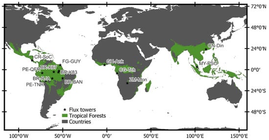
Figure 1. Geographic distribution of the 14 eddy covariance (EC) flux tower sites used in this study. Black stars show the sites’ location, and the green shaded area indicates the global extent of the tropical forests (based on Ecoregions dataset [46]).

Table 1. Description of the 14 flux towers used in this study.

Site	Country	Start Date	End Date	Lon.	Lat.	Reference
BR-BAN	Brazil	1 October 2003	1 December 2006	−50.161	−9.824	Borma et al. [47]
BR-K34	Brazil	6 January 1999	1 October 2006	−60.209	−2.609	Araújo et al. [48]
BR-K67	Brazil	1 January 2002	1 January 2012	−54.958	−2.856	Saleska et al. [49]
BR-K83	Brazil	1 January 2000	1 March 2004	−54.970	−3.017	da Rocha et al. [50]
BR-RJA	Brazil	23 March 1999	31 December 2002	−61.933	−10.078	Von Randow et al. [51]
CG-Tch	Congo Republic	1 February 2006	1 February 2010	11.656	−4.289	Merbold et al. [52]
CN-Din	China	1 February 2003	1 February 2006	112.536	23.173	Yu et al. [53]
CR-SoC	Costa Rica	1 January 2014	31 December 2014	−84.621	10.3827	Aparecido et al. [54]
FG-GUY	French Guiana	1 January 2004	31 December 2014	−52.924	5.278	Bonal et al. [55]
GH-Ank	Ghana	1 February 2011	1 February 2015	−2.694	5.268	Chiti et al. [56]
MY-PSO	Malaysia	1 February 2003	1 February 2010	102.306	2.973	Kosugi et al. [57]
PE-QFR	Peru	1 January 2018	31 December 2019	−73.318	−3.834	Griffis et al. [58]
PE-TNR	Peru	1 April 2019	31 December 2024	−69.283	−12.831	Vihermaa et al. [59]
ZM-Mon	Zimbabwe	1 August 2000	1 February 2010	23.252	−15.439	Merbold et al. [52]

2.2. Landsat Data

This study used Landsat Collection 2 Level-2 data to provide the necessary multispectral and thermal inputs for the $ET$ models. The dataset combines imagery from Landsat 5 (TM), Landsat 7 (ETM+), Landsat 8 (OLI/TIRS) and Landsat 9 (OLI-2/TIRS-2), all provided at 30 m spatial resolution with a 16-day revisit time. To mitigate the impact of cloud contamination [60], we only used images with less than 50% cloud cover. Remaining clouds and cloud shadows were then masked out using the accompanying quality assessment (QA) band.

2.3. Evapotranspiration Models

We evaluated the accuracy of four state-of-the-art, remote sensing-based $ET$ models. While all the $ET$ models are widely used globally, they differ significantly in their assumptions and parameterization schemes.

The SSEBop model [61,62,63] advantage is that it avoids the complex parameterization common to other energy balance $ET$ models. The model assumes that the evaporative fraction (${ET}_f$) can be calculated for each pixel by linearly scaling its surface temperature between hot (dry bulb) and cold (wet bulb) reference conditions through a psychrometric approach (Equation (1)). This process allows daily $ET$ to be estimated by multiplying the ${ET}_f$ by the alfafa reference $ET$ (${ET}_r$). For this study, we used the SSEBop version that employs the Forcing and Normalizing Operation (FANO) approach to estimate the cold surface temperature ($T_{cold}$; K units), which is delivered from air temperature [63].

$${ET}_f=1-{\gamma }^2\ast (T_{rad}-T_{cold}),$$

(1)

where $\gamma$ is the surface psychrometric constant [kPa.°C⁻¹] based on a dry condition surface.

A detailed derivation of the SSEBop equations is provided by Senay et al. [61,62,63].

The Priestley Taylor Jet Propulsor Laboratory (PT-JPL) [64] model is a process-based model that estimates daily $ET$ by partitioning it into canopy transpiration ($E_c^{ptjpl}$), soil evaporation ($E_s^{ptjpl}$) and interception loss ($E_i^{ptjpl}$). The total daily $ET$ is the sum of these terms. The model uses the Priestley–Taylor equation [65] to establish a potential $ET$ rate, which is then converted to actual daily $ET$ by applying biophysical constraints derived from satellite and meteorological data. The formula for canopy transpiration ($E_c^{ptjpl}$) can be calculated as follows (Equation (2)):

$$E_c^{ptjpl}=\left(1-f_{wet}\right)\ast f_g\ast f_T\ast f_{sm}\ast {\alpha }_{PT}\ast {\displaystyle \frac{∆}{∆+\gamma }}{R}_{nc},$$

(2)

where $f_{wet}$ is the fraction of the canopy surface that is wet, $f_g$ is the green canopy fraction, $f_T$ is the plant temperature constraint, $f_{sm}$ is the soil moisture constraint, ${\alpha }_{PT}$ is the Pristley–Taylor coefficient (1.26), $∆$ is the slope of the saturation vapor pressure–temperature curve [kPa.°C⁻¹], and $R_{nc}$ is the net radiation intercepted by the canopy [W.m⁻²].

The $E_s^{ptjpl}$ is calculated using Equation (3):

$$E_s^{ptjpl}= \left[f_{wet}+f_{sm} (1-f_{wet})\right]\ast {\alpha }_{PT}{\displaystyle \frac{∆}{∆+\gamma }}\left(R_{ns}-G\right),$$

(3)

where $R_{ns}$ is the radiation that reaches the soil [W.m⁻²] and $G$ is the instantaneous soil heat flux [W.m⁻²].

And the $E_i^{ptjpl}$ (Equation (4))

$$E_i^{ptjpl}=f_{wet}\ast {\alpha }_{PT}{\displaystyle \frac{∆}{∆+\gamma }}{R}_{nc},$$

(4)

A comprehensive description of the equations and formulation of PT-JPL is presented in Fisher et al. [64].

The Google Earth Engine Surface Energy Balance algorithm (geeSEBAL) model [66] solves each component of the energy balance equation, calculating the $LE$ as a residual. Instantaneous net radiation ($Rn$), soil heat ($G$) and $H$ fluxes can be estimate using Equations (5)–(7), respectively.

$$Rn=\left(1-\alpha \right){Rs}_{down }+{Rl}_{down }-{Rl}_{up }-\left(1-{\epsilon }_0\right) {Rs}_{down },$$

(5)

where ${Rs}_{down}$ and ${Rl}_{down}$ are the short- and longwave incident radiation [W.m⁻²], ${Rl}_{up}$ the outgoing long radiation [W.m⁻²], $\alpha$ the albedo and ${\epsilon }_0$ the surface emissivity.

$$G^{geesebal}=R_n(T_s-273.15)(0.0038+\left(0.0074 \alpha \right))(1-0.98 {\left(NDVI\right)}^4),$$

(6)

where $NDVI$ is the Normalized Difference Vegetation Index.

$$H={\displaystyle \frac{\rho cpdT}{r_{ah}}},$$

(7)

where $r_{ah}$ is the aerodynamic resistance [s.m⁻¹], $\rho$ is the atmospheric air density [kg.m⁻³] and $Cp$ is the specific heat of air at constant pressure [J.kg⁻¹.K⁻¹]. Since in Equation (7) $dT$ (the temperature difference between two heights above the surface) and $r_{ah}$ are unknown for every pixel, the equation is typically solved by assuming two extreme anchor pixels within the image, where the hot pixel represents a dry bare soil where all the energy available is converted in $H$ ($LE$ = 0), whereas the cold pixels represents a well-watered and full vegetated surface, which all the energy is converted into $LE$ ($H$ = 0).

By establishing a linear relationship between $T_{rad}$ and the $H$ using two anchor pixels, the model estimates $H$ for every pixel. The geeSEBAL model automates this anchor pixel selection based on the CIMEC algorithm [67], which identifies hot and cold conditions based on $NDVI$ and $T_{rad}$ percentiles within each scene.

Once the instantaneous $LE$ is determined ($LE = Rn - G - H$) the evaporative fraction is calculated ($EF = {\displaystyle \raisebox{1ex}{$LE$}\!\left/ \!\raisebox{-1ex}{$(Rn-G)$}\right.}$), and daily $ET$ is then computed under the assumption that the $EF$ is constant over a 24 h period (Equation (8)):

$${ET}^{geesebal}=0.0864 EF{\displaystyle \frac{R_{n 24h}}{ʎ}},$$

(8)

where $R_{n 24h}$ is the daily net radiation [W.m⁻²] and λ is the latent heat of vaporization [kJ kg⁻¹].

Further explanation of the equations underlying geeSEBAL is provided in Laipelt et al. [66].

The Two-Source Energy Balance (T-SEB) model [68] estimates daily $ET$ by partitioning energy fluxes between the soil and vegetation canopy. Unlike models that treat the land surface as a single flux, the T-SEB model acknowledges that soil evaporation $(E_s^{tseb})$ and canopy transpiration ${(E}_c^{tseb})$ are distinct processes driven by different temperatures and resistances. The model assumes that the $T_{rad}$ obtained by the satellite is a composite of the soil temperature ($T_s$) and the canopy temperature ($T_c$), which can be weighted by the fraction of vegetation cover ($f_c$), derived from the $NDVI$.

$$T_{rad}^{tseb}={(f_c\ast T_c^4+\left(1-f_c\right)\ast T_s^4)}^{0.25},$$

(9)

Norman et al. [68] developed a procedure to obtain daily $ET$ by using the Priestley–Taylor formulation to first estimate canopy latent heat flux (${LE}_c$), assuming that in the first step the vegetation is not stressed and well-watered (Equation (10)). Then, canopy sensible heat ($H_c$) can be estimate as a residual of the canopy balance energy equation ($H_c= R_{n c} - {LE}_c$), while Equation (11) is use to estimate $T_c$, and $T_s$ is estimated using Equation (9). Finally, ${LE}_s$ is calculated as a residual of the soil energy balance equation (${LE}_s = R_{ns} - G^{tseb} - H_s$), with $G^{tseb}$ and $H_s$ using Equation (12) and Equation (13), respectively.

$${LE}_c=\alpha {\displaystyle \frac{∆}{∆+\gamma }}{R}_{nc},$$

(10)

$$H_c=\rho cp{\displaystyle \frac{{(T}_c-T_{air})}{r_{ah}}}$$

(11)

$$G^{tseb}={0.35\ast R}_{ns}$$

(12)

$$H_s=\rho cp{\displaystyle \frac{{(T}_s-T_{air})}{r_{ah}}}$$

(13)

After this first step, if ${LE}_s$ is positive, then a solution for both ${LE}_s$ and ${LE}_c$ is obtained. On the other hand, if ${LE}_c$ is overestimated, this may lead to negative ${LE}_s$ values. As this condition is unlikely, an iterative process is performed by reducing the Priestley–Taylor coefficient ($\alpha$) each step (−0.1) until each pixel ${LE}_s$ is equal or above zero.

Finally, daily ${ET}^{tseb}$ is estimated by summing the contribution of $E_s^{tseb}$ and $E_c^{tseb}$ for each pixel.

Additional details on the equations used in T-SEB can be found in Norman et al. [68].

2.4. Evaluation of Meteorological Forcing Data

Since the $ET$ models depend on meteorological forcing data to represent atmospheric conditions and calculate reference $ET$ (${ET}_r$), we conducted a sensitivity analysis of the meteorological inputs for each model. The purpose of this analysis was to identify whether the models have low or high sensitivity to different meteorological forcings over tropical areas, given that reanalysis data are well known to have systematic biases in these regions [69,70]. We evaluated the models using widely used global meteorological datasets: ERA5-Land, CFSV2, GLDAS 2.1 and MERRA-2.

• ERA5-Land: produced by the European Centre for Medium-Range Weather Forecasts (ECMWF) [71], provides hourly data on 0.1° grid from 1950 to the present. It is an enhanced version of the ERA5 climate reanalysis, specifically designed for land surface applications.
• CFSV2 (Climate Forecast System Version 2): reanalysis dataset from the National Centers for Environmental Prediction (NCEP) [72], provides data at a 6-hourly frequency with a spatial resolution of 0.5°.
• GLDAS 2.1 (Global Land Data Assimilation System Version 2.1): jointly developed by NASA and NOAA agencies, provides land surface states and fluxes [73]. The 2.1 version provides data from 2000 to the present, with a 3-hourly temporal and 0.25° spatial resolution.
• MERRA-2 (Modern-Era Retrospective analysis for Research and Applications v2): produced by NASA’s Global Modeling and Assimilation Office (GMAO) [74], its data span from 1980 to the present at hourly scale, with a resolution of 0.5° latitude × 0.625° longitude.

The meteorological variables used by the models include the $T_{air}$ [K], the instantaneous downward shortwave radiation (${Sw}_{down})$ [W.m⁻²], and daily (${Sw}_{down}^{24h}$) [W.m⁻²], surface pressure ($P$) [Pa] and the wind speed ($ws$) [m.s⁻¹]. When not directly available, the relative humidity is computed ($RH={\displaystyle \raisebox{1ex}{$e_a$}\!\left/ \!\raisebox{-1ex}{$e_{sat}$}\right.}$) by calculating the saturated vapor pressure ($e_{sat}$) [kPa] from $T_{air}$ ($e=0.6108\mathrm{e}\mathrm{x}\mathrm{p}({\displaystyle \raisebox{1ex}{$17.27\ast T_{air}$}\!\left/ \!\raisebox{-1ex}{$237.3+T_{air}$}\right.})$). To calculate actual vapor pressure ($e_a$), we used dew point temperature ($T_{dew}$) in the previous equation in the absence of direct specific humidity ($q=0.622\ast ({\displaystyle \raisebox{1ex}{$e_a$}\!\left/ \!\raisebox{-1ex}{$P$}\right.})$) [kPa] data, as described by [75]. Table 2 shows the meteorological variables required by each model.

Table 2. Meteorological input variables required by each $ET$ model.

Model	Meteorological Inputs
SSEBop	$T_{air}$$, ws$ and ${Sw}_{down}^{24h}$
PT-JPL	$T_{air}$$, RH$$, {Sw}_{down}$$, P$ and $ws$
geeSEBAL	$T_{air}$$, RH$$, ws$$, {Sw}_{down}$ and ${Sw}_{down}^{24h}$
T-SEB	$T_{air},$$ws$ and ${Sw}_{down}$

2.5. Performance Evaluation

The performance of each model was evaluated using three statistical metrics: the root means square error ($RMSE$) (Equation (14)), the mean bias error ($BIAS$) (Equation (15)) and the $SLOPE$ (Equation (16)).

$$RMSE=\sqrt{{\displaystyle \frac{{\sum }_{i=1}^n{(E{T}_{obs}-{ET}_{model})}^2}{n}}},$$

(14)

$$BIAS={\displaystyle \frac{{\sum }_{i=1}^n({ET}_{obs}-{ET}_{model})}{n}},$$

(15)

$$\mathrm{S}\mathrm{L}\mathrm{O}\mathrm{P}\mathrm{E}={\displaystyle \frac{{\sum }_{i=1}^n{{ET}_{obs}}_i{{ET}_{model}}_i}{{\sum }_{i=1}^n{{ET}_{obs}}_i^2}},$$

(16)

where $n$ is the total number of daily ($i$) observations, ${ET}_{obs}$ is the $ET$ observed at the sites, and ${ET}_{model}$ is the $ET$ simulated by the model. Models’ average results were computed by considering a 3 × 3 pixel footprint centered on the flux tower coordinates.

3. Results

3.1. Performance of the ET Models

Overall, the results indicate a good agreement between the modeled and observed daily $ET$, considering the four remote sensing-based models and flux tower observations across global tropical forests (Figure 2). The ERA5-Land dataset was used as the meteorological forcing for this analysis due to its high accuracy (as discussed in Section 3.2). The SSEBop model yielded the highest accuracy, with an RMSE of 1.1 mm.day⁻¹, a $BIAS$ of 0.2 mm.day⁻¹ and a regression $SLOPE$ of 1.0. Following in performance was geeSEBAL, with an RMSE of 1.2 mm.day⁻¹ and a BIAS of 0.4 mm.day⁻¹ (SLOPE = 1.0). The PT-JPL and T-SEB models also performed well, with RMSE values of 1.2 mm.day⁻¹ and 1.3 mm.day⁻¹, respectively. Notably, T-SEB showed a slight tendency for underestimation, as indicated by a negative $BIAS$ (−0.2 mm.day⁻¹) and a $SLOPE$ of 0.9.

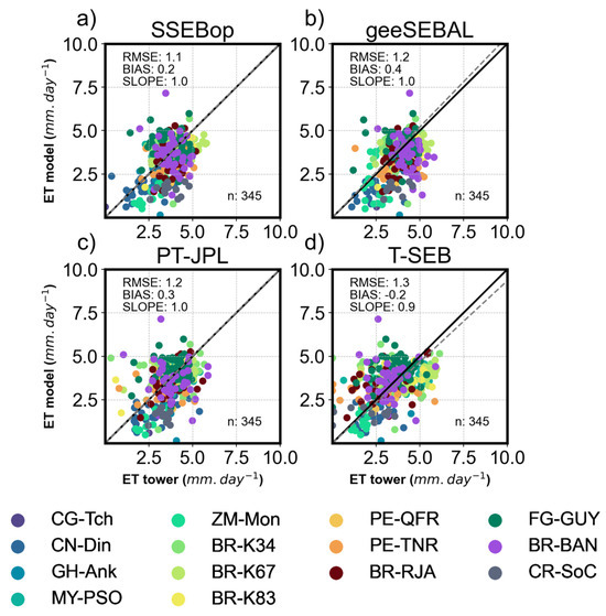
Figure 2. Comparison of daily $ET$ estimates from four models against flux tower EC data at tropical forest sites. The dashed line indicates the 1:1 relationship. (a) The SSEBop model showed the strongest agreement, followed by (b) geeSEBAL, (c) PT-JPL and (d) T-SEB.

The analysis conducted by continent is presented in Figure 3. The lowest average errors between simulated and observed $ET$ were found in the American continent, where the models showed average error of −0.34 mm.day⁻¹ (geeSEBAL), −0.22 mm.day⁻¹ (SSEBop), −0.09 mm.day⁻¹ (PT-JPL) and 0.18 mm.day⁻¹ (T-SEB). Subsequently, Asia exhibited intermediate errors (PT-JPL: −0.46 mm.day⁻¹, geeSEBAL: −0.43 mm.day⁻¹, T-SEB: −0.25 mm.day⁻¹, SSEBop: −0.10 mm.day⁻¹). In contrast, the greatest deviations were observed in Africa, with average errors of −1.35 mm.day⁻¹ (PT-JPL), −0.95 mm.day⁻¹ (SSEBop), −0.81 mm.day⁻¹ (geeSEBAL) and −0.28 mm.day⁻¹ (T-SEB).

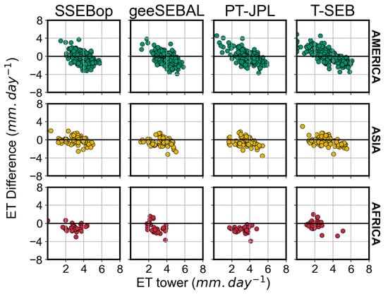
Figure 3. Relationship between $ET$ observed (x-axis) with the error difference (y-axis) for the four remote sensing models (SSEBop, PT-JPL, geeSEBAL and T-SEB), with data categorized by continent (the Americas, Asia and Africa).

3.2. Effect of Meteorological Input Data

The sensitivity of the four remote sensing models (SSEBop, geeSEBAL, PT-JPL and T-SEB) to four distinct meteorological datasets is summarized in Figure 4. The results revealed significant differences in models’ accuracy, highlighting systematic bias, and overall sensitivity to the input meteorological data. In terms of overall accuracy, the $RMSE$ values for most model-forcing combinations ranged between 1.1 and 1.9 mm.day⁻¹.

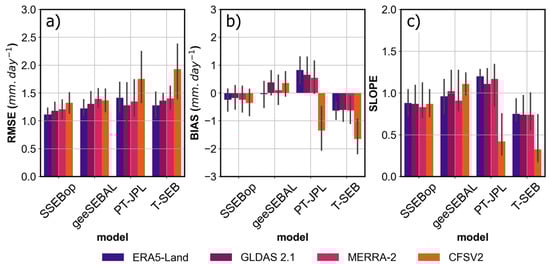
Figure 4. Boxplots of Root Mean Square Error (RMSE) (a), BIAS (b) and SLOPE (c) for the SSEBop, geeSEBAL, PT-JPL and T-SEB models using four different meteorological forcings.

The SSEBop and geeSEBAL models demonstrated the lowest sensitivity to the choice of meteorological input. In particular, SSEBop was the most robust, with $RMSE$ varying only between 1.1 mm.day⁻¹ (ERA5-Land) to 1.4 mm.day⁻¹ (CSFV2). Similarly, the geeSEBAL model also demonstrated a balanced performance, with low dependence of the meteorological forcing, as observed by previously studies [76,77]. Its $RMSE$ and $BIAS$, regardless of the meteorological forcing, yielded $RMSEs$ of 1.2, 1.3, 1.4 and 1.5 mm.day⁻¹, and $BIAS$ of −0.1, 0.4, −0.1 and 0.3 mm.day⁻¹ for ERA5-Land, GLDAS 2.1, MERRA-2 and CFSV2, respectively.

Conversely, the PT-JPL and T-SEB models showed greater sensitivity and systematic errors. PT-JPL persistently overestimated $ET$, showing a positive BIAS with three of the four inputs: ERA5-Land (0.82 mm.day⁻¹), GLDAS 2.1 (0.62 mm.day⁻¹) and MERRA-2 (0.58 mm.day⁻¹). The performance of both PT-JPL and T-SEB was substantially degraded when using CFSV2, which caused substantial underestimations with an average BIAS of −1.1 mm.day⁻¹ and −1.6 mm.day⁻¹, respectively.

3.3. Spatial–Temporal Response of ET to Tropical Deforestation

Figure 5 illustrates the spatial–temporal impacts of deforestation on daily $ET$ in three distinct tropical forest regions: the Amazon in Brazil (Figure 5a), the Congo forest in Zambia (Figure 5b) and Southeast Asian forest in Cambodia (Figure 5c). For each region, we performed a direct comparison between two specific Landsat scenes: an ‘intact’ scene from a period of extensive forest cover (before 1990) and a ‘deforested’ scene from a recent period (2024). To ensure the comparison primarily captured the effects of land-use change, the scenes were selected under similar climatic and seasonal conditions (dry season). The initial scenes are characterized by relatively homogeneous forests, with models generally exhibiting high $ET$ values and relative agreement with one another. However, in some scenarios, models diverged when assessing the impact of deforestation on $ET$.

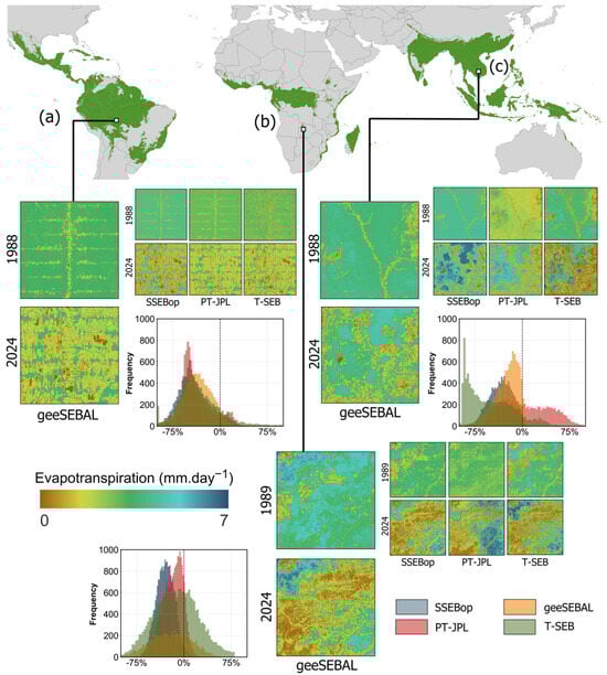
Figure 5. Impact of deforestation on daily $ET$ across three distinct tropical forest regions: (a) the Amazon (Brazil); (b) the Congo forest (Zambia); and (c) Southeast Asia (Cambodia). Landsat scenes from a period with homogeneous and intact forest cover were compared with more recent land-use conditions. Results were estimated by the four models (geeSEBAL, SSEBop, PT-JPL and T-SEB). The frequency plots illustrate the distribution of percentage change in $ET$ for all the models, calculated for each pixel.

In the Amazon site (Figure 5a), the assessed area (nearly 1000 km²) experienced a 79% increase in large, contiguous deforestation, with land converted into pasture and croplands. In this region, all models showed high agreement on the resulting impact. The distribution of percentage $ET$ change between the scenes was toward negative values for all four models, peaking between −25% and −50%. The mean reductions were larger for SSEBop and geeSEBAL models (approx. −44%) than PT-JPL (−40%) and T-SEB (−39%).

In contrast, the deforestation patterns in the African and Southeast Asian examples consist of smaller, fragmented forests. This fragmentation results in a more diffuse and generalized decrease in $ET$, which consequently appears to hinder the models’ consensus. For instance, results from the Congo site (Figure 5b) exhibited a less pronounced effect of deforestation on $ET$, despite deforested areas representing 42% of the site. The comparison between scenes showed that SSEBop demonstrated the highest sensitivity to the land-use change, with an average $ET$ reduction of −21%. This was followed by geeSEBAL (−13%), T-SEB (−10%) and PT-JPL (−8%). This particular result may be attributed to the diffuse, fragmented deforestation and a greater presence of forests, which all models showed having a positive $ET$ increase between scenes.

The most pronounced divergence between the models was observed in the Southeast Asian example (Figure 5c), where deforested areas increased by 46%. Here, the T-SEB, geeSEBAL and SSEBop models demonstrated a decrease in average $ET$ between the scenes. T-SEB showed a 58% reduction, followed by geeSEBAL (−21%) and SSEBop (−33%), while PT-JPL showed mixed results. These disagreements are a clear example of how different models’ assumptions and parametrizations within the model can produce divergent scenarios for impacts of deforestation using the same input data, particularly in regions characterized by fragmented land cover change.

3.4. Long-Term Impacts of Deforestation on ET

To illustrate the long-term impact of deforestation, we conducted a detailed times-series analysis (1985–2024) focused specifically on an Amazon site (Figure 6). This site was selected for the long-term analysis due to the availability of clear-sky images and annual land-use and cover classification data from the MapBiomas project [78], which is specific to Brazil.

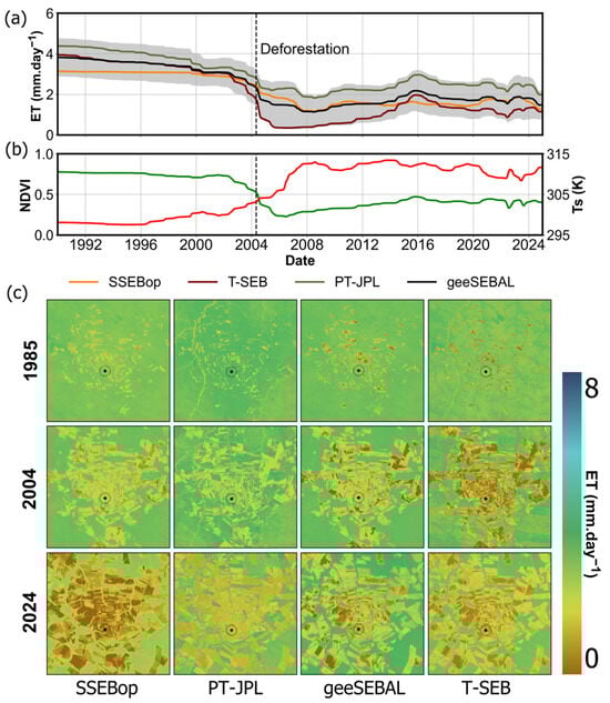
Figure 6. Temporal and spatial response of $ET$ to a deforestation timeline. (a) Displays the time series of average daily $ET$ from 1985 to 2024 using a low-filtering (gaussian filter) to evident the difference trends between before (1985) and after (2004) deforestation, as identified by the dashed line. The lines represent daily $ET$ for SSEBop (orange), T-SEB (brown), PT-JPL (green) and geeSEBAL (black), with corresponding shaded areas showing the standard deviation between models. (b) Time series of $NDVI$ (green) and $T_s$ (red). (c) Spatial distribution of daily $ET$ for the years 1985, 2004, and 2024, highlighting land use and land cover changes. The black marker indicates the specific point area used for the time series extraction in panels (a,b).

The analysis compared the $ET$ results for each of the four models. The MapBiomas data confirms that a major land cover change from forest to pasture and croplands occurred in this location, primarily after 2004. A gaussian filter was used to highlight the change between a forested state (1985) and a deforested state (post-2004).

Before deforestation, $ET$ rates were relatively stable and high, with the lowest values obtained by SSEBop (between 3.0 and 3.2 mm.day⁻¹), and the highest values by PT-JPL (between 3.2 and 4.3 mm.day⁻¹). For T-SEB and geeSEBAL, values ranged between 2.0 mm.day⁻¹ and 3.9 mm.day⁻¹, and 2.5 mm.day⁻¹ and 4.0 mm.day⁻¹, respectively.

A significant decline was observed after 2004, coinciding with the land cover conversion. The average $ET$ after deforestation showed lower values and higher variability due to seasonal variability, varying between 0.5 mm.day⁻¹ and 3.4 mm.day⁻¹, remaining at this lower level in the subsequent years. The T-SEB model showed the largest decrease (1.5 mm.day⁻¹), which suggests a high sensitivity to changes in land-use conditions. SSEBop and geeSEBAL showed similar sensitivity to the perturbation, decreasing substantially $ET$, and varying between 1.2 mm.day⁻¹ and 3.2 mm.day⁻¹. For PT-JPL, $ET$ results showed the least sensitivity to the land-use cover change, with a decrease of approximately 0.6 mm.day⁻¹.

4. Discussion

4.1. Models’ Performance and Spatial Patterns

Our assessment demonstrated that current remote sensing-based $ET$ models have reliable accuracy for tropical forests, which are comparable to that for other ecosystems when validated against EC data. However, the performance of these models over tropical forests using high-resolution imagery has rarely been examined, and such studies have typically concentrated on the Amazon region [79,80,81,82]. Studies in these areas commonly use coarse-resolution data (e.g., MODIS) [82,83,84,85,86], as such data are more widely available than high resolution $ET$ data [87].

For example, Moreira et al. [83] evaluated the accuracy of global $ET$ products (GLEAM, MOD16) against EC data in South America and reported an uncertainty between 18% and 22% for Amazon sites. Similarly, Paca et al. [84], comparing SSEBop results with MODIS for Amazon, obtained an average $RMSE$ of 0.8 mm.day⁻¹, while Alemayehu et al. [85] reported an error of 9.2% for the model over dense evergreen forest in Africa. Conversely, Bai [86] found a positive bias (13%) for the PT-JPL model in Chinese forests, while our study obtained similar results (11%) for a nearby location (CN-Din site).

Compared to results using Landsat data, Ghisi et al. [88] applied the T-SEB model over forest sites and reported an average $RMSE$ of 1.1 mm.day⁻¹, which is similar to our findings (1.3 mm.day⁻¹). Furthermore, Numata et al. [89], using the METRIC model [67] at the BR-RJA site, found an $RMSE$ of 0.8 mm.day⁻¹. This is comparable to what we found here using geeSEBAL (0.9 mm.day⁻¹), as these two models share similar assumptions, including the automatic endmembers selection [66].

Regarding spatial patterns, Khand et al. [90], using the METRIC model, found that deforestation resulted in a $ET$ decrease of approximately 1 mm.day⁻¹ for pasture sites compared to forests during the dry season. Similarly, Silva et al. [91], using coarse-resolution $ET$ data, found a 28% $ET$ reduction between forested and deforested areas from 2000 to 2014 in Rondônia state (Brazil), which is less than we found in Figure 5 between 1988 and 2024. In a study using geeSEBAL model and Landsat data, Laipelt et al. [76] found a long-term $ET$ decrease of 0.8 mm.day⁻¹ following deforestation near BR-BAN site.

4.2. Uncertainties in Monitoring Tropical Forest ET with Remote Sensing

Monitoring tropical forests at high spatial and temporal resolutions remains a fundamental challenge in remote sensing. First, extensive cloud cover in these humid regions severely limits the availability of clear-sky imagery, which can affect long-term analysis, and also introducing systematic biases on land surface temperature [60,92]. As illustrated in Figure 7, for much of the year the availability of clear-sky imagery (e.g., less than 50% cloud cover) is severely limited. This problem is particularly worsened during the wet season, such as from May to August in the Amazon and tropical Asia.

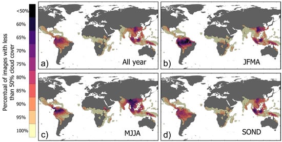
Figure 7. Seasonal and annual (a) percentage of available satellite images with less than 50% cloud cover. The presence of persistent cloud cover (indicated by warmer colors) significantly reduces the number of usable observations for $ET$ remote sensing analysis throughout the year and within specific seasons (JFMA (b), MJJA (c), SOND (d)).

Second, meteorological forcing is highly influential on the accuracy of $ET$ models [93,94]. This issue is exacerbated in tropical areas due to a lower density of in situ weather stations compared to mid-latitude regions [70,95] and cloud cover [69]. Consequently, there is a higher reliance on satellite-derived and reanalysis products, which can introduce systematic biases. Nevertheless, the data quality of reanalysis products over tropical areas has the potential to introduce significant biases in $ET$ results. Gomis-Cebolla et al. [79] evaluated MERRA, ERA5 and GLDAS datasets’ influence on global $ET$ models in the Amazon comparing against EC site data, finding significant discrepancies between models’ estimates. Moreover, a scale mismatch often exists between meteorological products and satellite imagery [96]. This discrepancy can degrade model performance by poorly representing key local variables such as air temperature, relative humidity and radiation.

In this study, different models exhibited sensitivity to these meteorological inputs. We found that geeSEBAL and SSEBop showed the lowest sensitivity, whereas PT-JPL and T-SEB showed the highest. The sensitivity of the PT-JPL model to radiation inputs was described by Fisher et al. [64] and has been confirmed by other studies [97]. Similarly, because T-SEB models’ parameterization is fundamentally driven by the interplay between $T_{rad}$ and near-surface atmospheric conditions, biases in meteorological inputs can significantly impact model performance [98]. Notably, the ERA5-Land meteorological dataset yielded the highest model accuracy, and has been successfully utilized for remote sensing $ET$ predictions [99,100].

In contrast, the CFSv2 dataset consistently yielded the poorest results. This is likely due to its coarse spatial (~0.5°) and temporal resolution (6-hourly), limiting the ability to capture local heterogeneity in temperature, humidity and radiation.

4.3. Remote Sensing Estimation of ET for Tropical Forests Monitoring

Satellites are the only viable alternative to continuously monitoring tropical forests and their contribution to regional climate. While high-resolution surface data have limited temporal rate [101], there are initiatives aiming at overcoming these gaps. For instance, combining different satellite datasets to improve high-temporal coverage [102,103,104,105] holds significant potential for tropical regions. For instance, the Harmonized Landsat-Sentinel product combines and harmonizes observations of both satellites to increase data frequency [106]. A major limitation, however, persists, as the thermal band is an essential input for most $ET$ models and is not available for Sentinel-2. Though other sensors provide more frequent thermal data (e.g., MODIS, VIIRS), their coarse spatial resolution (typically 1 km) limits their use for local-scale $ET$ monitoring [101]. To address this, many studies have focused on methods to enhance the spatial resolution of coarse $T_{rad}$ [107,108,109]. Despite being promising, these approaches have typically been applied over small, specific areas, with a notable lack of research in tropical areas.

As illustrated in Figure 8 for a deforested area in the Brazilian Amazon, coarse-resolution data fail to represent the complex, patchy nature of tropical deforestation. The 1000 m MOD16 data, for example, average the $ET$ signal over a large pixel (1 km²). This aggregation reduces the $ET$ response by mixing the surface signals, consequently becoming representative of neither the deforested patches nor the surrounding intact forest. In contrast, the 30 m high-resolution ensemble of the four $ET$ models evaluated in this study (Figure 8) demonstrates the capacity to represent deforestation patches by capturing the fine-scale spatial variations over deforested areas, as well as the $ET$ gradient between the drier, deforested land and the wet surrounding forest.

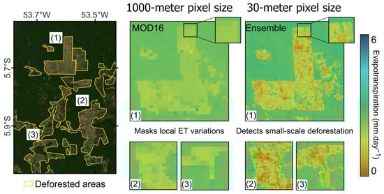
Figure 8. $ET$ estimates for a deforested area at different spatial resolutions, showing the effect of pixel size on mapping $ET$. Results obtained with MOD16 mask local $ET$ variations due to an inadequate pixel size to monitor complex local deforestation patches. In contrast, the ensemble average of the $ET$ models (geeSEBAL, PT-JPL, SSEBop and T-SEB) successfully detected small-scale $ET$ variations over the deforested areas.

Upcoming satellite missions are set to significantly benefit $ET$ monitoring by increasing the frequency of globally available observations. Public initiatives such as TRISHNA (Thermal infrared Imaging Satellite for High resource Assessment) [110] and Landsat Next [111] are expected to enhance global monitoring of Earth’s surface, greatly improving our understanding of ecosystems changes. In the private sector, Hydrosat [112] plans to launch a constellation of satellites that will provide daily high-resolution thermal and multispectral data. Furthermore, integrating radar data from missions like Sentinel-1 and the upcoming NISAR (NASA-ISRO Synthetic Aperture Radar) mission [113] has the potential to overcome the persistent issue of cloud cover in tropical regions [110,114,115]. Alterations in the radar signal can be directly correlated with vegetation changes, such as deforestation, and variations in soil moisture content [111,112,113], although assimilation with $ET$ models is still needed.

Lastly, the current state and position of remote sensing $ET$ modeling enable the development of platforms dedicated to continuously monitoring $ET$ in tropical areas with satellite data. Prominent examples include OpenET [41], which offers $ET$ data for the western United States and aims to expand to global coverage [114], and FAO’s WaPOR [115], which provides historical $ET$ data with a focus on the African continent. A global, high-resolution $ET$ platform with multiple models would democratize access to accurate information, thereby enhancing our understanding of $ET$ processes.

5. Conclusions

In this study, a comprehensive assessment of four remote sensing-based $ET$ models was provided for global tropical forests. Models’ performance was evaluated by comparing daily $ET$ estimates against EC data carried out in 14 sites, distributed along nine countries. Results showed that the evaluated models yielded similar performance metrics and effectively represented $ET$ over tropical forests. Conversely, their behavior diverged when subjected to different meteorological inputs and deforestation scenarios. The ERA5-Land and GLDAS 2.1 datasets consistently provided the most accurate inputs for all four models, while CFSV2 was associated with the highest uncertainties.

The analysis of deforestation impacts revealed distinct models’ sensitivities. The magnitude of the $ET$ decrease due to deforestation depended on the specific deforestation patterns at each site, varying between the evaluated sites. In addition, the long-term $ET$ changes showed that PT-JPL demonstrated the least responsive to land cover shifts (−0.6 mm.day⁻¹), while T-SEB demonstrated the greatest sensitivity to change (1.5 mm.day⁻¹).

Our findings increase the understanding of the benefits and limitations of applying different high-resolution $ET$ models in these areas. By demonstrating their reliability, this study confirms that these models are valuable tools for assessing the forest’s contribution to water flux circulation and potential impacts of deforestation, which can significantly support regional conservations’ efforts. Future research should incorporate additional datasets, such as Sentinel-2 satellite imagery, coupled with downscaling methods. This approach will improve spatial and temporal resolution, enabling more detailed and continuous observations of these globally important ecosystems.

References

- Spracklen, D.V.; Arnold, S.R.; Taylor, C.M. Observations of Increased Tropical Rainfall Preceded by Air Passage over Forests. Nature 2012, 489, 282–285. [Google Scholar] [CrossRef] [PubMed]
- Bonan, G.B. Forests and Climate Change: Forcings, Feedbacks, and the Climate Benefits of Forests. Science 2008, 320, 1444–1449. [Google Scholar] [CrossRef] [PubMed]
- Dyer, E.L.E.; Jones, D.B.A.; Nusbaumer, J.; Li, H.; Collins, O.; Vettoretti, G.; Noone, D. Congo Basin Precipitation: Assessing Seasonality, Regional Interactions, and Sources of Moisture. J. Geophys. Res. Atmos. 2017, 122, 6882–6898. [Google Scholar] [CrossRef]
- Aragão, L. The Rainforest’s Water Pump. Nature 2012, 489, 217–218. [Google Scholar] [CrossRef]
- Spracklen, D.V.; Garcia-Carreras, L. The Impact of Amazonian Deforestation on Amazon Basin Rainfall. Geophys. Res. Lett. 2015, 42, 9546–9552. [Google Scholar] [CrossRef]
- Bierregaard, R.O.; Lovejoy, T.E.; Kapos, V.; dos Santos, A.A.; Hutchings, R.W. The Biological Dynamics of Tropical Rainforest Fragments. Bioscience 1992, 42, 859–866. [Google Scholar] [CrossRef]
- Schlesinger, W.H.; Jasechko, S. Transpiration in the Global Water Cycle. Agric. For. Meteorol. 2014, 189–190, 115–117. [Google Scholar] [CrossRef]
- van der Ent, R.J.; Wang-Erlandsson, L.; Keys, P.W.; Savenije, H.H.G. Contrasting Roles of Interception and Transpiration in the Hydrological Cycle—Part 2: Moisture Recycling. Earth Syst. Dyn. 2014, 5, 471–489. [Google Scholar] [CrossRef]
- Burnett, M.W.; Quetin, G.R.; Konings, A.G. Data-Driven Estimates of Evapotranspiration and Its Controls in the Congo Basin. Hydrol. Earth Syst. Sci. 2020, 24, 4189–4211. [Google Scholar] [CrossRef]
- Alves de Oliveira, B.F.; Bottino, M.J.; Nobre, P.; Nobre, C.A. Deforestation and Climate Change Are Projected to Increase Heat Stress Risk in the Brazilian Amazon. Commun. Earth Environ. 2021, 2, 207. [Google Scholar] [CrossRef]
- Cooley, S.S.; Keller, M.; Longo, M.; Csillik, O.; Dias, A.P.; Silgueiro, V.; Carvalho, R.; Anderson, D.; Gilbreath, M.; Duffy, P.; et al. Thermal Stress in Degraded Forests in the Brazilian Amazon Arc of Deforestation. Environ. Res. Lett. 2025, 20, 084069. [Google Scholar] [CrossRef]
- Berenguer, E.; Lennox, G.D.; Ferreira, J.; Malhi, Y.; Aragão, L.E.O.C.; Barreto, J.R.; Del Bon Espírito-Santo, F.; Figueiredo, A.E.S.; França, F.; Gardner, T.A.; et al. Tracking the Impacts of El Niño Drought and Fire in Human-Modified Amazonian Forests. Proc. Natl. Acad. Sci. USA 2021, 118, e2019377118. [Google Scholar] [CrossRef] [PubMed]
- Van Nieuwstadt, M.G.L.; Sheil, D. Drought, Fire and Tree Survival in a Borneo Rain Forest, East Kalimantan, Indonesia. J. Ecol. 2005, 93, 191–201. [Google Scholar] [CrossRef]
- de Oliveira Silva, R.; Barioni, L.G.; Hall, J.A.J.; Folegatti Matsuura, M.; Zanett Albertini, T.; Fernandes, F.A.; Moran, D. Increasing Beef Production Could Lower Greenhouse Gas Emissions in Brazil If Decoupled from Deforestation. Nat. Clim. Change 2016, 6, 493–497. [Google Scholar] [CrossRef]
- Giljum, S.; Maus, V.; Kuschnig, N.; Luckeneder, S.; Tost, M.; Sonter, L.J.; Bebbington, A.J. A Pantropical Assessment of Deforestation Caused by Industrial Mining. Proc. Natl. Acad. Sci. USA 2022, 119, e2118273119. [Google Scholar] [CrossRef]
- Skidmore, M.E.; Moffette, F.; Rausch, L.; Christie, M.; Munger, J.; Gibbs, H.K. Cattle Ranchers and Deforestation in the Brazilian Amazon: Production, Location, and Policies. Glob. Environ. Change 2021, 68, 102280. [Google Scholar] [CrossRef]
- Lawrence, D.; Vandecar, K. Effects of Tropical Deforestation on Climate and Agriculture. Nat. Clim. Change 2015, 5, 27–36. [Google Scholar] [CrossRef]
- Paul, S.; Ghosh, S.; Oglesby, R.; Pathak, A.; Chandrasekharan, A.; Ramsankaran, R. Weakening of Indian Summer Monsoon Rainfall Due to Changes in Land Use Land Cover. Sci. Rep. 2016, 6, 32177. [Google Scholar] [CrossRef]
- Sen, O.L.; Wang, Y.; Wang, B. Impact of Indochina Deforestation on the East Asian Summer Monsoon. J. Clim. 2004, 17, 1366–1380. [Google Scholar] [CrossRef]
- Knox, R.; Bisht, G.; Wang, J.; Bras, R. Precipitation Variability over the Forest-to-Nonforest Transition in Southwestern Amazonia. J. Clim. 2011, 24, 2368–2377. [Google Scholar] [CrossRef]
- Mu, Y.; Jones, C. An Observational Analysis of Precipitation and Deforestation Age in the Brazilian Legal Amazon. Atmos. Res. 2022, 271, 106122. [Google Scholar] [CrossRef]
- Paiva, R.C.D.; Buarque, D.C.; Clarke, R.T.; Collischonn, W.; Allasia, D.G. Reduced Precipitation over Large Water Bodies in the Brazilian Amazon Shown from TRMM Data. Geophys. Res. Lett. 2011, 38, L045277. [Google Scholar] [CrossRef]
- Heerspink, B.P.; Kendall, A.D.; Coe, M.T.; Hyndman, D.W. Trends in Streamflow, Evapotranspiration, and Groundwater Storage across the Amazon Basin Linked to Changing Precipitation and Land Cover. J. Hydrol. Reg. Stud. 2020, 32, 100755. [Google Scholar] [CrossRef]
- Hirano, T.; Kusin, K.; Limin, S.; Osaki, M. Evapotranspiration of Tropical Peat Swamp Forests. Glob. Change Biol. 2015, 21, 1914–1927. [Google Scholar] [CrossRef] [PubMed]
- Bell, J.P.; Tompkins, A.M.; Bouka-Biona, C.; Sanda, I.S. A Process-Based Investigation into the Impact of the Congo Basin Deforestation on Surface Climate. J. Geophys. Res. Atmos. 2015, 120, 5721–5739. [Google Scholar] [CrossRef]
- Reddington, C.L.; Smith, C.; Butt, E.W.; Baker, J.C.A.; Oliveira, B.F.A.; Yamba, E.I.; Spracklen, D.V. Tropical Deforestation Is Associated with Considerable Heat-Related Mortality. Nat. Clim. Change 2025, 15, 992–999. [Google Scholar] [CrossRef]
- Nobre, C.A.; Sampaio, G.; Borma, L.S.; Castilla-Rubio, J.C.; Silva, J.S.; Cardoso, M. Land-Use and Climate Change Risks in the Amazon and the Need of a Novel Sustainable Development Paradigm. Proc. Natl. Acad. Sci. USA 2016, 113, 10759–10768. [Google Scholar] [CrossRef]
- Borma, L.S.; Costa, M.H.; da Rocha, H.R.; Arieira, J.; Nascimento, N.C.C.; Jaramillo-Giraldo, C.; Ambrosio, G.; Carneiro, R.G.; Venzon, M.; Neto, A.F.; et al. Beyond Carbon: The Contributions of South American Tropical Humid and Subhumid Forests to Ecosystem Services. Rev. Geophys. 2022, 60, e2021RG000766. [Google Scholar] [CrossRef]
- Smith, C.; Baker, J.C.A.; Spracklen, D.V. Tropical Deforestation Causes Large Reductions in Observed Precipitation. Nature 2023, 615, 270–275. [Google Scholar] [CrossRef]
- Flores, B.M.; Montoya, E.; Sakschewski, B.; Nascimento, N.; Staal, A.; Betts, R.A.; Levis, C.; Lapola, D.M.; Esquível-Muelbert, A.; Jakovac, C.; et al. Critical Transitions in the Amazon Forest System. Nature 2024, 626, 555–564. [Google Scholar] [CrossRef]
- Biscaro, T.S.; Machado, L.A.T.; Giangrande, S.E.; Jensen, M.P. What Drives Daily Precipitation over the Central Amazon? Differences Observed between Wet and Dry Seasons. Atmos. Chem. Phys. 2021, 21, 6735–6754. [Google Scholar] [CrossRef]
- Vergopolan, N.; Fisher, J.B. The Impact of Deforestation on the Hydrological Cycle in Amazonia as Observed from Remote Sensing. Int. J. Remote Sens. 2016, 37, 5412–5430. [Google Scholar] [CrossRef]
- Khanna, J.; Medvigy, D. Strong Control of Surface Roughness Variations on the Simulated Dry Season Regional Atmospheric Response to Contemporary Deforestation in Rondônia, Brazil. J. Geophys. Res. Atmos. 2014, 119, 13067–13078. [Google Scholar] [CrossRef]
- Baldocchi, D.; Falge, E.; Gu, L.; Olson, R.; Hollinger, D.; Running, S.; Anthoni, P.; Bernhofer, C.; Davis, K.; Evans, R.; et al. FLUXNET: A New Tool to Study the Temporal and Spatial Variability of Ecosystem-Scale Carbon Dioxide, Water Vapor, and Energy Flux Densities. Bull. Am. Meteorol. Soc. 2001, 82, 2415–2434. [Google Scholar] [CrossRef]
- Yuan, K.; Zhu, Q.; Zheng, S.; Zhao, L.; Chen, M.; Riley, W.J.; Cai, X.; Ma, H.; Li, F.; Wu, H.; et al. Deforestation Reshapes Land-Surface Energy-Flux Partitioning. Environ. Res. Lett. 2021, 16, 024014. [Google Scholar] [CrossRef]
- Jaafar, H.H.; Ahmad, F.A. Time Series Trends of Landsat-Based ET Using Automated Calibration in METRIC and SEBAL: The Bekaa Valley, Lebanon. Remote Sens. Environ. 2020, 238, 111034. [Google Scholar] [CrossRef]
- Ferguson, C.R.; Sheffield, J.; Wood, E.F.; Gao, H. Quantifying Uncertainty in a Remote Sensing-Based Estimate of Evapotranspiration over Continental USA. Int. J. Remote Sens. 2010, 31, 3821–3865. [Google Scholar] [CrossRef]
- French, A.N.; Hunsaker, D.J.; Thorp, K.R. Remote Sensing of Evapotranspiration over Cotton Using the TSEB and METRIC Energy Balance Models. Remote Sens. Environ. 2015, 158, 281–294. [Google Scholar] [CrossRef]
- Nagler, P. The Role of Remote Sensing Observations and Models in Hydrology: The Science of Evapotranspiration. Hydrol. Process. 2011, 25, 3977–3978. [Google Scholar] [CrossRef]
- McShane, R.R.; Driscoll, K.P.; Sando, R. A Review of Surface Energy Balance Models for Estimating Actual Evapotranspiration with Remote Sensing at High Spatiotemporal Resolution over Large Extents; United States Geological Survey: Reston, VA, USA, 2017.
- Melton, F.S.; Huntington, J.; Grimm, R.; Herring, J.; Hall, M.; Rollison, D.; Erickson, T.; Allen, R.; Anderson, M.; Fisher, J.B.; et al. OpenET: Filling a Critical Data Gap in Water Management for the Western United States. JAWRA J. Am. Water Resour. Assoc. 2022, 58, 971–994. [Google Scholar] [CrossRef]
- Bastiaanssen, W.G.M.; Menenti, M.; Feddes, R.A.; Holtslag, A.A.M. A Remote Sensing Surface Energy Balance Algorithm for Land (SEBAL): 1. Formulation. J. Hydrol. 1998, 212–213, 198–212. [Google Scholar] [CrossRef]
- Allen, R.G.; Tasumi, M.; Trezza, R. Satellite-Based Energy Balance for Mapping Evapotranspiration with Internalized Calibration (METRIC)—Model. J. Irrig. Drain. Eng. 2007, 133, 380–394. [Google Scholar] [CrossRef]
- Wilson, K.; Goldstein, A.; Falge, E.; Aubinet, M.; Baldocchi, D.; Berbigier, P.; Bernhofer, C.; Ceulemans, R.; Dolman, H.; Field, C.; et al. Energy Balance Closure at FLUXNET Sites. Agric. For. Meteorol. 2002, 113, 223–243. [Google Scholar] [CrossRef]
- Twine, T.E.; Kustas, W.P.; Norman, J.M.; Cook, D.R.; Houser, P.R.; Meyers, T.P.; Prueger, J.H.; Starks, P.J.; Wesely, M.L. Correcting Eddy-Covariance Flux Underestimates over a Grassland. Agric. For. Meteorol. 2000, 103, 279–300. [Google Scholar] [CrossRef]
- Borma, L.S.; da Rocha, H.R.; Cabral, O.M.; von Randow, C.; Collicchio, E.; Kurzatkowski, D.; Brugger, P.J.; Freitas, H.; Tannus, R.; Oliveira, L.; et al. Atmosphere and Hydrological Controls of the Evapotranspiration over a Floodplain Forest in the Bananal Island Region, Amazonia. J. Geophys. Res. 2009, 114, G01003. [Google Scholar] [CrossRef]
- Araújo, A.C.; Nobre, A.D.; Kruijt, B.; Elbers, J.A.; Dallarosa, R.; Stefani, P.; von Randow, C.; Manzi, A.O.; Culf, A.D.; Gash, J.H.C.; et al. Comparative Measurements of Carbon Dioxide Fluxes from Two Nearby Towers in a Central Amazonian Rainforest: The Manaus LBA Site. J. Geophys. Res. Atmos. 2002, 107, 8090. [Google Scholar] [CrossRef]
- Saleska, S.R.; Da Rocha, H.R.; Huete, A.R.; Nobre, A.D.; Artaxo, P.E.; Shimabukuro, Y.E. LBA-ECO CD-32 Flux Tower Network Data Compilation, Brazilian Amazon: 1999–2006; ORNL DAAC: Oak Ridge, TN, USA, 2013.
- da Rocha, H.R.; Goulden, M.L.; Miller, S.D.; Menton, M.C.; Pinto, L.D.V.O.; de Freitas, H.C.; e Silva Figueira, A.M. Seasonality of Water and Heat Fluxes over a Tropical Forest In Eastern Amazonia. Ecol. Appl. 2004, 14, 22–32. [Google Scholar] [CrossRef]
- von Randow, C.; Manzi, A.O.; Kruijt, B.; de Oliveira, P.J.; Zanchi, F.B.; Silva, R.L.; Hodnett, M.G.; Gash, J.H.C.; Elbers, J.A.; Waterloo, M.J.; et al. Comparative Measurements and Seasonal Variations in Energy and Carbon Exchange over Forest and Pasture in South West Amazonia. Theor. Appl. Climatol. 2004, 78, 5–26. [Google Scholar] [CrossRef]
- Merbold, L.; Ardö, J.; Arneth, A.; Scholes, R.J.; Nouvellon, Y.; de Grandcourt, A.; Archibald, S.; Bonnefond, J.M.; Boulain, N.; Brueggemann, N.; et al. Precipitation as Driver of Carbon Fluxes in 11 African Ecosystems. Biogeosciences 2009, 6, 1027–1041. [Google Scholar] [CrossRef]
- Yu, G.-R.; Wen, X.-F.; Sun, X.-M.; Tanner, B.D.; Lee, X.; Chen, J.-Y. Overview of ChinaFLUX and Evaluation of Its Eddy Covariance Measurement. Agric. For. Meteorol. 2006, 137, 125–137. [Google Scholar] [CrossRef]
- Aparecido, L.M.T.; Miller, G.R.; Cahill, A.T.; Moore, G.W. Leaf Surface Traits and Water Storage Retention Affect Photosynthetic Responses to Leaf Surface Wetness among Wet Tropical Forest and Semiarid Savanna Plants. Tree Physiol. 2017, 37, 1285–1300. [Google Scholar] [CrossRef] [PubMed]
- Bonal, D.; Bosc, A.; Ponton, S.; Goret, J.; Burban, B.; Gross, P.; Bonnefond, J.; Elbers, J.; Longdoz, B.; Epron, D.; et al. Impact of Severe Dry Season on Net Ecosystem Exchange in the Neotropical Rainforest of French Guiana. Glob. Change Biol. 2008, 14, 1917–1933. [Google Scholar] [CrossRef]
- Chiti, T.; Certini, G.; Grieco, E.; Valentini, R. The Role of Soil in Storing Carbon in Tropical Rainforests: The Case of Ankasa Park, Ghana. Plant Soil 2010, 331, 453–461. [Google Scholar] [CrossRef]
- Kosugi, Y.; Mitani, T.; Itoh, M.; Noguchi, S.; Tani, M.; Matsuo, N.; Takanashi, S.; Ohkubo, S.; Rahim Nik, A. Spatial and Temporal Variation in Soil Respiration in a Southeast Asian Tropical Rainforest. Agric. For. Meteorol. 2007, 147, 35–47. [Google Scholar] [CrossRef]
- Griffis, T.J.; Roman, D.T.; Wood, J.D.; Deventer, J.; Fachin, L.; Rengifo, J.; Del Castillo, D.; Lilleskov, E.; Kolka, R.; Chimner, R.A.; et al. Hydrometeorological Sensitivities of Net Ecosystem Carbon Dioxide and Methane Exchange of an Amazonian Palm Swamp Peatland. Agric. For. Meteorol. 2020, 295, 108167. [Google Scholar] [CrossRef]
- Vihermaa, L.E.; Waldron, S.; Domingues, T.; Grace, J.; Cosio, E.G.; Limonchi, F.; Hopkinson, C.; da Rocha, H.R.; Gloor, E. Fluvial Carbon Export from a Lowland Amazonian Rainforest in Relation to Atmospheric Fluxes. J. Geophys. Res. Biogeosci. 2016, 121, 3001–3018. [Google Scholar] [CrossRef]
- Ermida, S.L.; Trigo, I.F.; DaCamara, C.C.; Jiménez, C.; Prigent, C. Quantifying the Clear-Sky Bias of Satellite Land Surface Temperature Using Microwave-Based Estimates. J. Geophys. Res. Atmos. 2019, 124, 844–857. [Google Scholar] [CrossRef]
- Senay, G.B. Satellite Psychrometric Formulation of the Operational Simplified Surface Energy Balance (SSEBop) Model for Quantifying and Mapping Evapotranspiration. Appl. Eng. Agric. 2018, 34, 555–566. [Google Scholar] [CrossRef]
- Senay, G.B.; Kagone, S.; Velpuri, N.M. Operational Global Actual Evapotranspiration: Development, Evaluation, and Dissemination. Sensors 2020, 20, 1915. [Google Scholar] [CrossRef]
- Senay, G.B.; Parrish, G.E.L.; Schauer, M.; Friedrichs, M.; Khand, K.; Boiko, O.; Kagone, S.; Dittmeier, R.; Arab, S.; Ji, L. Improving the Operational Simplified Surface Energy Balance Evapotranspiration Model Using the Forcing and Normalizing Operation. Remote Sens. 2023, 15, 260. [Google Scholar] [CrossRef]
- Fisher, J.B.; Tu, K.P.; Baldocchi, D.D. Global Estimates of the Land–Atmosphere Water Flux Based on Monthly AVHRR and ISLSCP-II Data, Validated at 16 FLUXNET Sites. Remote Sens. Environ. 2008, 112, 901–919. [Google Scholar] [CrossRef]
- Priestley, C.H.B.; Taylor, R.J. On the Assessment of Surface Heat Flux and Evaporation Using Large-Scale Parameters. Mon. Weather Rev. 1972, 100, 81–92. [Google Scholar] [CrossRef]
- Laipelt, L.; Kayser, R.H.B.; Fleischmann, A.S.; Ruhoff, A.; Bastiaanssen, W.; Erickson, T.A.; Melton, F. Long-Term Monitoring of Evapotranspiration Using the SEBAL Algorithm and Google Earth Engine Cloud Computing. ISPRS J. Photogramm. Remote Sens. 2021, 178, 81–96. [Google Scholar] [CrossRef]
- Allen, R.G.; Burnett, B.; Kramber, W.; Huntington, J.; Kjaersgaard, J.; Kilic, A.; Kelly, C.; Trezza, R. Automated Calibration of the METRIC-Landsat Evapotranspiration Process. JAWRA J. Am. Water Resour. Assoc. 2013, 49, 563–576. [Google Scholar] [CrossRef]
- Norman, J.M.; Kustas, W.P.; Humes, K.S. Source Approach for Estimating Soil and Vegetation Energy Fluxes in Observations of Directional Radiometric Surface Temperature. Agric. For. Meteorol. 1995, 77, 263–293. [Google Scholar] [CrossRef]
- Ukhurebor, K.E.; Azi, S.O.; Aigbe, U.O.; Onyancha, R.B.; Emegha, J.O. Analyzing the Uncertainties between Reanalysis Meteorological Data and Ground Measured Meteorological Data. Measurement 2020, 165, 108110. [Google Scholar] [CrossRef]
- Zhao, M.; Running, S.W.; Nemani, R.R. Sensitivity of Moderate Resolution Imaging Spectroradiometer (MODIS) Terrestrial Primary Production to the Accuracy of Meteorological Reanalyses. J. Geophys. Res. Biogeosci. 2006, 111, G01002. [Google Scholar] [CrossRef]
- Muñoz-Sabater, J.; Dutra, E.; Agustí-Panareda, A.; Albergel, C.; Arduini, G.; Balsamo, G.; Boussetta, S.; Choulga, M.; Harrigan, S.; Hersbach, H.; et al. ERA5-Land: A State-of-the-Art Global Reanalysis Dataset for Land Applications. Earth Syst. Sci. Data Discuss. 2021, 13, 4349–4383. [Google Scholar] [CrossRef]
- Saha, S.; Moorthi, S.; Wu, X.; Wang, J.; Nadiga, S.; Tripp, P.; Behringer, D.; Hou, Y.-T.; Chuang, H.; Iredell, M.; et al. The NCEP Climate Forecast System Version 2. J. Clim. 2014, 27, 2185–2208. [Google Scholar] [CrossRef]
- Rodell, M.; Houser, P.R.; Jambor, U.; Gottschalck, J.; Mitchell, K.; Meng, C.-J.; Arsenault, K.; Cosgrove, B.; Radakovich, J.; Bosilovich, M.; et al. The Global Land Data Assimilation System. Bull. Am. Meteorol. Soc. 2004, 85, 381–394. [Google Scholar] [CrossRef]
- Gelaro, R.; McCarty, W.; Suárez, M.J.; Todling, R.; Molod, A.; Takacs, L.; Randles, C.A.; Darmenov, A.; Bosilovich, M.G.; Reichle, R.; et al. The Modern-Era Retrospective Analysis for Research and Applications, Version 2 (MERRA-2). J. Clim. 2017, 30, 5419–5454. [Google Scholar] [CrossRef] [PubMed]
- Shuttleworth, W.J. Terrestrial Hydrometeorology; John Wiley & Sons, Ltd.: Chichester, UK, 2012; ISBN 9781119951933. [Google Scholar]
- Laipelt, L.; Ruhoff, L.A.; Fleischmann, S.A.; Kayser, H.R.; Kich, D.E.; da Rocha, R.H.; Neale, M.C. Assessment of an Automated Calibration of the SEBAL Algorithm to Estimate Dry-Season Surface-Energy Partitioning in a Forest–Savanna Transition in Brazil. Remote Sens. 2020, 12, 1108. [Google Scholar] [CrossRef]
- Long, D.; Singh, V.P.; Li, Z.-L. How Sensitive Is SEBAL to Changes in Input Variables, Domain Size and Satellite Sensor? J. Geophys. Res. Atmos. 2011, 116, D21107. [Google Scholar] [CrossRef]
- Gomis-Cebolla, J.; Jimenez, J.C.; Sobrino, J.A.; Corbari, C.; Mancini, M. Intercomparison of Remote-Sensing Based Evapotranspiration Algorithms over Amazonian Forests. Int. J. Appl. Earth Obs. Geoinf. 2019, 80, 280–294. [Google Scholar] [CrossRef]
- Maeda, E.E.; Ma, X.; Wagner, F.H.; Kim, H.; Oki, T.; Eamus, D.; Huete, A. Evapotranspiration Seasonality across the Amazon Basin. Earth Syst. Dyn. 2017, 8, 439–454. [Google Scholar] [CrossRef]
- Wu, J.; Lakshmi, V.; Wang, D.; Lin, P.; Pan, M.; Cai, X.; Wood, E.F.; Zeng, Z. The Reliability of Global Remote Sensing Evapotranspiration Products over Amazon. Remote Sens. 2020, 12, 2211. [Google Scholar] [CrossRef]
- da Silva, H.J.F.; Gonçalves, W.A.; Bezerra, B.G. Comparative Analyzes and Use of Evapotranspiration Obtained through Remote Sensing to Identify Deforested Areas in the Amazon. Int. J. Appl. Earth Obs. Geoinf. 2019, 78, 163–174. [Google Scholar] [CrossRef]
- Moreira, A.A.; Ruhoff, A.L.; Roberti, D.R.; Souza, V.d.A.; da Rocha, H.R.; de Paiva, R.C.D. Assessment of Terrestrial Water Balance Using Remote Sensing Data in South America. J. Hydrol. 2019, 575, 131–147. [Google Scholar] [CrossRef]
- Paca, V.H.d.M.; Espinoza-Dávalos, G.E.; Hessels, T.M.; Moreira, D.M.; Comair, G.F.; Bastiaanssen, W.G.M. The Spatial Variability of Actual Evapotranspiration across the Amazon River Basin Based on Remote Sensing Products Validated with Flux Towers. Ecol. Process. 2019, 8, 6. [Google Scholar] [CrossRef]
- Alemayehu, T.; van Griensven, A.; Senay, G.B.; Bauwens, W. Evapotranspiration Mapping in a Heterogeneous Landscape Using Remote Sensing and Global Weather Datasets: Application to the Mara Basin, East Africa. Remote Sens. 2017, 9, 390. [Google Scholar] [CrossRef]
- Bai, P. Comparison of Remote Sensing Evapotranspiration Models: Consistency, Merits, and Pitfalls. J. Hydrol. 2023, 617, 128856. [Google Scholar] [CrossRef]
- Castagna, D.; Barbosa, L.S.; Martim, C.C.; Paulista, R.S.D.; Machado, N.G.; Biudes, M.S.; de Souza, A.P. Evapotranspiration Assessment by Remote Sensing in Brazil with Focus on Amazon Biome: Scientometric Analysis and Perspectives for Applications in Agro-Environmental Studies. Hydrology 2024, 11, 39. [Google Scholar] [CrossRef]
- Pan, X.; Wang, Z.; Liu, S.; Yang, Z.; Guluzade, R.; Liu, Y.; Yuan, J.; Yang, Y. The Impact of Clear-Sky Biases of Land Surface Temperature on Monthly Evapotranspiration Estimation. Int. J. Appl. Earth Obs. Geoinf. 2024, 129, 103811. [Google Scholar] [CrossRef]
- Vinukollu, R.K.; Meynadier, R.; Sheffield, J.; Wood, E.F. Multi-Model, Multi-Sensor Estimates of Global Evapotranspiration: Climatology, Uncertainties and Trends. Hydrol. Process. 2011, 25, 3993–4010. [Google Scholar] [CrossRef]
- Long, D.; Longuevergne, L.; Scanlon, B.R. Uncertainty in Evapotranspiration from Land Surface Modeling, Remote Sensing, and GRACE Satellites. Water Resour. Res. 2014, 50, 1131–1151. [Google Scholar] [CrossRef]
- Clark, D.A. Tropical Forests and Global Warming: Slowing It down or Speeding It Up? Front. Ecol. Environ. 2004, 2, 73–80. [Google Scholar] [CrossRef]
- Yang, Y.; Long, D.; Shang, S. Remote Estimation of Terrestrial Evapotranspiration without Using Meteorological Data. Geophys. Res. Lett. 2013, 40, 3026–3030. [Google Scholar] [CrossRef]
- Badgley, G.; Fisher, J.B.; Jiménez, C.; Tu, K.P.; Vinukollu, R. On Uncertainty in Global Terrestrial Evapotranspiration Estimates from Choice of Input Forcing Datasets*. J. Hydrometeorol. 2015, 16, 1449–1455. [Google Scholar] [CrossRef]
- El Hazdour, I.; Le Page, M.; Hanich, L.; Chakir, A.; Lopez, O.; Jarlan, L. A GEE TSEB Workflow for Daily High-Resolution Fully Remote Sensing Evapotranspiration: Validation over Four Crops in Semi-Arid Conditions and Comparison with the SSEBop Experimental Product. Environ. Model. Softw. 2025, 187, 106365. [Google Scholar] [CrossRef]
- Elnashar, A.; Shojaeezadeh, S.A.; David Weber, T.K. A Multi-Model Approach for Remote Sensing-Based Actual Evapotranspiration Mapping Using Google Earth Engine (ETMapper-GEE). J. Hydrol. 2025, 657, 133062. [Google Scholar] [CrossRef]
- Jaafar, H.H.; Mourad, R.M.; Kustas, W.P.; Anderson, M.C. A Global Implementation of Single- and Dual-Source Surface Energy Balance Models for Estimating Actual Evapotranspiration at 30-m Resolution Using Google Earth Engine. Water Resour. Res. 2022, 58, e2022WR032800. [Google Scholar] [CrossRef]
- McCabe, M.F.; Wood, E.F. Scale Influences on the Remote Estimation of Evapotranspiration Using Multiple Satellite Sensors. Remote Sens. Environ. 2006, 105, 271–285. [Google Scholar] [CrossRef]
- Cammalleri, C.; Anderson, M.C.; Gao, F.; Hain, C.R.; Kustas, W.P. A Data Fusion Approach for Mapping Daily Evapotranspiration at Field Scale. Water Resour. Res. 2013, 49, 4672–4686. [Google Scholar] [CrossRef]
- Wang, Q.; Zhang, Y.; Onojeghuo, A.O.; Zhu, X.; Atkinson, P.M. Enhancing Spatio-Temporal Fusion of MODIS and Landsat Data by Incorporating 250 m MODIS Data. IEEE J. Sel. Top. Appl. Earth Obs. Remote Sens. 2017, 10, 4116–4123. [Google Scholar] [CrossRef]
- Gevaert, C.M.; García-Haro, F.J. A Comparison of STARFM and an Unmixing-Based Algorithm for Landsat and MODIS Data Fusion. Remote Sens. Environ. 2015, 156, 34–44. [Google Scholar] [CrossRef]
- Xin, Q.; Olofsson, P.; Zhu, Z.; Tan, B.; Woodcock, C.E. Toward near Real-Time Monitoring of Forest Disturbance by Fusion of MODIS and Landsat Data. Remote Sens. Environ. 2013, 135, 234–247. [Google Scholar] [CrossRef]
- Ju, J.; Zhou, Q.; Freitag, B.; Roy, D.P.; Zhang, H.K.; Sridhar, M.; Mandel, J.; Arab, S.; Schmidt, G.; Crawford, C.J.; et al. The Harmonized Landsat and Sentinel-2 Version 2.0 Surface Reflectance Dataset. Remote Sens. Environ. 2025, 324, 114723. [Google Scholar] [CrossRef]
- Xue, J.; Anderson, M.C.; Gao, F.; Hain, C.; Sun, L.; Yang, Y.; Knipper, K.R.; Kustas, W.P.; Torres-Rua, A.; Schull, M. Sharpening ECOSTRESS and VIIRS Land Surface Temperature Using Harmonized Landsat-Sentinel Surface Reflectances. Remote Sens. Environ. 2020, 251, 112055. [Google Scholar] [CrossRef]
- Agam, N.; Kustas, W.P.; Anderson, M.C.; Li, F.; Neale, C.M.U. A Vegetation Index Based Technique for Spatial Sharpening of Thermal Imagery. Remote Sens. Environ. 2007, 107, 545–558. [Google Scholar] [CrossRef]
- Gao, F.; Kustas, W.P.; Anderson, M.C. A Data Mining Approach for Sharpening Thermal Satellite Imagery over Land. Remote Sens. 2012, 4, 3287–3319. [Google Scholar] [CrossRef]
- Lagouarde, J.-P.; Bhattacharya, B.K.; Crebassol, P.; Gamet, P.; Babu, S.S.; Boulet, G.; Briottet, X.; Buddhiraju, K.M.; Cherchali, S.; Dadou, I.; et al. The Indian-French Trishna Mission: Earth Observation in the Thermal Infrared with High Spatio-Temporal Resolution. In Proceedings of the IGARSS 2018—2018 IEEE International Geoscience and Remote Sensing Symposium, Valencia, Spain, 22–27 July 2018; pp. 4078–4081. [Google Scholar]
- Wulder, M.A.; Roy, D.P.; Radeloff, V.C.; Loveland, T.R.; Anderson, M.C.; Johnson, D.M.; Healey, S.; Zhu, Z.; Scambos, T.A.; Pahlevan, N.; et al. Fifty Years of Landsat Science and Impacts. Remote Sens. Environ. 2022, 280, 113195. [Google Scholar] [CrossRef]
- Fisher, J.B.; Famiglietti, C.; McGlinchy, J.; Kleynhans, T.; Devecigil, D.; Nissim, S.; McGreer, I.; Freeman, A.; Bastiaanssen, W.G.M.; Knipper, K.; et al. Hydrosat: A New Satellite Constellation for High Resolution Daily Thermal Infrared Data Globally. In Proceedings of the AGU Fall Meeting Abstracts, Washington, DC, USA, 9–13 December 2024; Volume 2024, p. GC41H–0022. [Google Scholar]
- Kellogg, K.; Hoffman, P.; Standley, S.; Shaffer, S.; Rosen, P.; Edelstein, W.; Dunn, C.; Baker, C.; Barela, P.; Shen, Y.; et al. NASA-ISRO Synthetic Aperture Radar (NISAR) Mission. In Proceedings of the 2020 IEEE Aerospace Conference, Big Sky, MT, USA, 7–14 March 2020; pp. 1–21. [Google Scholar]
- Slagter, B.; Reiche, J.; Marcos, D.; Mullissa, A.; Lossou, E.; Peña-Claros, M.; Herold, M. Monitoring Direct Drivers of Small-Scale Tropical Forest Disturbance in near Real-Time with Sentinel-1 and -2 Data. Remote Sens. Environ. 2023, 295, 113655. [Google Scholar] [CrossRef]
- Loriani, S.; Bartsch, A.; Calamita, E.; Donges, J.F.; Hebden, S.; Hirota, M.; Landolfi, A.; Nagler, T.; Sakschewski, B.; Staal, A.; et al. Monitoring the Multiple Stages of Climate Tipping Systems from Space: Do the GCOS Essential Climate Variables Meet the Needs? Surv. Geophys. 2025, 46, 327–374. [Google Scholar] [CrossRef]
- Li, Z.; Ota, T.; Mizoue, N. Monitoring Tropical Forest Change Using Tree Canopy Cover Time Series Obtained from Sentinel-1 and Sentinel-2 Data. Int. J. Digit. Earth 2024, 17, 2312222. [Google Scholar] [CrossRef]
- Azimi, S.; Dariane, A.B.; Modanesi, S.; Bauer-Marschallinger, B.; Bindlish, R.; Wagner, W.; Massari, C. Assimilation of Sentinel 1 and SMAP—Based Satellite Soil Moisture Retrievals into SWAT Hydrological Model: The Impact of Satellite Revisit Time and Product Spatial Resolution on Flood Simulations in Small Basins. J. Hydrol. 2020, 581, 124367. [Google Scholar] [CrossRef]
- Gao, Q.; Zribi, M.; Escorihuela, M.J.; Baghdadi, N. Synergetic Use of Sentinel-1 and Sentinel-2 Data for Soil Moisture Mapping at 100 m Resolution. Sensors 2017, 17, 1966. [Google Scholar] [CrossRef]
- Derardja, B.; Khadra, R.; Abdelmoneim, A.A.A.; El-Shirbeny, M.A.; Valsamidis, T.; De Pasquale, V.; Deflorio, A.M.; Volden, E. Advancements in Remote Sensing for Evapotranspiration Estimation: A Comprehensive Review of Temperature-Based Models. Remote Sens. 2024, 16, 1927. [Google Scholar] [CrossRef]
- Ruhoff, A.; Laipelt, L.; Comini, B.; Rossi, J.B.; Souza, V.D.A.; Roberti, D.R.; Fontenelle, T.; Ferreira, D.A.C.; Senay, G.B.; Friedrichs, M.; et al. Toward an International Application of the OpenET Ensemble Approach Based on Landsat and MODIS Evapotranspiration Estimates: Preliminary Results for Brazil. In Proceedings of the AGU Fall Meeting Abstracts, Chicago, IL, USA, 12–16 December 2022; Volume 2022, p. H46E-08. [Google Scholar]
- FAO. Remote Sensing Determination of Evapotranspiration: Algorithms, Strengths, Weaknesses, Uncertainty and Best Fit-for-Purpose; Food & Agriculture Organization: Rome, Italy, 2023; ISBN 9789251382424. [Google Scholar]
Disclaimer/Publisher’s Note: The statements, opinions and data contained in all publications are solely those of the individual author(s) and contributor(s) and not of MDPI and/or the editor(s). MDPI and/or the editor(s) disclaim responsibility for any injury to people or property resulting from any ideas, methods, instructions or products referred to in the content. |
© 2025 by the authors. Licensee MDPI, Basel, Switzerland. This article is an open access article distributed under the terms and conditions of the Creative Commons Attribution (CC BY) license.