FDFENet: Cropland Change Detection in Remote Sensing Images Based on Frequency Domain Feature Exchange and Multiscale Feature Enhancement

Highlights

What are the main findings?

• FDFENet unifies spatial modeling with frequency domain style alignment to address style and ground object differences. Two scene-adaptive frequency modules further strengthen robustness to complex scenarios.
• FDFENet achieved state-of-the-art performance on the cropland benchmark dataset (CLCD), with an F1 score of 77.09% and an IoU of 62.72%, outperforming both CNN-based and Transformer-based methods.

What are the implications of the main findings?

• FDFENet’s spatial–frequency collaboration offers a learnable paradigm for cross-domain feature fusion and hybrid architecture design in intelligent remote sensing interpretation.
• The FDFENet framework demonstrates high generalization capability and performance, providing technical support for large-scale cropland protection and monitoring urban expansion.

Abstract

Cropland change detection (CD) in high-resolution remote sensing images is critical for cropland protection and food security. However, style differences caused by inconsistent imaging conditions (such as season and illumination) and ground object scale differences often lead to high numbers of false and missed detections. Existing approaches, predominantly relying on spatial domain features and a multiscale framework, struggle to address these issues effectively. Therefore, we propose FDFENet, incorporating a Frequency Domain Feature Exchange Module (FFEM) that unifies image styles by swapping the low-frequency components of bitemporal features. A Frequency Domain Aggregation Distribution Module (FDADM) is also introduced as a comparative alternative for handling style discrepancies. Subsequently, a Multiscale Feature Enhancement Module (MSFEM) strengthens feature representation, while a Multiscale Change Perception Module (MSCPM) suppresses non-change information, and the two modules work cooperatively to improve detection sensitivity to multiscale ground objects. Compared with the FDADM, the FFEM exhibits superior parameter efficiency and engineering stability, making it more suitable as the primary solution for long-term deployment. Evaluations on four CD datasets (CLCD, GFSWCLCD, LuojiaSETCLCD, and HRCUSCD) demonstrate that FDFENet outperformed 13 state-of-the-art methods, achieving F1 and IOU scores of 77.09% and 62.72%, 81.81% and 73.63%, 74.47% and 59.32%, and 75.95% and 61.23%, respectively. This demonstrates FDFENet’s effectiveness in addressing style differences and ground object scale differences, enabling high-precision cropland monitoring to support food security and sustainable cropland management.

1. Introduction

Bitemporal change detection (CD) is a fundamental remote sensing technique that identifies surface changes by comparing images of the same area captured at different times. These make it invaluable in applications ranging from urban planning and agricultural resource assessment to disaster impact evaluation [1,2]. Meanwhile, it plays a critical role in monitoring dynamic land cover transitions [3], especially in cropland monitoring [4]. CD is particularly effective at capturing spatially and temporally varying patterns, such as cropland non-agriculturalization, the period of fallow cropland, and long-term evolution of cultivated areas. Recent advances in remote sensing have significantly improved access to high-resolution imagery [5], driving the evolution of CD methods. However, these developments also bring challenges specific to agricultural monitoring. Unlike man-made targets (e.g., buildings and roads), which maintain relatively stable spectral properties, cropland exhibits strong phenological characteristics. The same plot can display drastic appearance shifts across seasons, ranging from bare soil during the sowing period to green vegetation in the growing season. These seasonal “style” differences are often misidentified as genuine land cover changes by standard models, leading to high false detection rates. Furthermore, cropland changes involve extreme scale divergence, varying from large-scale land consolidation to fine-grained non-agriculturalization encroachments (such as fragmented illegal structures or road expansions). This fragmentation necessitates a model capable of simultaneous macro- and microperception to distinguish between genuine changes and complex background interference. Differences in image style due to inconsistent imaging conditions, coupled with large differences in ground objects and complex land cover backgrounds, further complicate the precise detection of cropland changes. While deep learning has enhanced the analysis of high-resolution remote sensing imagery, the aforementioned issues remain a formidable task for current cropland CD.

Early traditional cropland CD methods also relied on manual feature design within the machine learning framework, mainly falling into two categories: algebraic operation types (such as change vector analysis based on the spectral vector modulus length [6]) and feature transformation types (such as principal component analysis, which eliminates correlation through orthogonal transformation [7]). However, these methods rely heavily on low-level spectral features and manual threshold selection, which limits their robustness in complex agricultural scenarios. Specifically, traditional algorithms often lack high-level semantic modeling capabilities, making it difficult to distinguish between genuine land cover changes (e.g., non-agriculturalization) and “pseudo-changes” caused by phenological differences (e.g., crop rotation or seasonal fallow). Furthermore, their dependence on strict radiometric consistency renders them vulnerable to interference from varying imaging conditions, such as illumination changes and atmospheric noise, ultimately resulting in poor generalizability across large-scale heterogeneous cropland.

The breakthrough of the convolutional neural network (CNN) in computer vision has promoted the wide application of deep learning in remote sensing CD. As a sub-task of general change detection, cultivated land change detection aligns with this trend. Relying on the powerful multi-level feature extraction capability of CNNs, this technique significantly improves detection accuracy and robustness. Mainstream network architectures for CD fall into two categories [8]: single-branch networks and two-branch networks. Single-branch networks utilize early fusion strategies (e.g., concatenation, differencing, or pixel-level operations) for direct end-to-end modeling. Conversely, two-branch networks focus on efficiently capturing spatiotemporal differences via feature-level late fusion implemented through single-scale [9] or multiscale [10] interaction modules. Studies have shown that the accuracy of the dual-branch network is significantly better than that of the single-branch architecture. This advantage exists because the single-branch architecture ignores temporal correlation [11], while the dual-branch network benefits from its decoupled feature extraction and change analysis process. Given these advantages, the dual-branch architecture has become a predominant framework in cropland CD studies. For instance, Wu et al. [12] incorporated a dual-branch structure combined with an adaptive receptive field mechanism and multiscale feature fusion to accurately identify changes in cropland. Similarly, Li et al. [13] used U-Net as its backbone and introduced hierarchical semantic aggregation and attention modules to reinforce edge-related features in cropland scenes.

The integration of attention mechanisms has significantly advanced feature selection (spatial, channel, or self-attention module [14,15,16]) in cropland CD by enhancing responses in cropland change regions while suppressing irrelevant interference. However, conventional CNNs, even when augmented with attention modules, remain constrained by local receptive fields, limiting their ability to model the global contextual dependencies essential for capturing large-scale cropland.This gap has driven the adoption of Transformer models, whose self-attention and cross-attention mechanisms enable global, holistic modeling across images, achieving breakthroughs in change detection [17,18]. Despite these advances, cropland CD methods relying solely on convolutional neural networks, attention mechanisms, or transformers remain inadequate for handling the multiscale changes in cropland scenarios, such as cropland and buildings of varying scales. Hybrid CNN-Transformer architectures, while capturing a broader context, often introduce interference after global modeling and fail to harmonize style differences between bitemporal images in the spatial domain [19]. As shown in Figure 1, significant style and scale differences across multi-temporal images complicate accurate identification of genuine changes in cropland.

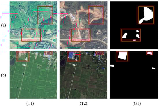
Figure 1. T1 and T2 indicate inconsistencies in imaging conditions that result in style differences in bitemporal images, and red boxes indicate ground object scale differences. Here, T1 is the first temporal-phase, T2 is the second temporal-phase, and GT is the ground truth.

Regarding style differences, existing research has primarily focused on the spatial domain. Most of the methods are feature interaction [20] or feature alignment [21], based on a two-branch multiscale architecture to reduce the domain gap and achieve style unification as much as possible. However, image features in the spatial domain cannot adequately represent image style, resulting in limited effectiveness. Additionally, some researchers have also considered the frequency domain, but they have adopted the same approach as in the spatial domain, performing feature interaction in the frequency domain [22]. While this approach yields a better effect than the spatial domain, it achieves the unification of image styles by constraining the bitemporal features through a shared weight. However, when dealing with bitemporal remote sensing images with significant style differences, its effect is still limited.

To cope with the above challenges, we propose FDFENet. It employs a triple-processing mechanism. First, FFEM transforms images into the frequency domain via a fast Fourier transform (FFT), replacing low-frequency components (encoding illumination and atmosphere) while preserving high-frequency details. This effectively mitigates seasonal and illumination variations, achieving bitemporal image style alignment. In parallel, the FDADM serves as a complementary frequency domain strategy, utilizing dynamic parameter adaptation. Secondly, the MSFEM adopts a two-stage architecture combining a prompt matrix and global enhancement. The prompt matrix serves as a learnable parameter, dynamically enhancing multiscale ground object features through cross-channel interaction with input features. Finally, the MSCPM employs a dual-path attention mechanism to suppress background interference and amplify responses in changing regions, enabling precise localization of subtle changes such as those in cropland.

The main contributions of our work can be summarized as follows:

• Dual Frequency-Domain Solutions for Style Differences: To address style differences, we introduce two frequency domain solutions. The core FFEM replaces low-frequency components to align image styles. In comparison, the FDADM adaptively adjusts parameters to handle style differences. The FFEM emphasizes parameter efficiency and deployment stability, whereas the FDADM emphasizes adaptability and flexibility across different scenarios.
• Collaborative Multiscale Feature Enhancement and Perception: To address the significant scale variations of ground objects, a collaborative mechanism is designed. The MSFEM employs a learnable prompt matrix to dynamically enhance features across scales. The refined features are then processed by the MSCPM, which uses a dual-path attention mechanism to suppress background interference and amplify the response from genuine change areas.
• Effective Hybrid Framework Integrating Diverse Advantages: We propose an effective hybrid framework, FDFENet, which ingeniously integrates the advantages of CNNs (local feature extraction), transformers (global context modeling), attention mechanisms (feature selection), and frequency domain analysis (style alignment). Extensive experiments on four datasets demonstrate that FDFENet outperforms 13 other state-of-the-art methods, validating the effectiveness of this approach.

The rest of this paper is organized as follows. Section 2 briefly reviews the related work. Section 3 describes the specific details of the proposed method. Section 4 presents and analyzes the experimental results. Section 5 discusses the proposed method, and finally, Section 6 summarizes this paper.

2. Related Work

2.1. Deep Learning Architectures for Change Detection

In recent years, numerous deep learning-based CD methods have achieved remarkable results. Among them, approaches based on CNNs and transformers tackle distinct aspects of feature expression. CNNs significantly enhance model performance by deepening backbone networks and optimizing multiscale feature fusion, particularly in complex farmland scenarios. For instance, Zhang et al. [23] introduced a differentiable superpixel segmentation module to suppress pixel-level noise through superpixel constraints. Ma et al. [24] efficiently integrated multiscale features from dual branches and designed a multiscale strip convolutional group for extracting scale-invariant features of continuous objects like water bodies and cropland boundaries and making the edges of the detected objects neater. Although excelling in local feature extraction such as edge and texture representation, CNNs are inherently limited by their local receptive fields, making it difficult to model large-scale spatiotemporal correlations, such as urban sprawl [25] and long-range spatial dependencies in cropland scenes. However, transformers overcome CNNs’ local receptive field limitations by leveraging self-attention to model global dependencies. For example, Chen et al. [26] converted semantic features into semantic tokens and input them into a transformer for global modeling, enlarging the receptive field of the model and realizing a wide range of cropland CD. Liu et al. [27] used a hybrid CNN-Transformer architecture to capture ground object features. Despite these advances, CNN-Transformer-based models struggle to deal with images with large differences in image style, since features in the spatial domain make it difficult to characterize image styles.

2.2. FT for Visual Representation Learning

FFT-based frequency domain analysis for style differences provides a new path for CD. As shown in Figure 1, the frequency domain analysis can largely unify the style differences between images. For example, Chen et al. [28] constructed a frequency-adaptive dilated convolution which dynamically adjusts the expansion rate of the convolution kernel according to the local spectral energy, and it can be used to realize multiscale extraction of farmland boundaries and plot contours. Huang et al. [29] proposed a frequency domain decomposition generalization framework to retain low-frequency structural features such as the appearance of cropland and perturb high-frequency texture noise to enhance cross-domain robustness. In the field of CD, Chen et al. [22] employed the FFT to adaptively filter bitemporal features in the frequency domain while mining the frequency components relevant to cropland change. Zheng et al. [30] focused on the spectral mutations at the edges of buildings via high-frequency attention to improve the accuracy of urban CD, and Guo et al. [31] employed adaptive frequency domain processing and multiscale feature fusion to improve feature extraction in scenarios such as cropland-to-construction land conversion, demonstrating robustness to texture diversity. The above methods have proved the effectiveness of frequency domain analysis, but existing research mainly uses frequency domain analysis to solve other problems, such as boundary contour and feature extraction, and existing research employing frequency domain analysis to process stylistic differences in images remains scarce. Usually, filtering frequency components is used to unify the style in the early stage of the model. However, this method only achieves this by simultaneously enhancing or suppressing the frequency components of bitemporal image features, with a limited effect. Moreover, this method is similar to the attention mechanism and can lead to the premature loss of feature information.

3. Methodology

In this section, we first present an overview of the proposed method. Then, we give the details of the proposed FFEM, MSFEM, and MSCPM. Finally, we will discuss the loss function we used.

3.1. Overall Structure of the Proposed Network

As shown in Figure 2, the FDFENet algorithm consists of four components. (1) The first five layers of ResNet-50 [32] are used as the backbone network. (2) The FFEM performs cross-temporal-phase low-frequency component replacement. (3) The MSFEM and MSCPM first enhance the features of multiscale ground objects by modeling multiscale features and then implement channel-spatial attention to suppress irrelevant information between different temporal phases, thereby refining ground object features. (4) A cascaded classifier is used to achieve multi-level supervision.

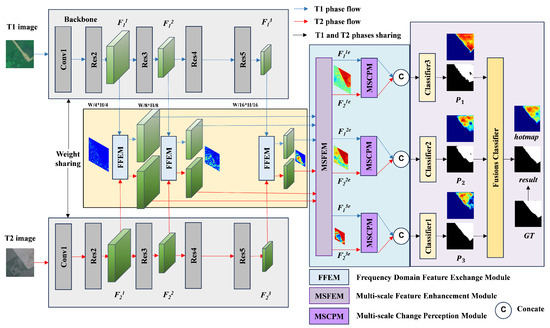
Figure 2. Overall structure diagram of FDFENet. The model uses the FFEM to replace low-frequency features with bitemporal features to unify image styles. It then uses the MSFEM to enhance multiscale features followed by the MSCPM to emphasize multiscale variation information. Finally, the features are input into a multi-level classifier to output the prediction results. All figures have consistent legends.

The FDFENet algorithm uses a dual-stream backbone network to extract three-scale features $F_i^j(i\in \{1,2\},j\in \{1,2,3\})\in {\mathbb{R}}^{C\times H\times W}$ from bitemporal images $\{T_1,T_2\}\in {\mathbb{R}}^{3\times H\times W}$. First, the same-scale features are subjected to an FFT, followed by swapping the low-frequency components and then inverse transform reconstruction to achieve frequency feature alignment. Then, the cross-temporal same-scale aligned features are input into the MSFEM, which integrates local and global information to enhance features. The enhanced features are $F_i^{je}(i\in \{1,2\},j\in \{1,2,3\})\in {\mathbb{R}}^{C\times H\times W}$. Next, the features are optimized through a dual-path attention mechanism (channel attention focuses key semantics channels, and spatial attention focuses on change-sensitive regions). Finally, the enhanced features of the same scale in the two temporal phases are concatenated in the channel dimension and then input into the classifier to obtain the multiscale change maps $P_1,P_2,P_3$. The multiscale classification maps are then integrated into the final change map result (result as the final result) through the fusion classifier.

3.2. Backbone Network

As shown in Figure 2, FDFENet adopts ResNet-50 [32], with the initial fully connected layer removed as the backbone network to extract multiscale features from the input images $T_1\mathrm{and}{T}_2$. The ResNet backbone network consists of five main modules, including a $7\times 7$ convolutional layer and four residual blocks. For the input bitemporal images $\{T_1,T_2\}\in {\mathbb{R}}^{3\times H\times W}$, three-scale features are extracted from ResNet and named $F_i^1,F_i^2,F_i^3,\mathrm{where}i\in \{1,2\}$.

3.3. Dual Frequency-Domain Solutions

Differences in remote sensing image styles stem from varying imaging conditions (e.g, solar elevation angle, atmospheric transmittance, and sensor response), causing missed detection and false detection issues (Figure 1a). We propose two frequency domain mechanisms: (1) the Frequency Domain Feature Exchange Module, which uses an FFT to map features to the frequency domain, swaps low-frequency components in the channel dimension, and achieves zero parameter and zero computational overhead for frecquency feature alignment, and (2) the Frequency Domain Aggregation Distribution Module, which integrates an attention mechanism and dynamically fuses multi-frequency components through learnable weights to establish cross-temporal frequency domain consistency constraints. As shown in Figure 3, this strategy can effectively eliminate pseudo-noise caused by changes in seasonal and lighting factors.

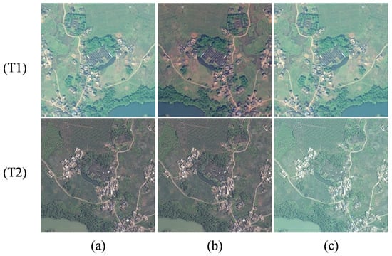
Figure 3. Frequency domain feature exchange for bitemporal images by replacing low-frequency components. This operation correspondingly replaces the colors and brightness of the images. (a) Original bitemporal images. (b) Replacing the low-frequency components of the T1 image with those of the T2 image. (c) Replacing the low-frequency components of the T2 image with those of the T1 image.

3.3.1. Frequency Domain Feature Exchange Module

As shown in Figure 3, the low-frequency components of remote sensing imagery encode global radiometric characteristics [22,29,33], while the high-frequency components carry local structural information [22,34]. Based on this, we propose the FFEM, which performs an FFT [35] on the bitemporal features and achieves cross-temporal feature alignment by replacing the central 1 × 1 low-frequency region. Finally, the IFFT is used for conversion back to the spatial domain to achieve spatial domain feature reconstruction.

The specific process is shown in Figure 4. First, the bitemporal features are subjected to an FFT to convert the features to the frequency domain. To facilitate the exchange of low-frequency components, a centering operation—FFTSHIFT—is used to shift the low-frequency components to the center position. Then, the positions to be exchanged are defined. The position we chose was a square region with a length of 1 at the center of the feature map. Then, using the inverse centralization operation—IFFTSHIFT and IFFT—the features were transformed back to the spatial domain. The bitemporal characteristics are represented by $F_1^j,F_2^j(j\in \{1,2,3\})\in {\mathbb{R}}^{C\times H\times W}$, and the FFT formula is shown in Equation (1):

$$F_{\mathrm{fft},1/2}^j(H,W)=\mathcal{F}\left[F_{1/2}^j(H,W)\right]=\sum _{h=1}^{H-1}\sum _{w=1}^{W-1}{F}_{1/2}^j(H,W)e^{-i2\pi \left({\displaystyle \frac{uh{2}^j}{H}}+{\displaystyle \frac{vw{2}^j}{W}}\right)}$$

(1)

where $F_{\mathrm{fft},1/2}^j\in {\mathbb{R}}^{(H/2^j)\times (W/2^j)\times 2C_j}$ for $j\in \{2,3,4\}$ is the frequency domain feature obtained by applying the FFT to the different resolution features of the $T_1$ phase or $T_2$ phase and i denotes the imaginary unit. The specific process of the FFEM is shown in Equation (2):

$$\begin{array}{c}{f}_1^j,f_2^j=\text{FFT\_SHIFT}\left(\mathrm{FFT}\left(F_1^j\right),\mathrm{FFT}\left(F_2^j\right)\right)\hfill \\ ou{t}_1^j,ou{t}_2^j=\mathrm{IFFT}\left(\text{IFFT\_SHIFT}\left(\mathrm{Exchange}\left(f_1^j,f_2^j\right)\right)\right)\hfill \end{array}$$

(2)

Here, FFI_SHIFT indicates that the centralization operation moves the low-frequency components to the center position. Exchange indicates frequency domain feature exchange. IFFT_SHIFT indicates the inverse centering operation, which restores the low-frequency components after the centering operation to their original positions. FFT indicates the fast fourier transform. Finally, IFFT indicates the inverse fast Fourier transform. The pseudocode for exchange is as shown in Algorithm 1.

Algorithm 1 Frequency Domain Feature Exchange Module

Require: Input features: $F_1^j,F_2^j$ Ensure: Output features after exchange: $ou{t}_1^j,ou{t}_2^j$ 1: Step 1: Translation to frequency domain (shifts low-frequency features to center) 2: $t_1^j,t_2^j\leftarrow \mathrm{FFT}\left(F_1^j\right),\mathrm{FFT}\left(F_2^j\right)$ 3: $f_1^j,f_2^j\leftarrow \text{FFT\_SHIFT}\left(t_1^j\right),\text{FFT\_SHIFT}\left(t_2^j\right)$ 4: Step 2: Frequency domain feature exchange 5: $roi\_h\leftarrow \left({\displaystyle \frac{H}{2}}-changelength:{\displaystyle \frac{H}{2}}+changelength\right)$ 6: $roi\_w\leftarrow \left({\displaystyle \frac{W}{2}}-changelength:{\displaystyle \frac{W}{2}}+changelength\right)$ 7: $temp\leftarrow f_1^j[:,c,roi\_h,roi\_w]$ 8: $f_1^j[:,c,roi\_h,roi\_w]\leftarrow f_2^j[:,c,roi\_h,roi\_w]$ 9: $f_2^j[:,c,roi\_h,roi\_w]\leftarrow temp$ 10: Step 3: Transformation back to space domain 11: $ou{t}_1^j,ou{t}_2^j\leftarrow F_1^j,F_2^j$ 12: $ou{t}_1^j[:,c]\leftarrow \mathrm{IFFT}\left(\text{IFFT\_SHIFT}\left(f_1^j[:,c]\right)\right)$ 13: $ou{t}_2^j[:,c]\leftarrow \mathrm{IFFT}\left(\text{IFFT\_SHIFT}\left(f_2^j[:,c]\right)\right)$ 14: return $ou{t}_1^j,ou{t}_2^j$

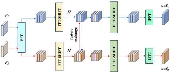
Figure 4. Detailed structure diagram of the FFEM. The module converts images to the frequency domain through an FFT and then exchanges low-frequency features to unify the styles of bitemporal images.

3.3.2. Frequency Domain Aggregation Distribution Module

We propose a Frequency Domain Aggregation Distribution Module (FDADM), shown in Figure 5), whose technical framework integrates the attention mechanism with the principle of frequency domain feature interaction [20,36] to achieve dynamic calibration across temporal-phase features. First, we use an FFT on bitemporal features to obtain frequency domain representations and then construct global collaborative features through frequency domain summation. Next, we use a multi-layer perceptron to decouple frequency domain attention weights from the collaborative features. Finally, we perform feature recalibration and implement channel-adaptive feature enhancement in the frequency domain.

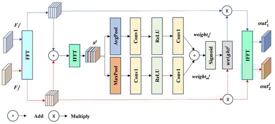
Figure 5. Detailed structure diagram of the FDADM. The module performs feature interaction on bitemporal features in the frequency domain to mitigate style differences between bitemporal images.

This mechanism dynamically adjusts feature responses through frequency domain attention, emphasizing the expression of features in high-frequency sensitive areas such as occupation of cropland and building expansion while suppressing style differences caused by inconsistent imaging conditions, such as cloud cover and shadow movement. The bitemporal features are $F_1^j,F_2^j(j\in \{1,2,3\})\in {\mathbb{R}}^{C\times H\times W}$. The formulas for the FDADM are shown in Equations (3) and (4):

$$\begin{array}{cc}\hfill & s^j=\mathrm{IFFT}\left(\mathrm{FFT}\left(F_1^j\right)+\mathrm{FFT}\left(F_2^j\right)\right)\hfill \\ \hfill & weigh{t}_a^j=\text{Conv1}\left(\mathrm{ReLU}\left(\text{Conv1}\left(\mathrm{Avgpool}\left(s^j\right)\right)\right)\right)\hfill \\ \hfill & weigh{t}_m^j=\text{Conv1}\left(\mathrm{ReLU}\left(\text{Conv1}\left(\mathrm{Maxpool}\left(s^j\right)\right)\right)\right)\hfill \end{array}$$

(3)

$$\begin{array}{c}weigh{t}^j=\mathrm{Sigmoid}\left(weigh{t}_a^j+weigh{t}_m^j\right)\hfill \\ ou{t}_i^j=\mathrm{IFFT}\left(weigh{t}^j·F_i^j\right)(i\in \{1,2\})\hfill \end{array}$$

(4)

Here, AvgPool indicates an average pooling operation. MaxPool indicates a max pooling operation. ReLU and Sigmoid indicate the activation function, Conv1 indicates a convolution operation with a convolution kernel of 1, FFT indicates a fast Fourier transform, and IFFT indicates an inverse fast Fourier transform.

3.4. Multiscale Feature Enhancement Module

The large scale difference of ground objects in remote sensing images is mainly reflected in two aspects. First, within single-phase images, there are significant differences in the scale of cropland of varying sizes. Second, significant scale differences exist between existing cropland and illegally occupied cropland when comparing bitemporal images. This scale disparity can cause feature overlap in traditional single-scale models. Consequently, these models often fail to detect small-scale changes, such as newly constructed small residential buildings and road expansions, resulting in scattered occupation of cropland. This poses a significant challenge to the model’s ability to accurately identify changes in cropland. Therefore, we designed the MSFEM to solve this problem.

As shown in Figure 6, the MSFEM adopts a two-stage architecture of “prompt matrix-global enhancement”. First, a learnable matrix ($p_j(j\in \{1,2,3\})$) is initialized (using a random distribution to facilitate optimization) and then updated during training to capture dataset-specific statistics. This $p_j$ matrix dynamically enhances multiscale ground object features. After channel attention filtering, the feature prompt matrix $promp{t}_i^j(i\in \{1,2\},j\in \{1,2,3\})$ is generated. Then, in the global feature enhancement stage, the original features $ou{t}_i^j$ are concatenated with $promp{t}_i^j$ along the channel dimension and input into the transformer for global modeling.

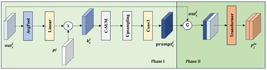
Figure 6. Detailed structure diagram of the MSFEM. The module models multiscale features to enhance the characteristics of multiscale ground objects, thereby improving the model’s ability to recognize multiscale ground objects. Linear indicates a fully connected layer, $p^j$ indicates a randomly generated tensor constant, C-SUM indicates a summation of the channel dimensions, and $promp{t}_i^j$ indicates the feature prompt matrix.

Feature prompt matrices serve as learnable parameter matrices, achieving dynamic enhancement through cross-channel interaction with input features. After concatenation with the feature matrix, the prompt matrix undergoes global modeling via the transformer, thereby playing a prompting role in enhancing the feature of $ou{t}_i^j$. The bitemporal feature is $ou{t}_i^j(i\in \{1,2\},j\in \{1,2,3\})\in {\mathbb{R}}^{C\times H\times W}$. The main MSFEM formulas are shown in Equations (5) and (6):

Phase I:

$$\begin{array}{c}{k}_i^j={\mathrm{p}}^{\mathrm{j}}·\left(\mathrm{Linear}\left(\mathrm{Avgpool}\left(ou{t}_i^j\right)\right)\right)\hfill \\ promp{t}_i^j=\text{Conv3}\left(\mathrm{Upsampling}\left(\text{C-SUM}\left(k_i^j\right)\right)\right)\hfill \end{array}$$

(5)

Phase II:

$${\displaystyle F_i^{je}=\mathrm{Transformer}\left(\mathrm{Cat}\left(promp{t}_i^j,ou{t}_i^j\right)\right)}$$

(6)

Here, Avgpool indicates global average pooling, Linear indicates a fully connected layer, Softmax indicates the normalization function, prompt indicates a randomly generated tensor constant, C-SUM indicates a summation of the channel dimensions, Upsampling indicates an upsampling operation, Conv3 indicates a convolution operation with a $3\times 3$ convolution kernel, and Cat indicates a channel concatenation operation.

The second stage of the MSFEM (global enhancement stage) uses the Transformer module for feature modeling. The transformer is divided into two parts: the encoder and the decoder. First, self-attention is used to encode the features of the first stage’s input. The self-attention mechanism calculates the dot product of the query, key, and value matrices to generate attention scores, which are then normalized using the softmax function to ultimately generate attention weights. The core formula is shown in Equation (7):

$$att=\mathrm{SA}(q,k,v)=\mathrm{Softmax}\left({\displaystyle \frac{q·k^{\top }}{\sqrt{d_k}}}\right)·v$$

(7)

where $d_k$ is the number of columns in k and Softmax indicates the normalization function.

The decoder employs cross-attention to model the dependencies between two distinct feature sets. In the context of change detection (CD) for remote sensing images, cross-attention computes the attention scores between the decoder’s features (queries) and the encoder-derived features (keys and values). These scores are normalized into attention weights, which are then used to compute a weighted sum of the encoder features, thereby producing global feature representations. The formula is consistent with the self-attention mechanism shown in Equation (7).

3.5. Multiscale Change Perception Module

To address the issue of coupling significant and insignificant features in multiscale enhanced features—where enhanced multiscale features contain a large amount of redundant information—we designed the MSCPM, whose core architecture is shown in Figure 7. The MSCPM employs a cross-scale parameter sharing mechanism, generating a global modulation vector through a gated, fully connected network. This vector acts on the features of each scale to suppress the information irrelevant to the change while maintaining the consistency of the features across time and scales. The module consists of a spatially aware unit and a channel-aware unit, both of which utilize a dual-path attention mechanism for feature selection.

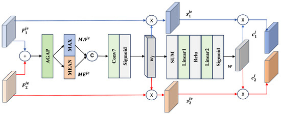
Figure 7. Detailed structure diagram of the MSCPM. The module utilizes dual-path attention to emphasize features related to changes, enhancing the network’s ability to perceive multiscale changes in ground objects. AGAP indicates the adaptive global average pooling operation, MAX indicates the maximum value operation in the channel dimension, MEAN indicates the average operation in the channel dimension, SUM indicates the sum operation, and Linear1 and Linear2 indicate fully connected layers.

The spatial perception unit adopts a cross-temporal feature fusion strategy, capturing common patterns between temporal phases by summing elements of bitemporal features of the same scale. Then, a $3\times 3$ convolution layer and Sigmoid activation are used to generate a spatial attention map to quantify the significance of each pixel area. Finally, the attention weights are synchronously applied to the original bitemporal features, suppressing useless information and maintaining scale consistency. $F_i^{je}(i\in \{1,2\},j\in \{1,2,3\})$ denotes bitemporal features from the same scale but with different temporal phases. The core formulas are shown in Equations (8)–(10):

$$\begin{array}{cc}\hfill & M{A}^{je}=\mathrm{MAX}\left(AGAP(F_1^{je}+F_2^{je})\right),M{E}^{je}=\mathrm{MEAN}\left(AGAP(F_1^{je}+F_2^{je})\right)\hfill \end{array}$$

(8)

$$\begin{array}{cc}\hfill & w^j=\mathrm{Sigmoid}\left(\text{Conv7}\left(\mathrm{Cat}\left(M{A}^{je},M{E}^{je}\right)\right)\right)\hfill \end{array}$$

(9)

$$s_i^j=w^j·F_i^{je}$$

(10)

By adopting a channel compression-stimulation mechanism, the channel perception unit dynamically models the channel response distribution of multi-temporal features through global average pooling. It combines this with a gated, fully connected layer to generate adaptive weights. This design establishes consistency constraints across temporal phases in the channel dimension, effectively suppressing features unrelated to changes and achieving alignment optimization of multi-temporal features. The core formulas are shown in Equations (11) and (12):

$$w=\mathrm{Sigmoid}\left(\text{Linear2}\left(\mathrm{ReLU}\left(\text{Linear1}(\sum _{j=1}^3{w}^j\right)\right)\right)$$

(11)

$$c_i^j=w·s_i^j$$

(12)

Here, AGAP indicates the adaptive global average pooling operation, MAX indicates the maximum value operation in the channel dimension, MEAN indicates the average operation in the channel dimension, Cat indicates the channel concatenation operation, Conv7 indicates the convolution operation with a seven-element convolution kernel, Sigmoid indicates a normalized activation function, Linear1 and Linear2 indicate fully connected layers, and ReLU indicates the activation function.

3.6. Loss Function

The multiscale feature fusion decoder we constructed (Figure 2) consists of a three-stage processing flow. First, cross-branch feature aggregation is used to concatenate the same-scale features of the twin networks along the channel dimension, followed by bilinear interpolation to restore the original resolution. Then, parallel, fully convolutional classifiers are employed to generate three-scale change probability maps $P_1,P_2$, and $P_3$. Finally, the three-scale probability maps are stacked along the channel dimension and input into a cascaded fusion classifier for spatial-semantic collaborative optimization, producing a pixel-level fine-grained CD map result. The model’s loss function is based on the cross-entropy [37] (CE) function, which is defined as follows in Equations (13) and (14):

$${\mathrm{L}}_{\mathrm{ce}}(\mathrm{P},\mathrm{Y})=-{\displaystyle \frac{1}{h_0+w_0}}\sum _{i,j}{Y}_{i,j}\log p_{i,j}$$

(13)

$$\mathrm{Loss}={\mathrm{L}}_{\mathrm{ce}}(P_1,Y)+{\mathrm{L}}_{\mathrm{ce}}(P_2,Y)+{\mathrm{L}}_{\mathrm{ce}}(P_3,Y)+{\mathrm{L}}_{\mathrm{ce}}(result,Y)$$

(14)

We used the cross-entropy loss function for calculating the loss between the predicted images and the label Y, where $h_0$ and $w_0$ are the height and width of the bitemporal images, respectively, and $p_{i,j}$ represents the pixel prediction probability generated by the model.

4. Experiment and Results

In this section, we first discuss the four CD datasets used in the experiments. Next, we introduce the metrics and related experimental details. Then, we quantitatively and qualitatively present the experimental comparison results between FDFENet, its variants, and 13 state-of-the-art methods. Finally, we present the ablation experiment results for FDFENet. All metrics are reported as percentages (%).

4.1. Datasets

CLCD [27]: This high-resolution cropland change detection dataset contains 600 pairs of cropland images, namely $512\times 512$-pixel bitemporal remote sensing images covering two consecutive crop cycles in Guangdong Province, China from 2017 to 2019. The images have a spatial resolution of 0.5–2 m, fully presenting the morphological characteristics of farmland plots and surface coverage details. They are divided into a training set (360 pairs), a validation set (120 pairs), and a test set (120 pairs) at a 6:2:2 ratio.

GFSWCLCD [38]: This dataset is specifically designed to detect complex changes in cultivated land. It contains 1144 pairs of cropland images ($256\times 256$ pixels, 1 m resolution) sourced from Gaofen-2 satellite data. The imagery covers Xinjiang’s Tacheng region during 2018–2023. Covering diverse geographical environments such as plains and lakes, the dataset focuses on depicting detailed patterns of agricultural land expansion and abandonment. It is divided into a training set (687 pairs), validation set (229 pairs), and test set (228 pairs) at a 6:2:2 ratio. This dataset was created by our laboratory and is now open source (http://47.105.192.200/download/showdownload.php?id=29 (accessed on 26 July 2025)).

LuojiaSETCLCD [39]: The mixed-scene dataset, derived from GF-1 and GF-2 satellite imagery, encompasses 4194 bitemporal image pairs ($512\times 512$ pixels) with a 1–2 m spatial resolution. The data span from 2016 to 2018, covering diverse landscape types including urban areas, plains, cropland, and mountainous regions. One defining feature is its highly fragmented agricultural landscape, where farmlands are intricately intertwined with rural settlements, roads, and woodlands, posing significant challenges for boundary precision. The dataset is partitioned into training (2933 pairs), validation (419 pairs), and test (842 pairs) sets at a ratio of 7:1:2.

HRCUSCD [37]: This is a high-resolution urban scene dataset comprising 11,388 pairs of 0.5 m resolution, $256\times 256$-pixel images, spanning a timeframe of long-term (2010–2018) and short-term (2019–2022) dynamic monitoring. It innovatively defines “explicit changes” (new construction or demolition of buildings) and “implicit changes” (unfinished structures), covering six heterogeneous scenarios such as urban villages and industrial parks. The dataset is divided into a training set (7974 pairs), a validation set (2276 pairs), and a test set (1138 pairs) with interference controls, following a 7:2:1 ratio. Although HRCUSCD is primarily an urban dataset, we included it to evaluate the model’s performance in detecting construction activities. This is intended to simulate the detection of cropland non-agriculturalization (e.g., cropland being occupied by buildings), which requires the model to accurately identify artificial targets.

4.2. Evaluation Metrics

To validate the performance of the proposed network, we used five metrics to evaluate the similarity between the predicted results and the actual changes, including the precision (Pre), recall (Rec), F1 score (F1), intersection over union (IOU), and overall accuracy (OA). Each metric can be defined as follows:

$$\mathrm{Pre}={\displaystyle \frac{\mathrm{TP}}{\mathrm{TP}+\mathrm{FP}}}$$

(15)

$$\mathrm{Rec}={\displaystyle \frac{\mathrm{TP}}{\mathrm{TP}+\mathrm{FN}}}$$

(16)

$$\mathrm{F}1={\displaystyle \frac{2·\mathrm{Pre}·\mathrm{Rec}}{\mathrm{Pre}+\mathrm{Rec}}}$$

(17)

$$\mathrm{IOU}={\displaystyle \frac{\mathrm{TP}}{\mathrm{TP}+\mathrm{FP}+\mathrm{FN}}}$$

(18)

$$\mathrm{OA}={\displaystyle \frac{\mathrm{TP}+\mathrm{TN}}{\mathrm{TP}+\mathrm{TN}+\mathrm{FP}+\mathrm{FN}}}$$

(19)

Among these equations, TP, FP, TN, and FN represent the number of true positives, false positives, true negatives, and false negatives, respectively.

4.3. Implementation Details

The experiment was implemented using the PyTorch 1.12.0 framework and trained on a single NVIDIA A40 GPU (48 GB, CUDA 12.1). Parameter updates employed the AdamW [40] optimizer (base learning rate of 0.0001, weight decay of 0.01) with a maximum training epoch of 100. Batch sizes were dynamically allocated based on the dataset characteristics (CLCD, GFSWCLCD, and LuojiaSETCLCD were 8, and HRCUSCD was 32). The model employed a pretrained ResNet-50 backbone on ImageNet, with the transformer module utilizing a common Transformer architecture (we used only one encoder and one decoder) configured as follows: token_len = 4, depth = 1, and heads = 8. The training strategies included data augmentation (random rotation of 0–180° and multi-directional flipping), a dynamic learning rate (decreased by 0.95 when the validation set’s IOU failed to improve for 6 consecutive epochs, capped at 3 reductions), and early stopping (termination if the IOU remained unchanged after 3 learning rate reductions and 6 epochs). Mixed-precision training optimizes GPU memory utilization. Data augmentation was disabled during testing, directly outputting the CD map from the fusion classifier to ensure result reproducibility.

4.4. Comparison with the State-of-the-Art Methods

We compared the proposed method with a series of state-of-the-art bitemporal CD networks, including convolutional neural network-based networks (HCGMNet), attention mechanism-based networks (AMT-Net, B2CNet, FMCD, GAS, CACD, and CGNet), networks based on both convolutional neural networks and attention mechanisms (SGSLN, ELGCNet, and HSANet), and networks based on transformers (BIT, MSCANet, and STMTNet):

• HCGMNet [41]: A layered convolutional guidance network is used, employing a multi-scale feature fusion strategy and a change guidance module to enhance edge feature expression capabilities.
• AMTNet [8]: A twin network model that combines CNN, multiscale, Transformer, and attention mechanisms to effectively detect changes by maximizing the advantages of various methods.
• B2Net [42]: A boundary-oriented network builds a progressive optimization mechanism from the boundary to the center, using a boundary sensing module to suppress feature noise interference.
• FMCD [21]: This multi-level feature interaction framework combines a multi-task learning paradigm and mixed attention mechanism to strengthen inter-temporal feature correlation modeling.
• GASNet [43]: A global-local perception network establishes dynamic associations between the scene context and foreground objects, improving object recognition capabilities in complex backgrounds.
• CACDNet [44]: This cascaded dual decoder architecture achieves boundary refinement optimization from coarse-grained to fine-grained through hierarchical feature integration.
• CGNet [45]: Self-attention driven networks generate semantic prior information through variation guidance modules and combine long-range dependency modeling to optimize multi-scale feature fusion.
• SGSLN [46]: This dual-path feature interaction architecture utilizes semantic fusion strategies at the decision layer to resolve ambiguity issues in multi-encoder feature inference.
• ELGCNet [47]: An efficient global and local context aggregation network was proposed that utilizes rich contextual information to accurately estimate change regions while reducing model parameters.
• HSANet [48]: This hybrid attention network integrates self-attention and cross-attention mechanisms to achieve cross-scale global context modeling and edge detail enhancement.
• BIT [26]: This represents images as semantic tokens and performs spatiotemporal context modeling on semantic tokens using transformers.
• MSCANet [27]: This multi-scale encoding and decoding network combines CNN local feature extraction and Transformer global modeling capabilities, optimizing cross-layer feature aggregation.
• STMTNet [49]: This dual-stream triad network integrates FastSAM and VGGNet16 for geometric-semantic analysis via spatiotemporal gating and multiscale enhancement, suppresses seasonal noise, and refines fragmented boundaries.

For each dataset, we used official (if available) or commonly used unofficial codes, while all comparison data adopted our locally reproduced results. For all experiments, if no significant annotation was provided, then ResNet50 was used as the backbone network by default. The method using the FFEM was named FDFENet(FFE_R50), abbreviated as FFE_R50, and the method using the FDADM was named FDFENet(AD_R50), abbreviated as AD_R50.

4.4.1. Experimental Results on CLCD Dataset

As shown in Table 1, our FFE_R50 method significantly outperformed all comparison methods on the CLCD dataset in terms of Pre, F1, IOU, and OA. Specifically, FFE_R50 achieved improvements of 3.73%, 1.25%, 1.63%, and 0.35% over the third-highest method in terms of Pre, F1, IOU, and OA, respectively. Meanwhile, the AD_R50 method achieved the second-best performance for Pre and OA and the third-highest performance for F1 and IOU. Specifically, AD_R50 saw increases of 0.63% and 0.1%, respectively, compared with the third-highest Pre and OA values. Overall, although FFE_R50 did not have the highest Rec, its overall performance was more balanced, and it maintained the best performance in the core metrics of F1 and IOU.

Table 1. Performance comparison of different CD methods on the CLCD dataset. The best results are highlighted in red, the second-best results are highlighted in green, and the third-best results are highlighted in blue.

Methods	Pre (%)	Rec (%)	F1 (%)	IOU (%)	OA (%)
HCGMNet [41]	68.81	74.70	71.63	55.80	95.72
AMTNet [8]	77.14	73.27	75.15	60.02	96.40
B2Net [42]	65.48	78.80	71.53	55.67	95.33
FMCD [21]	77.35	71.90	74.53	59.40	96.34
GASNet [43]	63.17	75.51	68.79	52.42	94.90
CACDNet [44]	71.91	81.09	76.23	61.58	96.24
CGNet [45]	69.52	73.13	71.28	55.37	95.74
SGSLN [46]	69.94	68.38	69.15	52.85	95.46
ELGCNet [47]	71.20	61.12	65.78	49.00	95.27
HSANet [48]	70.87	71.51	71.19	55.26	95.69
BIT [26]	61.72	62.23	61.97	44.90	94.32
MSCANet [27]	74.11	66.64	70.18	54.06	95.79
STMTNet [49]	69.79	78.57	73.92	58.63	95.85
FDFENet(AD_R50)	77.98	73.82	75.84	61.09	96.50
FDFENet(FFE_R50)	81.08	73.47	77.09	62.72	96.75

4.4.2. Experimental Results on GFSWCLCD Dataset

As shown in Table 2, our FFE_R50 method achieved significantly better Rec results than all comparison methods on the GFSWCLCD dataset, and it achieved the second-best results for OA, F1, and IOU. Specifically, FFE_R50 achieved improvements of 1.43%, 0.71%, 1.06%, and 0.04% over the third-highest method in terms of Rec, F1, IOU, and OA, respectively. Meanwhile, the AD_R50 method achieved the best performance for Pre, F1, IOU, and OA and the third-highest performance for Rec. Specifically, AD_R50 saw increases of 0.76%, 0.98%, 1.47%, and 0.4% compared with the third-highest values for Pre, F1, IOU, and OA, respectively. The performance gap between the two models on GFSWCLCD was minimal (F1 difference of 0.27% and IOU difference of 0.41%). Given the stability advantage of the FFEM’s zero parameter count, the FFEM is recommended.

Table 2. Performance comparison of different CD methods on the GFSWCLCD dataset. The best results are highlighted in red, the second-best results are highlighted in green, and the third-best results are highlighted in blue.

Methods	Pre (%)	Rec (%)	F1 (%)	IOU (%)	OA (%)
HCGMNet [41]	80.52	83.77	82.11	69.65	90.33
AMTNet [8]	82.38	83.00	82.69	70.49	90.79
B2Net [42]	80.30	83.50	81.87	69.30	90.20
FMCD [21]	79.87	83.88	81.83	69.24	90.13
GASNet [43]	81.35	83.80	82.55	70.29	90.62
CACDNet [44]	84.26	80.44	82.31	69.94	90.74
CGNet [45]	83.58	82.13	82.85	70.71	90.99
SGSLN [46]	79.69	85.27	82.39	70.05	90.34
ELGCNet [47]	83.26	76.40	79.68	66.22	89.68
HSANet [48]	82.76	83.09	82.92	70.83	90.93
BIT [26]	83.07	76.94	79.89	66.51	89.73
MSCANet [27]	80.83	82.26	81.54	68.83	90.30
STMTNet [49]	84.24	83.42	83.83	72.16	91.57
FDFENet(AD_R50)	85.00	84.63	84.81	73.63	91.97
FDFENet(FFE_R50)	83.07	86.06	84.54	73.22	91.66

4.4.3. Experimental Results on LuojiaSETCLCD Dataset

As shown in Table 3, our FFE_R50 method achieved the second-best results in terms of F1 and IOU on the LuojiaSETCLCD dataset. Specifically, FFE_R50 improved these metrics by 0.05% and 0.06% over the third-highest results for F1 and IOU, respectively. Meanwhile, the AD_R50 method achieved the best results in terms of F1 and IOU and the third-highest results in terms of OA. Compared with the third-highest results, the AD_R50 method improved the F1 and IOU by 0.29% and 0.36%, respectively. The performance difference between FFE_R50 and AD_R50 was minimal (0.24% difference in F1 and 0.30% difference in IOU). Since the FDADM requires learning parameters, leading to insufficient stability, the zero-parameter FFEM scheme is recommended.

Table 3. Performance comparison of different CD methods on the LuojiaSETCLCD dataset. The best results are highlighted in red, the second-best results are highlighted in green, and the third-best results are highlighted in blue.

Methods	Pre (%)	Rec (%)	F1 (%)	IOU (%)	OA (%)
HCGMNet [41]	75.16	71.06	73.52	58.13	98.34
AMTNet [8]	73.24	71.50	72.36	56.69	98.17
B2Net [42]	60.66	86.23	71.22	55.30	97.66
FMCD [21]	72.90	75.33	74.09	58.85	98.23
GASNet [43]	67.87	77.49	72.36	56.70	98.01
CACDNet [44]	70.13	78.03	73.87	58.57	98.15
CGNet [45]	75.66	71.28	73.40	57.98	98.32
SGSLN [46]	74.21	74.15	74.18	58.96	98.27
ELGCNet [47]	72.65	68.67	70.60	54.56	98.08
HSANet [48]	72.52	74.43	73.46	58.05	98.26
BIT [26]	71.97	74.74	71.97	56.22	98.18
MSCANet [27]	67.78	72.22	69.93	53.76	97.91
STMTNet [49]	70.44	69.76	70.10	53.96	98.23
FDFENet(AD_R50)	74.19	74.75	74.47	59.32	98.28
FDFENet(FFE_R50)	74.02	74.43	74.23	59.02	98.26

4.4.4. Experimental Results on HRCUSCD Dataset

As shown in Table 4, our FFE_R50 method achieved the best results on the HRCUSCD dataset in terms of Pre, F1, IOU, and OA. Specifically, FFE_R50 showed improvements of 0.54%, 2.25%, 2.88%, and 0.08% over the third-highest results in terms of Pre, F1, IOU, and OA, respectively. Meanwhile, the AD_R50 method achieved the second-best results for F1, IOU, and OA and the third-highest Pre. Compared with the third-highest results, the method improved by 1.57%, 1.99%, and 0.04% the F1, IOU, and OA values, respectively. FFE_R50 significantly outperformed the baseline model, with the F1 and IOU core metrics leading the third-highest results by 2.25% and 2.88%, respectively, validating the superiority of our approach.

Table 4. Performance comparison of different CD methods on the HRCUSCD dataset. The best results are highlighted in red, the second-best results are highlighted in green, and the third-best results are highlighted in blue.

Methods	Pre (%)	Rec (%)	F1 (%)	IOU (%)	OA (%)
HCGMNet [41]	75.25	67.02	70.90	54.91	98.97
AMTNet [8]	74.60	71.20	72.86	57.31	99.01
B2Net [42]	37.09	91.15	52.72	35.80	96.94
FMCD [21]	77.17	70.52	73.70	58.35	99.06
GASNet [43]	60.03	81.83	69.26	52.97	98.64
CACDNet [44]	49.42	88.86	63.52	46.54	98.08
CGNet [45]	78.91	66.09	71.93	56.17	99.03
SGSLN [46]	74.06	64.67	69.05	52.73	98.91
ELGCNet [47]	66.94	62.81	64.81	47.94	98.72
HSANet [48]	75.50	64.23	69.41	53.15	98.94
BIT [26]	67.84	72.09	69.90	53.73	98.84
MSCANet [27]	75.40	66.18	70.49	54.43	98.96
STMTNet [49]	76.08	67.28	71.41	55.53	98.99
FDFENet(AD_R50)	77.60	73.07	75.27	60.34	99.10
FDFENet(FFE_R50)	79.45	72.75	75.95	61.23	99.14

In summary, on the CLCD dataset with pronounced stylistic variations, the parameter-free FFEM significantly outperformed the FDADM (F1: 77.09% vs. 75.84%, a gap of 1.25%), demonstrating that the FFEM’s direct low-frequency replacement strategy exhibited greater robustness and effectiveness in unifying image styles. However, in complex scenes with less pronounced style differences, the FFEM and FDADM exhibited comparable performance with minimal variation. On GFSWCLCD and LuojiaSETCLCD, the FDADM held a slight advantage due to its adaptability (F1 score gaps of only 0.27% and 0.24%, respectively). On HRCUSCD, the FFEM regained a slight lead (F1 gap of 0.68%). Although the FDADM exhibited negligible marginal advantages (<0.3%) under subtle style variations, it introduced additional learning parameters and potential instability. In contrast, the FFEM achieved stable performance across all datasets without introducing any extra parameters. Therefore, considering stability, cross-style generalization, and engineering deployment, we explicitly recommend the FFEM as the primary solution. However, the advantage of the FDADM lies in its adaptability and flexibility, which stem from its parameters. For images with subtle stylistic differences, and assuming parameter complexity and stability are not the primary constraints, we suggest using the FDADM.

4.5. Visual Comparison

As shown in (Figure 8, Figure 9, Figure 10 and Figure 11), this study conducted multi-dimensional visualization comparison experiments on four datasets (CLCD, GFSWCLCD, LuojiaSETCLCD, and HRCUSCD) for different-scale ground objects and scene style differences. Five typical sample groups were selected (the first three groups consisting of small-scale ground objects and the last two groups consisting of large-scale ground objects). Visualization of style differences was demonstrated on both CLCD and LuojiaSETCLCD, where better results corresponded to fewer red and green pixels. To achieve a more intuitive visualization, we selected five representative methods from the comparison approach for display. From left to right are images1, images2, and Ground Truth. followed by the results of various models, including HCGMNet, AMT_Net, CACDNet, HSANet, STMTNet, AD_R50, and FFE_R50.

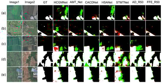
Figure 8. Qualitative results on CLCD. TP = white, TN = black, FP = green, and FN = red. Images1 denotes the first temporal-phase, images2 denotes the second temporal-phase, and GT denotes Ground Truth. HCGMNet, AMT_Net, CACDNet, HSANet, and STMTNet are the names of different comparison methods. AD_R50 and FFE_R50 are abbreviations for FDFENet(AD_R50) and FDFENet(FFE_R50), respectively.

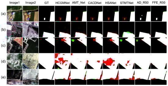
Figure 9. Qualitative results on GFSWCLCD. TP = white, TN = black, FP = green, and FN = red. Images1 denotes the first temporal-phase, images2 denotes the second temporal-phase, and GT denotes Ground Truth. HCGMNet, AMT_Net, CACDNet, HSANet, and STMTNet are the names of different comparison methods. AD_R50 and FFE_R50 are abbreviations for FDFENet(AD_R50) and FDFENet(FFE_R50), respectively.

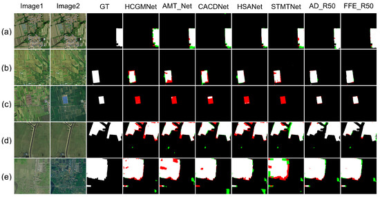
Figure 10. Qualitative results on LuojiaSETCLCD. TP = white, TN = black, FP = green, and FN = red. Images1 denotes the first temporal-phase, images2 denotes the second temporal-phase, and GT denotes Ground Truth. HCGMNet, AMT_Net, CACDNet, HSANet, and STMTNet are the names of different comparison methods. AD_R50 and FFE_R50 are abbreviations for FDFENet(AD_R50) and FDFENet(FFE_R50), respectively.

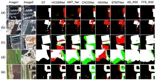
Figure 11. Qualitative results on HRCUSCD. TP = white, TN = black, FP = green, and FN = red. Images1 denotes the first temporal-phase, images2 denotes the second temporal-phase, and GT denotes Ground Truth. HCGMNet, AMT_Net, CACDNet, HSANet, and STMTNet are the names of different comparison methods. AD_R50 and FFE_R50 are abbreviations for FDFENet(AD_R50) and FDFENet(FFE_R50), respectively.

Through a comprehensive analysis of the visualization comparison experiments, in terms of cross-scale detection performance, FFE_R50 and AD_R50 significantly reduced false positives (red areas) and false negatives (green areas) for small-scale targets (such as cropland fragments and unfinished structures) compared with the other methods. For large-scale targets (building clusters and cropland boundaries), the model effectively improved the edge fitting accuracy of the change regions, significantly suppressing fragmented false negatives and false positives in expanded scenarios such as roads, villages, and cities. In terms of style difference, FDFENet significantly reduced both false detection and missed detection rates in both the CLCD and LuojiaSETCLCD style difference samples, which verifies the effectiveness of the frequency domain alignment mechanism. For the AD_R50 method, its performance was similar to that of FFE_R50, but its stability was inferior to that of FFE_R50. For example, in Figure 8b, the results of AD_R50 were not the best compared with other contrast methods. In summary, both the FDADM and FFEM can effectively suppress errors caused by style differences. Through the synergistic effects of frequency domain feature alignment and multi-scale enhancement and perception mechanisms, FDFENet can effectively solve complex problems involving style differences and large differences in ground object scales, providing an innovative perspective for engineering applications under such conditions.

4.6. Ablation Study

In all ablation experiments, we used ResNet-50 as the backbone network of the algorithm to confirm the effectiveness of each key component in the proposed method, and we chose the most dominant indicators (F1 and IOU) for presentation. The symbol “×” indicates that the corresponding module was removed, and “✓” indicates that the corresponding module was used. We used a red font to highlight the best results.

4.6.1. Module Ablation Experiment

To validate the contributions of FDFENet’s components, we conducted a comprehensive ablation study. The experiments were performed on the CLCD, GFSWCLCD, HRCUSCD, and LuojiaSETCLCD datasets, evaluating the independent and synergistic effects of the FFEM, FDADM, MSFEM and MSCPM.

Frequency Domain Feature Exchange Module and Frequency Domain Aggregation Distribution Module

FFEM removal experiment: After removing the FFEM from the FFE_R50 (Table 5), the F1 of the CLCD, GFSWCLCD, HRCUSCD, and LuojiaSETCLCD datasets decreased by 1.79%, 0.90%, 0.99%, and 0.40%, respectively. The corresponding IOU indicators decreased by 2.33%, 1.55%, 1.73%, and 0.84%, respectively.

Table 5. Ablation experiment results of FDFENet (FFE_R50) on the CLCD, GFSWCLCD, HRCUSCD, and LuojiaSETCLCD datasets. The best results are highlighted in red.

FFEM	MSFEM	MSCPM	CLCD		GFSWCLCD		HRCUSCD		LuojiaSETCLCD
			F1 (%)	IOU (%)	F1 (%)	IOU (%)	F1 (%)	IOU (%)	F1 (%)	IOU (%)
×	×	×	72.67	57.86	82.17	70.19	71.65	56.30	71.72	56.13
×	×	✓	73.52	58.13	83.21	71.82	74.41	59.25	72.50	56.86
×	✓	×	73.68	58.70	82.90	70.79	73.30	57.85	73.47	58.32
×	✓	✓	75.30	60.39	83.64	71.67	74.96	59.70	73.83	58.69
✓	×	×	73.87	58.86	83.22	71.27	71.94	56.78	73.05	57.52
✓	×	✓	75.47	60.76	83.88	71.86	74.81	59.50	73.43	58.18
✓	✓	×	75.67	61.05	83.55	71.66	74.88	59.84	73.42	58.01
✓	✓	✓	77.09	62.72	84.54	73.22	75.95	61.23	74.23	59.02

FDADM removal experiment: After removing the FDADM from the AD_R50 (Table 6), the F1 index of the above four datasets decreased by 0.54%, 1.17%, 0.31%, and 0.64%, respectively, and the IOU index decreased by 0.70%, 1.96%, 0.64%, and 0.63%, respectively.

Table 6. Ablation experiment results of FDFENet (AD_R50) on the CLCD, GFSWCLCD, HRCUSCD, and LuojiaSETCLCD datasets. The best results are highlighted in red.

FDADM	MSFEM	MSCPM	CLCD		GFSWCLCD		HRCUSCD		LuojiaSETCLCD
			F1 (%)	IOU (%)	F1 (%)	IOU (%)	F1 (%)	IOU (%)	F1 (%)	IOU (%)
×	×	×	72.67	57.86	82.17	70.19	71.65	56.30	71.72	56.13
×	×	✓	73.52	58.13	83.21	71.82	74.41	59.25	72.50	56.86
×	✓	×	73.68	58.70	82.90	70.79	73.30	57.85	73.47	58.32
×	✓	✓	75.30	60.39	83.64	71.67	74.96	59.70	73.83	58.69
✓	×	×	72.83	57.93	83.74	72.03	73.76	58.43	73.17	57.64
✓	×	✓	74.89	59.86	83.70	71.95	74.27	59.07	73.89	58.59
✓	✓	×	75.71	60.92	83.89	72.58	74.16	58.93	73.96	58.68
✓	✓	✓	75.84	61.09	84.81	73.63	75.27	60.34	74.47	59.32

The effects of the FFEM and FDADM on improving model performance were fully verified. Additionally, the F1 decrease after removing the FFEM on the HRCUSCD dataset was significantly higher than that of the FDADM, further demonstrating that the FFEM shows greater advantages in terms of model performance stability.

Multiscale Feature Enhancement Module and Multiscale Change Perception Module

In the architecture of FDFENet, the MSFEM and MSCPM constitute an “augmentation-aware” cascade for processing structures. This collaborative design solves the two major challenges of feature scale difference and feature enhancement noise.

The MSFEM solves the problem of scale difference in ground objects and dynamically enhances multi-scale ground objects through a learnable cue matrix. As shown in Table 5, the MSFEM was removed from the FFE_R50 model (the MSCPM was retained), and the model performance decreased on all datasets, especially on the CLCD dataset, where the IOU decreased by 1.96%. This proves that the MSFEM plays a key role in solving the problem of missed detection and false detection caused by scale differences. However, the MSFEM inevitably amplified noise while enhancing features. At this point, the synergy of the MSCPM as a “perceptron” is crucial. The dual-path attention mechanism of the MSCPM filters and refines the output features of the MSFEM, suppresses background interference, and amplifies the response of the real change area.

Aside from that, the effectiveness of the MSCPM module was also verified. As shown in Table 5, when removing the MSCPM alone and keeping the MSFEM, the F1 and IOU metrics showed significant decreases on all datasets. On the CLCD dataset, the F1 was reduced by 1.62%, and the IOU was reduced by 1.69%. This loss confirms the irreplaceability of the MSCPM, emphasizing key changes and suppressing redundant information in feature maps.

4.6.2. Model Heat Map Analysis

To validate the interpretability of the module, this study utilized Grad-CAM [40] visualization of the FFI_R50 heat map (Figure 12 and Figure 13). Analysis of the CLCD and GFSWCLCD thermal maps showed that, in terms of scale response, Scale1 primarily activated macro-level targets such as building clusters and large cropland, Scale2 focused on village buildings and medium-sized plot boundaries, and Scale3 exhibited high sensitivity to individual buildings and small cropland fragments. Meanwhile, multi-scale fusion (MIXScale) effectively integrated the prominent areas across all scales. Functionally, the MSFEM enhanced key change features like occupation of cropland and new building construction, although it generated some noise and useless features. Next, the MSCPM suppressed irrelevant features (including useless information enhanced by the MSFEM and seasonal variations) while enhancing cropland boundary and building contour recognition. Notably, the heat map processing pipeline (backbone network→MSFEM→MSCPM) exhibited a progressive optimization characteristic of global perception→multi-scale filtering→change region focus, fully validating the effectiveness of the module’s cascading design.

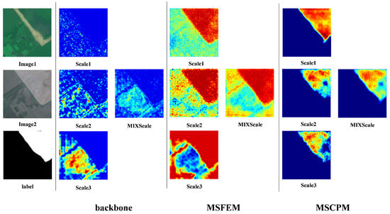
Figure 12. CLCD Grad-CAM visualization results.

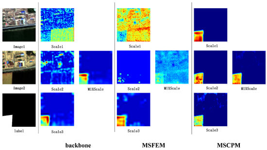
Figure 13. GFSWCLCD Grad-CAM visualization results.

4.6.3. Performance Analysis of Frequency Domain Feature Exchange Module

Feature interaction effectively reduces false detections and missed detections caused by style differences by suppressing the domain gap in bitemporal images. Comparative experiments (Table 7) show that existing spatial domain feature interaction methods (such as SEX [20] channel swapping and SAD [20] shared weight constraints to maintain consistency between bitemporal features) can mitigate the domain gap as much as possible, but their performance was inferior to that of frequency domain methods. The proposed FFEM and FDADM outperformed the spatial domain methods. Specifically, the FFEM achieved the best results on the CLCD and HRCUSCD datasets, while the FDADM achieved the highest F1 and IOU values on the GFSWCLCD and LuojiaSETCLCD datasets. This validates that frequency domain methods are more effective than spatial domain methods in unifying the style of bitemporal images.

Table 7. Comparison results between the FFEM and FDADM and the spatial feature interaction module on the CLCD, GFSWCLCD, LuojiaSETCLCD, and HRCUSCD datasets, with SEX and SAD used in the best way described in the original paper. The best results are highlighted in red.

Module	CLCD		GFSWCLCD		LuojiaSETCLCD		HRCUSCD
	F1 (%)	IOU (%)	F1 (%)	IOU (%)	F1 (%)	IOU (%)	F1 (%)	IOU (%)
SEX	72.71	57.12	84.41	73.03	73.04	57.53	71.72	55.91
SAD	74.69	59.60	83.40	71.53	72.31	56.63	74.29	59.09
FDADM	75.84	61.09	84.81	73.63	74.47	59.32	75.27	60.34
FFEM	77.09	62.72	84.54	73.22	74.23	59.02	75.95	61.23

4.7. Analysis of the Number of Channels Exchanged by the FFEM

When exchanging frequency domain features, what proportion of features should be exchanged? As shown in Table 8, we tried different exchange ratios, ranging from 1/32 to 1. We found that the performance of the FFEM varied relatively little across the four datasets at different exchange ratios. However, a comprehensive analysis of the ablation results indicated that the best performance was achieved at an exchange ratio of 1/2. Therefore, we selected 1/2 as the exchange ratio. For other datasets, the exchange ratio would require experimental evaluation. If no assessment is conducted, then we would recommend 1/2.

Table 8. FFEM ablation study comparison results of channel exchange ratios on the CLCD, GFSWCLCD, LuojiaSETCLCD, and HRCUSCD datasets. The best results are highlighted in red.

Exchange Ratio	CLCD		GFSWCLCD		LuojiaSETCLCD		HRCUSCD
	F1 (%)	IOU (%)	F1 (%)	IOU (%)	F1 (%)	IOU (%)	F1 (%)	IOU (%)
1/1	72.67	57.07	82.73	70.54	72.83	57.27	73.86	58.56
1/2	77.09	62.72	84.54	73.22	74.23	59.02	75.95	61.23
1/4	75.21	60.27	83.90	72.26	73.23	57.77	73.93	58.65
1/8	74.84	59.80	83.72	71.99	73.36	57.93	73.72	58.37
1/16	75.34	60.44	83.61	71.84	72.44	56.79	71.72	55.91
1/32	76.06	61.37	83.75	72.04	73.98	58.70	74.29	59.09

5. Discussion

After introducing the FFEM, MSFEM and MSCPM, compared with the third-highest method in the comparison experiment, this model remained ahead in the core indicators of the F1 and IOU, especially on the HRCUSCD dataset (F1 and IOU were ahead by 2.25% and 2.88%, respectively). Second was GFSWCLCD (1.62% and 2.39%, respectively), while CLCD and LuojiaSETCLCD also had good results. These findings demonstrate that our model is highly effective in addressing style differences and ground object scale differences, and it exhibits strong generalization capability across diverse datasets.

Visual comparisons showed significantly fewer false and missed detections. The small performance gap on LuojiaSETCLCD was likely due to highly fragmented cropland in Wuhan, which poses greater challenges than the larger cropland in Xinjiang. Nevertheless, our model remained robust, demonstrating strong generalization. Ablation experiments confirmed the effectiveness of each module. The FFEM and FDFEM can effectively unify image styles, while the collaboration between the MSFEM and MSCPM also demonstrated exceptional performance when handling scale differences. The heat map reveals the model checking mechanism, and the comparison with the spatial domain module proves the effectiveness and advantages of introducing the frequency domain to solve the style differences.

Finally, it should be noted that the channel exchange ratio of the FFEM needs to be tuned for different data sets, and currently, only the baseline value is provided. In the future, the GFSWCLCD dataset will be extended to provide a more solid database for cropland change detection.

6. Conclusions

FDFENet is an end-to-end cropland change detection framework designed to address image style differences and ground object scale differences. Its core FFEM aligns bitemporal image styles by swapping low-frequency components, with an FDADM provided as a comparative alternative. The system further incorporates the MSFEM to enhance feature representation and the MSCPM to suppress non-change information. These two modules collaborate to improve the model’s detection sensitivity for ground objects at different scales.

Extensive experiments on three public datasets (CLCD, LuojiaSETCLCD, and HRCUSCD) and our newly self-built GFSWCLCD dataset show that FDFENet consistently outperformed 13 state-of-the-art methods, demonstrating its effectiveness in handling style and scale differences. Nevertheless, several limitations remain. First, the FFEM effectively handles pronounced style differences, but its effectiveness diminishes when style differences are not pronounced. Although the FDADM offers adaptability and flexibility, its current design remains confined to image style problems and shows limited effectiveness for other issues. Moreover, all experiments were conducted on RGB imagery, leaving the multispectral and hyperspectral extensions unexplored.

Future work will investigate multi-modal frameworks, adaptive frequency-domain strategies, and the incorporation of long time series data to enhance temporal consistency. Despite current constraints, FDFENet provides a robust foundation for high-precision cropland monitoring, with promising applications in precision agriculture, land degradation assessment, and sustainable cropland use policy development.

References

- Wang, J.; Zhong, Y.; Zhang, L. Change Detection Based on Supervised Contrastive Learning for High-Resolution Remote Sensing Imagery. IEEE Trans. Geosci. Remote Sens. 2023, 61, 1–16. [Google Scholar] [CrossRef]
- Wu, C.; Du, B.; Zhang, L. Fully Convolutional Change Detection Framework with Generative Adversarial Network for Unsupervised, Weakly Supervised and Regional Supervised Change Detection. IEEE Trans. Pattern Anal. Mach. Intell. 2023, 45, 9774–9788. [Google Scholar] [CrossRef]
- Fang, H.; Guo, S.; Wang, X.; Liu, S.; Lin, C.; Du, P. Automatic Urban Scene-Level Binary Change Detection Based on a Novel Sample Selection Approach and Advanced Triplet Neural Network. IEEE Trans. Geosci. Remote Sens. 2023, 61, 1–18. [Google Scholar] [CrossRef]
- Hamidi, E.; Peter, B.G.; Muñoz, D.F.; Moftakhari, H.; Moradkhani, H. Fast Flood Extent Monitoring with SAR Change Detection Using Google Earth Engine. IEEE Trans. Geosci. Remote Sens. 2023, 61, 1–19. [Google Scholar] [CrossRef]
- Luo, S.; Qian, Y.; Bai, L.; Fan, Y.; Wang, Y.; Kong, W. Deep learning-based hyperspectral and multispectral fusion techniques: Review, optimization, and perspectives. Inf. Fusion 2025, 124, 103291. [Google Scholar] [CrossRef]
- Bovolo, F.; Bruzzone, L. A Theoretical Framework for Unsupervised Change Detection Based on Change Vector Analysis in the Polar Domain. IEEE Trans. Geosci. Remote Sens. 2007, 45, 218–236. [Google Scholar] [CrossRef]
- Celik, T. Unsupervised Change Detection in Satellite Images Using Principal Component Analysis and k-Means Clustering. IEEE Geosci. Remote Sens. Lett. 2009, 6, 772–776. [Google Scholar] [CrossRef]
- Liu, W.; Lin, Y.; Liu, W.; Yu, Y.; Li, J. An attention-based multiscale transformer network for remote sensing image change detection. ISPRS J. Photogramm. Remote Sens. 2023, 202, 599–609. [Google Scholar] [CrossRef]
- Xiang, S.; Wang, M.; Jiang, X.; Xie, G.; Zhang, Z.; Tang, P. Dual-task semantic change detection for remote sensing images using the generative change field module. Remote Sens. 2021, 13, 3336. [Google Scholar] [CrossRef]
- Chen, P.; Zhang, B.; Hong, D.; Chen, Z.; Yang, X.; Li, B. FCCDN: Feature constraint network for VHR image change detection. ISPRS J. Photogramm. Remote Sens. 2022, 187, 101–119. [Google Scholar] [CrossRef]
- Miao, L.; Li, X.; Zhou, X.; Yao, L.; Deng, Y.; Hang, T.; Zhou, Y.; Yang, H. SNUNet3+: A Full-Scale Connected Siamese Network and a Dataset for Cultivated Land Change Detection in High-Resolution Remote-Sensing Images. IEEE Trans. Geosci. Remote Sens. 2024, 62, 1–18. [Google Scholar] [CrossRef]
- Wu, Q.; Huang, L.; Tang, B.H.; Cheng, J.; Wang, M.; Zhang, Z. CroplandCDNet: Cropland change detection network for multitemporal remote sensing images based on multilayer feature transmission fusion of an adaptive receptive field. Remote Sens. 2024, 16, 1061. [Google Scholar] [CrossRef]
- Li, F.; Zhou, F.; Zhang, G.; Xiao, J.; Zeng, P. Correction: Li et al. HSAA-CD: A Hierarchical Semantic Aggregation Mechanism and Attention Module for Non-Agricultural Change Detection in Cultivated Land. Remote Sens. 2025, 17, 2566. [Google Scholar] [CrossRef]
- Peng, X.; Zhong, R.; Li, Z.; Li, Q. Optical Remote Sensing Image Change Detection Based on Attention Mechanism and Image Difference. IEEE Trans. Geosci. Remote Sens. 2021, 59, 7296–7307. [Google Scholar] [CrossRef]
- Jiang, H.; Hu, X.; Li, K.; Zhang, J.; Gong, J.; Zhang, M. PGA-SiamNet: Pyramid Feature-Based Attention-Guided Siamese Network for Remote Sensing Orthoimagery Building Change Detection. Remote Sens. 2020, 12, 484. [Google Scholar] [CrossRef]
- Zhou, Y.; Wang, F.; Zhao, J.; Yao, R.; Chen, S.; Ma, H. Spatial-Temporal Based Multihead Self-Attention for Remote Sensing Image Change Detection. IEEE Trans. Circuits Syst. Video Technol. 2022, 32, 6615–6626. [Google Scholar] [CrossRef]
- Zhang, Y.; Zhao, Y.; Dong, Y.; Du, B. Self-Supervised Pretraining via Multimodality Images with Transformer for Change Detection. IEEE Trans. Geosci. Remote Sens. 2023, 61, 1–11. [Google Scholar] [CrossRef]
- Jiang, B.; Wang, Z.; Wang, X.; Zhang, Z.; Chen, L.; Wang, X.; Luo, B. VcT: Visual Change Transformer for Remote Sensing Image Change Detection. IEEE Trans. Geosci. Remote Sens. 2023, 61, 1–14. [Google Scholar] [CrossRef]
- Liu, P.; Gao, X.; Shi, C.; Lu, Y.; Bai, L.; Fan, Y.; Xing, Y.; Qian, Y. CGCNet: Road Extraction From Remote Sensing Image with Compact Global Context-Aware. IEEE Trans. Geosci. Remote Sens. 2025, 63, 1–12. [Google Scholar] [CrossRef]
- Fang, S.; Li, K.; Li, Z. Changer: Feature Interaction is What You Need for Change Detection. IEEE Trans. Geosci. Remote Sens. 2023, 61, 1–11. [Google Scholar] [CrossRef]
- Zhao, C.; Tang, Y.; Feng, S.; Fan, Y.; Li, W.; Tao, R.; Zhang, L. High-Resolution Remote Sensing Bitemporal Image Change Detection Based on Feature Interaction and Multitask Learning. IEEE Trans. Geosci. Remote Sens. 2023, 61, 1–14. [Google Scholar] [CrossRef]
- Chen, Y.; Feng, S.; Zhao, C.; Su, N.; Li, W.; Tao, R.; Ren, J. High-Resolution Remote Sensing Image Change Detection Based on Fourier Feature Interaction and Multiscale Perception. IEEE Trans. Geosci. Remote Sens. 2024, 62, 5539115. [Google Scholar] [CrossRef]
- Zhang, H.; Lin, M.; Yang, G.; Zhang, L. ESCNet: An End-to-End Superpixel-Enhanced Change Detection Network for Very-High-Resolution Remote Sensing Images. IEEE Trans. Neural Netw. Learn. Syst. 2023, 34, 28–42. [Google Scholar] [CrossRef]
- Ma, C.; Weng, L.; Xia, M.; Lin, H.; Qian, M.; Zhang, Y. Dual-branch network for change detection of remote sensing image. Eng. Appl. Artif. Intell. 2023, 123, 106324. [Google Scholar] [CrossRef]
- Lu, Y.; Qian, Y.; Bai, L.; Liu, P.; Fan, Y.; Gong, W. Multi-scale Adaptive Semantic Segmentation Network for Remote Sensing Images based on Attention Gating Mechanism. In Proceedings of the 2025 8th International Conference on Advanced Electronic Materials, Computers and Software Engineering (AEMCSE), Nanjing, China, 25–27 April 2025; pp. 731–736. [Google Scholar]
- Chen, H.; Qi, Z.; Shi, Z. Remote Sensing Image Change Detection with Transformers. IEEE Trans. Geosci. Remote Sens. 2022, 60, 1–14. [Google Scholar] [CrossRef]
- Liu, M.; Chai, Z.; Deng, H.; Liu, R. A CNN-Transformer Network with Multiscale Context Aggregation for Fine-Grained Cropland Change Detection. IEEE J. Sel. Top. Appl. Earth Obs. Remote Sens. 2022, 15, 4297–4306. [Google Scholar] [CrossRef]
- Chen, L.; Gu, L.; Zheng, D.; Fu, Y. Frequency-Adaptive Dilated Convolution for Semantic Segmentation. In Proceedings of the 2024 IEEE/CVF Conference on Computer Vision and Pattern Recognition (CVPR), Seattle, WA, USA, 16–22 June 2024; pp. 3414–3425. [Google Scholar]
- Huang, J.; Guan, D.; Xiao, A.; Lu, S. FSDR: Frequency Space Domain Randomization for Domain Generalization. In Proceedings of the 2021 IEEE/CVF Conference on Computer Vision and Pattern Recognition (CVPR), Nashville, TN, USA, 20–25 June 2021; pp. 6887–6898. [Google Scholar]
- Zheng, H.; Gong, M.; Liu, T.; Jiang, F.; Zhan, T.; Lu, D.; Zhang, M. HFA-Net: High frequency attention siamese network for building change detection in VHR remote sensing images. Pattern Recognit. 2022, 129, 108717. [Google Scholar] [CrossRef]
- Guo, Z.; Chen, H.; He, F. MSFNet: Multi-scale Spatial-frequency Feature Fusion Network for Remote Sensing Change Detection. IEEE J. Sel. Top. Appl. Earth Obs. Remote Sens. 2024, 18, 1912–1925. [Google Scholar] [CrossRef]
- He, K.; Zhang, X.; Ren, S.; Sun, J. Deep Residual Learning for Image Recognition. In Proceedings of the 2016 IEEE Conference on Computer Vision and Pattern Recognition (CVPR), Las Vegas, NV, USA, 27–30 June 2016; pp. 770–778. [Google Scholar]
- Cao, B.; Wang, Q.; Zhu, P.; Hu, Q.; Ren, D.; Zuo, W.; Gao, X. Multi-View Knowledge Ensemble with Frequency Consistency for Cross-Domain Face Translation. IEEE Trans. Neural Netw. Learn. Syst. 2024, 35, 9728–9742. [Google Scholar] [CrossRef]
- Liu, Y.; Yu, R.; Wang, J.; Zhao, X.; Wang, Y.; Tang, Y.; Yang, Y. Global Spectral Filter Memory Network for Video Object Segmentation. In Computer Vision—ECCV 2022; Springer: Berlin/Heidelberg, Germany, 2022; pp. 648–665. [Google Scholar]
- Duhamel, P.; Vetterli, M. Fast fourier transforms: A tutorial review and a state of the art. Signal Process. 1990, 19, 259–299. [Google Scholar] [CrossRef]
- Chen, X.; Lin, K.Y.; Wang, J.; Wu, W.; Qian, C.; Li, H.; Zeng, G. Bi-directional Cross-Modality Feature Propagation with Separation-and-Aggregation Gate for RGB-D Semantic Segmentation. In Computer Vision—ECCV 2020; Springer: Berlin/Heidelberg, Germany, 2020; pp. 561–577. [Google Scholar]
- Zhang, J.; Shao, Z.; Ding, Q.; Huang, X.; Wang, Y.; Zhou, X.; Li, D. AERNet: An Attention-Guided Edge Refinement Network and a Dataset for Remote Sensing Building Change Detection. IEEE Trans. Geosci. Remote Sens. 2023, 61, 1–16. [Google Scholar] [CrossRef]
- Yang, X.; Qian, Y.; Tuerxun, P.; Bai, L.; Wang, Y.; Fan, Y.; Xiao, L. DANet: Dual-Stream Adaptive Interaction and Attention Fusion Network for High-Resolution Remote Sensing Cropland Change Detection. In Proceedings of the International Conference on Intelligent Computing, Ningbo, China, 26–29 July 2025; pp. 15–26. [Google Scholar]
- Pan, J.; Bai, Y.; Shu, Q.; Zhang, Z.; Hu, J.; Wang, M. M-Swin: Transformer-Based Multiscale Feature Fusion Change Detection Network Within Cropland for Remote Sensing Images. IEEE Trans. Geosci. Remote Sens. 2024, 62, 1–16. [Google Scholar] [CrossRef]
- Selvaraju, R.R.; Cogswell, M.; Das, A.; Vedantam, R.; Parikh, D.; Batra, D. Grad-CAM: Visual Explanations from Deep Networks via Gradient-Based Localization. In Proceedings of the 2017 IEEE International Conference on Computer Vision (ICCV), Venice, Italy, 22–29 October 2017; pp. 618–626. [Google Scholar]
- Han, C.; Wu, C.; Du, B. HCGMNet: A Hierarchical Change Guiding Map Network for Change Detection. In Proceedings of the IGARSS 2023—2023 IEEE International Geoscience and Remote Sensing Symposium, Pasadena, CA, USA, 16–21 July 2023; pp. 5511–5514. [Google Scholar]
- Zhang, Z.; Bao, L.; Xiang, S.; Xie, G.; Gao, R. B2CNet: A Progressive Change Boundary-to-Center Refinement Network for Multitemporal Remote Sensing Images Change Detection. IEEE J. Sel. Top. Appl. Earth Obs. Remote Sens. 2024, 17, 11322–11338. [Google Scholar] [CrossRef]
- Zhang, R.; Zhang, H.; Ning, X.; Huang, X.; Wang, J.; Cui, W. Global-aware siamese network for change detection on remote sensing images. ISPRS J. Photogramm. Remote Sens. 2023, 199, 61–72. [Google Scholar] [CrossRef]
- Yang, F.; Yuan, Y.; Qin, A.; Zhao, Y.; Song, T.; Gao, C. Change-Aware Cascaded Dual-Decoder Network for Remote Sensing Image Change Detection. IEEE Trans. Geosci. Remote Sens. 2024, 62, 1–12. [Google Scholar] [CrossRef]
- Han, C.; Wu, C.; Guo, H.; Hu, M.; Li, J.; Chen, H. Change Guiding Network: Incorporating Change Prior to Guide Change Detection in Remote Sensing Imagery. IEEE J. Sel. Top. Appl. Earth Obs. Remote Sens. 2023, 16, 8395–8407. [Google Scholar] [CrossRef]
- Zhao, S.; Zhang, X.; Xiao, P.; He, G. Exchanging Dual-Encoder–Decoder: A New Strategy for Change Detection with Semantic Guidance and Spatial Localization. IEEE Trans. Geosci. Remote Sens. 2023, 61, 1–16. [Google Scholar] [CrossRef]
- Noman, M.; Fiaz, M.; Cholakkal, H.; Khan, S.; Khan, F.S. ELGC-Net: Efficient Local–Global Context Aggregation for Remote Sensing Change Detection. IEEE Trans. Geosci. Remote Sens. 2024, 62, 1–11. [Google Scholar] [CrossRef]
- Han, C.; Su, X.; Wei, Z.; Hu, M.; Xu, Y. HSANET: A Hybrid Self-Cross Attention Network For Remote Sensing Change Detection. arXiv 2025, arXiv:2504.15170. [Google Scholar] [CrossRef]
- Lv, J.; Qian, Y.; Bai, L.; Li, C.; Luo, X.; Sang, Y.; Yang, X.; Gong, W. STMTNet: Spatio-Temporal Multiscale Triad Network for Cropland Change Detection in Remote Sensing Images. IEEE J. Sel. Top. Appl. Earth Obs. Remote Sens. 2025, 18, 26005–26020. [Google Scholar] [CrossRef]
Disclaimer/Publisher’s Note: The statements, opinions and data contained in all publications are solely those of the individual author(s) and contributor(s) and not of MDPI and/or the editor(s). MDPI and/or the editor(s) disclaim responsibility for any injury to people or property resulting from any ideas, methods, instructions or products referred to in the content. |
© 2025 by the authors. Licensee MDPI, Basel, Switzerland. This article is an open access article distributed under the terms and conditions of the Creative Commons Attribution (CC BY) license.