Assessing the Impact of T-Mart Adjacency Effect Correction on Turbidity Retrieval from Landsat 8/9 and Sentinel-2 Imagery (Case Study: St. Lawrence River, Canada)

Highlights

What are the main findings?

• Applying adjacency effect correction with T-Mart prior to atmospheric correction with ACOLITE improved LightGBM models that use satellite imagery to retrieve turbidity in the St. Lawrence River.
• Models using imagery pre-processed with T-Mart create smoother turbidity maps, reducing noise from clouds and shoreline reflectance.

What are the implications of the main findings?

• Improved accuracy near the shoreline demonstrates that adjacency effect correction is essential for reliable turbidity retrieval in environments where adjacency effects are strong.
• Incorporating T-Mart into pre-processing pipelines can improve the performance of machine learning models, supporting more accurate monitoring of turbidity in inland waters.

Abstract

In inland waters, Atmospheric Correction (AC), including Adjacency Effect (AE) correction, is a major challenge for water quality retrieval using optical satellite data. This study evaluated three image pre-processing options for turbidity retrieval in the St. Lawrence River using Sentinel-2 (S2) and Landsat 8/9 (L8/9) imagery with the Light Gradient Boosting Machine (LightGBM) model: (1) No pre-processing, i.e., use of Top-of-Atmosphere (TOA) reflectance, (2) AC pre-processing, obtaining water-leaving reflectance (R_w) from AC for the Operational Land Imager lite (ACOLITE)’s Dark Spectrum Fitting (DSF) technique, and (3) AE pre-processing, correcting for the AE using T-Mart before obtaining R_w from DSF. Results demonstrated that AE pre-processing outperformed the other two options. For L8/9, AE pre-processing reduced the Root Mean Square Error (RMSE) and improved the median symmetric accuracy (ε) by 48.8% and 19.0%, respectively, compared with AC pre-processing, and by 48.5% and 50.7%, respectively, compared with No pre-processing. For S2, AE pre-processing performed better than AC pre-processing and also outperformed No pre-processing, reducing RMSE by 28.4% and ε by 50.8%. However, No pre-processing yielded the lowest absolute symmetric signed percentage bias (|β|) among all pre-processing options. Analysis indicated that AE pre-processing yielded superior performance within 0–300 m from shore than other options, where the AE influence is strongest. Turbidity maps generated using AE pre-processing were smoother and less noisy compared to the other pre-processing options, particularly in cloud-adjacent regions. Overall, our findings suggest that incorporating AE correction through T-Mart improves the performance of the LightGBM model for turbidity retrieval from both L8/9 and S2 imagery in the St. Lawrence River, compared to the alternative pre-processing options.

1. Introduction

Monitoring inland water quality is essential to water resource management [1], and turbidity is an important water quality indicator as it affects light penetration, photosynthetic activity, primary productivity, and aquatic life [2], while also reflecting the concentration of suspended materials [3]. Traditional field-based measurements can provide accurate turbidity data but are spatially limited and time-consuming to acquire, especially in large or dynamic inland water bodies. Satellite remote sensing offers a complementary approach, enabling spatially continuous and temporally consistent turbidity estimation across extensive areas.

Satellite sensors such as the Landsat 8/9 (L8/9) Operational Land Imager (OLI) and the Sentinel-2 (S2) MultiSpectral Imager (MSI) have been used to map inland water quality parameters, including turbidity, due to their moderate spatial, temporal, and spectral resolution [1]. However, the radiance measured at the Top-of-Atmosphere (TOA) is influenced by atmospheric attenuation and surface reflection at the air–water interface [4]. Therefore, a robust Atmospheric Correction (AC) method is needed to remove the atmospheric and water surface signals and extract R_w, the fraction of sunlight that penetrates the water column and is reflected upward out of the water surface, and serves as the basis for estimating water quality parameters from satellite imagery. While such AC methods for open-ocean waters are well established [5], AC for inland waters is complicated for several reasons [4]:

• Atmospheric heterogeneity, caused by urban aerosols and pollution, invalidates the atmospheric conditions assumed in radiative transfer modeling.
• Inland waters typically exhibit moderate-to-high turbidity, which causes non-negligible reflectance in the near-infrared (NIR) region. This invalidates assumptions used in AC methods that rely on NIR bands to derive the aerosol type (i.e., the composition and size distribution of atmospheric particles) and optical thickness (a measure of the extent to which aerosols and molecules attenuate light as it passes through the atmosphere), potentially leading to the overcorrection of R_w in the visible spectrum [6,7].
• The Adjacency Effect (AE), the scattering of light from nearby bright surfaces (e.g., land, clouds) into the sensor’s field of view, thereby contaminating the reflectance of water pixels, is strong for most inland waters due to their close proximity to land [8].

To address the first two challenges, several AC methods have been developed for inland waters, each with its own advantages and limitations [1,9]. Among them, AC for the Operational Land Imager Lite (ACOLITE)’s DSF technique [10,11] is widely used for L8/9 and S2 imagery [1]. This AC method first identifies the darkest pixels across all spectral bands within the image, assuming these pixels have minimal water-leaving radiance. It then fits an aerosol model by adjusting the aerosol type and optical thickness to ensure that the simulated TOA reflectance matches the observed values over these dark targets. Once the optimal aerosol parameters are determined, they are applied across the image to correct for atmospheric effects and derive R_w. By relying on image-derived dark spectra instead of predefined dark bands (e.g., NIR), DSF minimizes the risk of overcorrection in turbid or complex inland waters. However, no single AC method performs consistently across all inland waters and sensors [1]. Consequently, in some cases, researchers have used raw TOA reflectance directly in empirical models (e.g., machine learning models) to estimate water quality parameters such as turbidity [12,13], cyanobacteria [14,15], and chlorophyll-a [16].

Correcting for the AE requires modeling the atmospheric point spread function, which quantifies how light scattered from different surface areas contributes to the signal received by the sensor [17]. Several methods have been proposed to account for this effect. For instance, the Remote sensing Adjacency Correction (RAdCor) method [18] constructs the point spread function through simulations of TOA radiance from reflective and non-reflective neighboring pixels. The Genetic Algorithm for AC (GAAC) [19] retrieves AE parameters, such as aerosol optical depth and type, by solving a set of radiative transfer equations using a genetic optimization algorithm. The T-Mart approach employs 3D Monte Carlo simulations [20] to explicitly model AE under various atmospheric and topographic conditions within a coupled ocean–land–atmosphere system.

The present study investigates whether applying AC using DSF and AE correction using T-Mart can improve turbidity retrieval from S2 and L8/9 imagery for a portion of the St. Lawrence River, using a machine learning model. To this end, turbidity was estimated with three pre-processing options:

• using raw TOA reflectance (No pre-processing option);
• using R_w derived from DSF (AC pre-processing option); and
• using R_w derived from DSF after pre-processing with T-Mart (AE pre-processing option).

Although several alternative AE correction approaches exist, such as RAdCor and GAAC, each is developed under specific assumptions and tailored to particular environmental conditions. The present study concentrates on assessing the performance of T-Mart within a portion of the St. Lawrence River, rather than providing a comprehensive comparison of all available AE correction methods. A larger-scale intercomparison involving T-Mart, RAdCor, and GAAC is currently underway, supported by a community-contributed dataset from the aquatic remote sensing network (https://odnature.naturalsciences.be/radcor (accessed on 5 September 2025); personal communication with A. Castagna, Q. Vanhellemont, and S. Bélanger).

It should be noted that, although river depth, nearshore shallow-water conditions, and bottom sediment reflectance can influence observed turbidity [21,22], particularly in optically shallow and nearshore environments, these factors were not explicitly incorporated into the modeling framework of the present study. The analysis focuses on evaluating the impact of atmospheric and adjacency effect corrections on turbidity retrieval, assuming that in situ turbidity measurements implicitly capture the combined effects of water column properties within the sampled conditions. A more explicit treatment of bathymetry and bottom reflectance would require additional datasets and radiative transfer modeling, which is beyond the scope of this study.

Machine learning models have demonstrated capabilities in capturing nonlinear relationships between spectral data and water quality parameters [13,23,24,25,26,27,28,29,30,31], including turbidity. This study employed the LightGBM model to estimate turbidity from L8/9 and S2 imagery under the three pre-processing options described above.

2. Study Area and Data

2.1. Study Area

The study area is a ~100 km² portion of the St. Lawrence River (Figure 1a), north of Montréal (Figure 1b), QC, Canada, where there has been a proposal for the expansion of the Port of Montreal’s Contrecoeur Terminal. The St. Lawrence River is often turbid due to shoreline erosion [32], runoff from tributaries [33], and human activity [34] such as agriculture, shoreline development, and urbanization.

2.2. In Situ and Satellite Data

Four field campaigns were conducted during August and September 2024, resulting in 16,074 in situ turbidity measurements collected along 30 transects (Figure 1a). These campaigns coincided with six satellite overpasses from S2A, S2B, L8, and L9 (

Table 1. Satellite overpasses with coincident in situ turbidity measurements in 2024.

Date	Overpass	Scene IDs
2 August 2024	L8, S2B	L8: LC08_L1TP_014028_20240802_20240808_02_T1 S2B: S2B_MSIL1C_20240802T154809_N0511_R054_T18TXR_20240802T192935
7 August 2024	S2A	S2A_MSIL1C_20240807T154941_N0511_R054_T18TXR_20240807T211007
6 September 2024	S2A	S2A_MSIL1C_20240906T154811_N0511_R054_T18TXR_20240906T210647
11 September 2024	L9, S2B	L9: LC09_L1TP_014028_20240911_20240911_02_T1 S2B: S2B_MSIL1C_20240911T154809_N0511_R054_T18TXR_20240911T192755

and Figure 1). Turbidity was measured using a YSI multiparameter sonde operated by WSP Canada Inc. (Montreal, QC, Canada), and each observation was georeferenced with a Trimble R1 integrated GNSS system. The recorded turbidity values ranged from 1.89 NTU to 104.7 NTU, reflecting the spatial variability across the study area.

Sampling locations were selected to capture areas where variations in water color and turbidity were visually apparent. In addition, for safety reasons, data collection avoided the main navigation channel used by large commercial vessels. As a result, most measurements were acquired along the river margins rather than the central channel, where turbidity showed relatively limited variability. As a result, most measurements were acquired along the river margins rather than the central channel, where turbidity showed relatively limited variability. Notably, during the field campaigns, high turbidity was observed near the northern shore at Site 2 (Figure 1a), while the southern shore at Site 1 (Figure 1a) exhibited much lower turbidity, as seen from the color contrast in the water samples in Figure 1d.

3. Methodology

Three pre-processing options were considered in this study (Section 3.1). For each pre-processing option, matchups between satellite and in situ turbidity measurements were prepared and split into training, validation, and test datasets (Section 3.2), and a LightGBM model was trained using the training dataset (Section 3.3). Model performance metrics (Section 3.4) were subsequently calculated after applying the model to the test dataset, and additional evaluations were conducted to examine how results vary with distance to the shore, using the combined test datasets from both L8/9 and S2. Lastly, turbidity maps for each pre-processing option were produced for the two acquisition dates, 2 August 2024, and 11 September 2024, which were selected because images were available from both satellite sensor types on these dates.

3.1. Atmospheric Correction

TOA reflectance was computed directly from the raw satellite imagery without any AC. ACOLITE’s DSF technique [10,11] version 20231023.0 was then employed to retrieve R_w from S2 and L8/9 images, both with and without prior AE correction using T-Mart version 2.4.5 [20]. T-Mart uses Global Modeling and Assimilation Office (GMAO) MERRA2 ancillary data [35] to characterize the optical properties of the atmosphere, including aerosol optical thickness at 550 nm. It then generates atmospheric point-spread functions and applies a convolution of the satellite imagery to correct for AE, one band at a time.

Default settings were used for both ACOLITE and T-Mart, with the following modifications: Sun-glint correction [36] and GMAO MERRA-2 atmospheric ancillary datasets [37] were enabled in ACOLITE, and the negative-R_w filter in ACOLITE was deactivated to retain negative-reflectance retrievals affected by sensor noise and overcorrections in AC, as the retrieved spectra, although with negative values, can contain useful information.

3.2. Dataset Creation

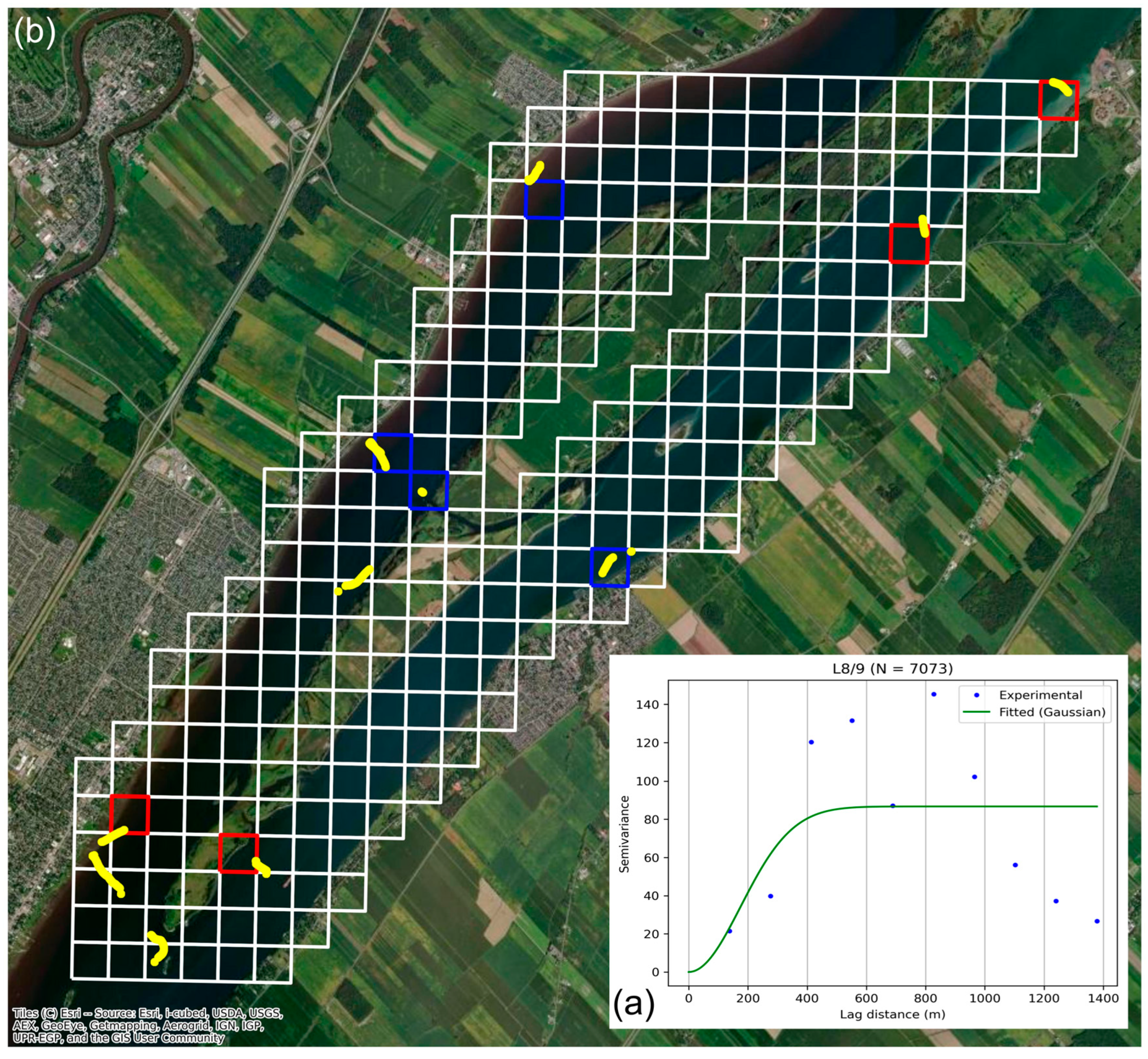
For model development, all spectral bands of L8/9 OLI, except the panchromatic band, and all spectral bands of Sentinel-2 MSI were used in this study. In addition to extracting per-pixel reflectance, mean and median kernels were computed using Window Sizes (WSs) of 3 × 3, 5 × 5, and 7 × 7 pixels. To reduce the impact of information leakage and spatial autocorrelation between training, validation, and test datasets, a spatial blocking approach [38] was adopted for data splitting. Specifically, a grid was superimposed over the study area, and random cells were progressively assigned to the test dataset until it contained at least 20% of the total samples. Using the same random selection process, another 20% of the samples were allocated to the validation dataset, while the remaining 60% were used for training. The cell size for spatial blocking was defined based on the semivariogram range of the in situ turbidity measurements, ensuring statistical independence between neighboring blocks. Semivariogram analyses were performed separately for the in situ turbidity measurements collected simultaneously with the S2 and L8/9 overpasses (Figure 2a and Figure 3a), revealing similar range values of ~400 m for both sensors. Consequently, a cell size of 400 m was adopted. Figure 2b and Figure 3b illustrate the spatial distribution of the in situ turbidity measurements corresponding to L8/9 and S2 acquisitions.

Figure 4 presents the ridge-density plots of the training, validation, and test datasets for both L8/9 and S2. Kernel density estimation was used to visualize the distribution of turbidity values for each dataset. To enable a clearer comparison among the three sets, all densities were normalized to a relative scale. The final training/validation/test ratios slightly deviated from the intended 60:20:20 split because the number of samples per grid cell varied, resulting in a 45.7:24.6:29.7 ratio for the S2 dataset due to a relatively dense final grid cell. This is an inevitable consequence of the spatial blocking approach.

The number of turbidity measurements with turbidity values exceeding 45 NTU was relatively limited compared to the number of turbidity measurements within the 0–40 NTU range (Figure 4); consequently, model training and performance evaluation are more reliable for turbidity values between 0 and 40 NTU, where data density is substantially higher than for turbidity values exceeding 45 NTU.

3.3. Regression Model

The LightGBM [39] model was used for turbidity estimation. LightGBM is a tree-based ensemble learning model that uses gradient boosting to iteratively minimize prediction errors. The model optimizes a loss function, which measures the difference between the estimated and measured turbidity values.

Model development and training procedures were implemented in Python version 3.10.17, using the LightGBM library version 4.6.0 [39]. To enhance model performance and prevent overfitting, key hyperparameters were optimized through the Optuna library version 4.3.0 [40], which applies a Bayesian optimization approach to explore the parameter space. The model was trained using the training dataset, while hyperparameter tuning was performed on the validation dataset to prevent overfitting. The tuning process aimed to minimize the RMSE using the validation dataset. After the model’s hyperparameters were finalized, the test dataset was used for final performance evaluation. The hyperparameters adjusted during tuning included the number of boosting iterations (n_estimators, varied from 1 to 200), the maximum tree depth (max_depth, between −1 and 200), the learning rate (learning_rate, between 0.0001 and 1), the fraction of features used per iteration (feature_fraction, between 0.0001 and 1.0), and the maximum number of leaves per tree (num_leaves, between 2 and 6). All other hyperparameters were retained at their default values. The optimization process was executed 200 times in Optuna. After running 200 trials in Optuna, the set of hyperparameters corresponding to the trial with the lowest RMSE on the validation dataset was selected for the final model.

Finally, regression models were trained and evaluated using each kernel (Section 3.2) for the three pre-processing options. For each pre-processing option, the kernel yielding the lowest RMSE for the test dataset was selected for comparison. After completing the evaluation phase, the entire dataset was used to train the final model, which was then applied to generate turbidity maps.

3.4. Performance Metrics

Three statistical metrics were employed as evaluation metrics: RMSE, ε [41], and β [41] (Equations (1)–(3)):

$$\mathrm{R}\mathrm{M}\mathrm{S}\mathrm{E}=\sqrt{{\displaystyle \frac{1}{\mathrm{N}}}{\sum }_{\mathrm{i}=1}^{\mathrm{N}}{\left({\mathrm{E}}_{\mathrm{i}}-{\mathrm{O}}_{\mathrm{i}}\right)}^2}$$

(1)

$$\mathsf{\beta }=100\times \mathrm{sign}\left[\mathrm{m}\mathrm{e}\mathrm{d}\mathrm{i}\mathrm{a}\mathrm{n}\left(\log {\displaystyle \frac{{\mathrm{E}}_{\mathrm{i}}}{{\mathrm{O}}_{\mathrm{i}}}}\right)\right]\times \left({\mathrm{e}}^{\left|\mathrm{m}\mathrm{e}\mathrm{d}\mathrm{i}\mathrm{a}\mathrm{n}\left(\log {\displaystyle \frac{{\mathrm{E}}_{\mathrm{i}}}{{\mathrm{O}}_{\mathrm{i}}}}\right)\right|}-1\right)$$

(2)

$$\mathsf{\epsilon }=100\times \left({\mathrm{e}}^{\mathrm{m}\mathrm{e}\mathrm{d}\mathrm{i}\mathrm{a}\mathrm{n}\left[\left|\log \left({\displaystyle \frac{{\mathrm{E}}_{\mathrm{i}}}{{\mathrm{O}}_{\mathrm{i}}}}\right)\right|\right]}-1\right)$$

(3)

$N$ is the number of observations, and $O$, $E$, $\overline{O}$, and $\overline{E}$ are the observations, estimated values, the average of the observations, and the average of the estimated values, respectively.

4. Results

4.1. Matchups

Figure 5 shows the RMSE values on the test dataset for L8/9 and S2, obtained from the LightGBM model trained using mean and median kernels with different WSs across the three pre-processing options. For L8/9, the median kernel with WS = 7 produced the lowest RMSE under the AE pre-processing option, WS = 5 under the AC pre-processing, and WS = 3 under the No pre-processing. For S2, the per-pixel reflectance (WS = 1) resulted in the lowest RMSE for both the No and AC pre-processing options, whereas the median kernel with WS = 7 achieved the best performance for the AE option.

As shown in Figure 5, the choice of kernel influenced RMSE. For example, under the AE pre-processing using the L8/9 dataset, replacing the median kernel (WS = 7) with a mean kernel (WS = 5) increased RMSE by ~156%.

4.2. Turbidity Retrieval

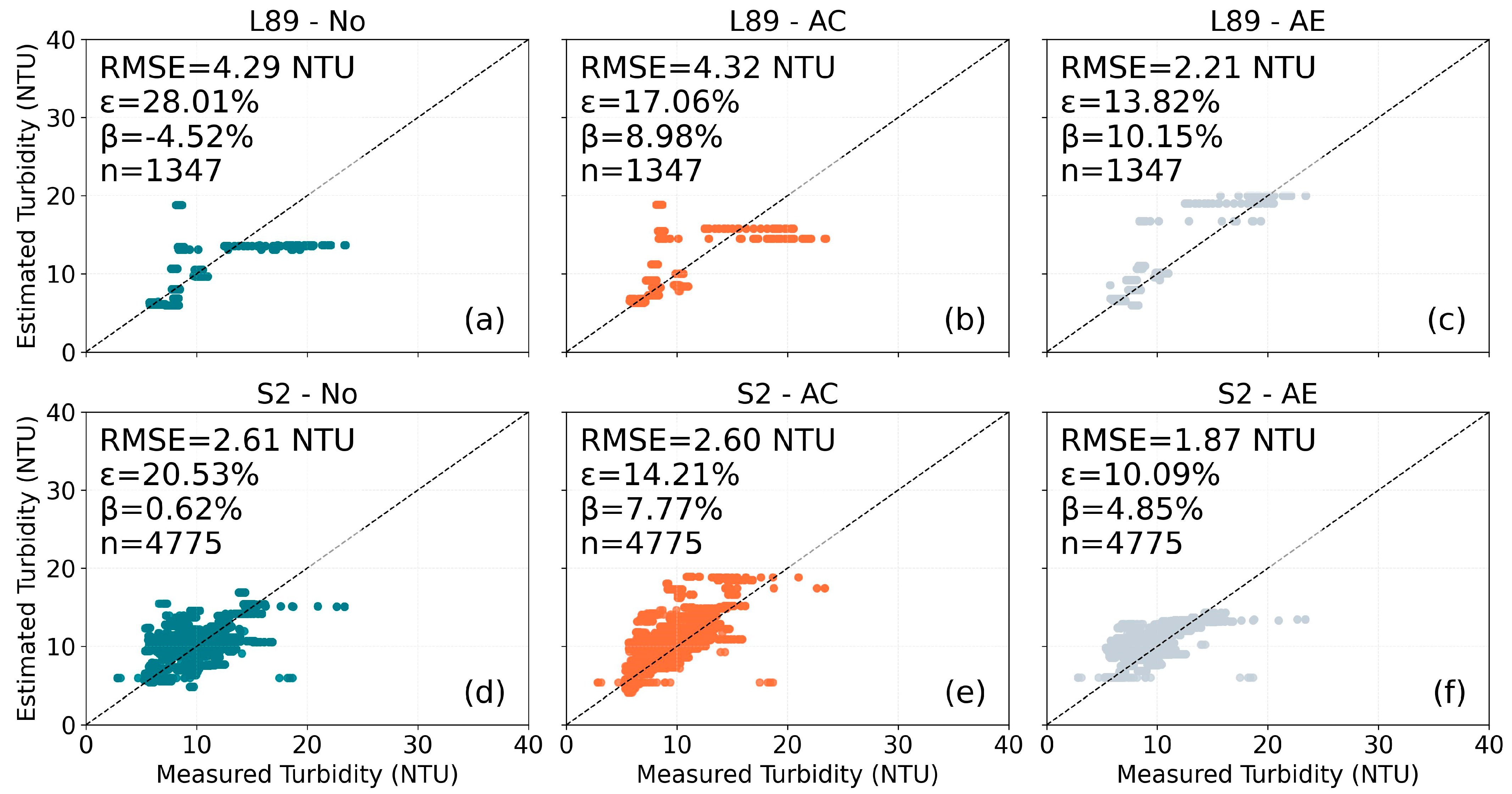
The tuned hyperparameters used for the LightGBM models are listed in

Table 2. Tuned hyperparameters of the LightGBM model for turbidity estimation under the three pre-processing options for both L8/9 and S2 datasets.

Sensor	Scenario	n_Estimators	Max_Depth	Learning_Rate	Feature_Fraction	Num_Leaves
L8/9	No	710	21	0.41	0.15	115
	AC	962	14	0.004	0.12	102
	AE	594	1	0.19	0.47	27
S2	No	223	0	0.22	0.22	20
	AC	259	49	0.10	0.75	5
	AE	362	37	0.05	0.22	2

. Figure 6 presents the scatterplots between the measured and estimated turbidity values using the test dataset. Each panel displays the RMSE, β, and ε metrics, calculated for the test dataset.

4.3. Variability of Correction Results with Distance to Shore

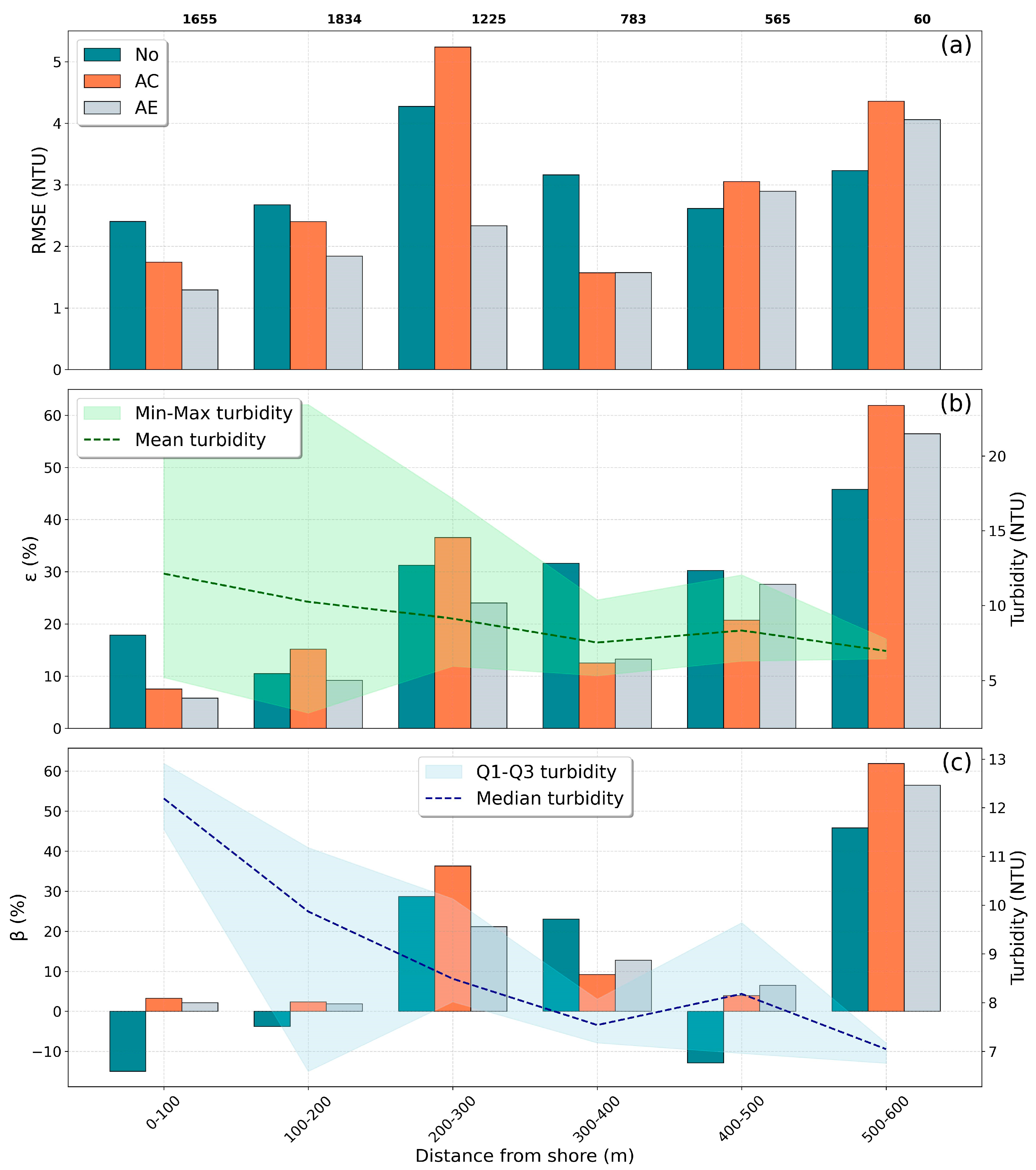
Figure 7 shows the variation in model performance with distance from the shore. As shown in Figure 7, the AE pre-processing exhibits superior performance compared to the other pre-processing options across all three metrics (RMSE, ε, and β) within 0–300 m from the shore.

4.4. Visual Comparison

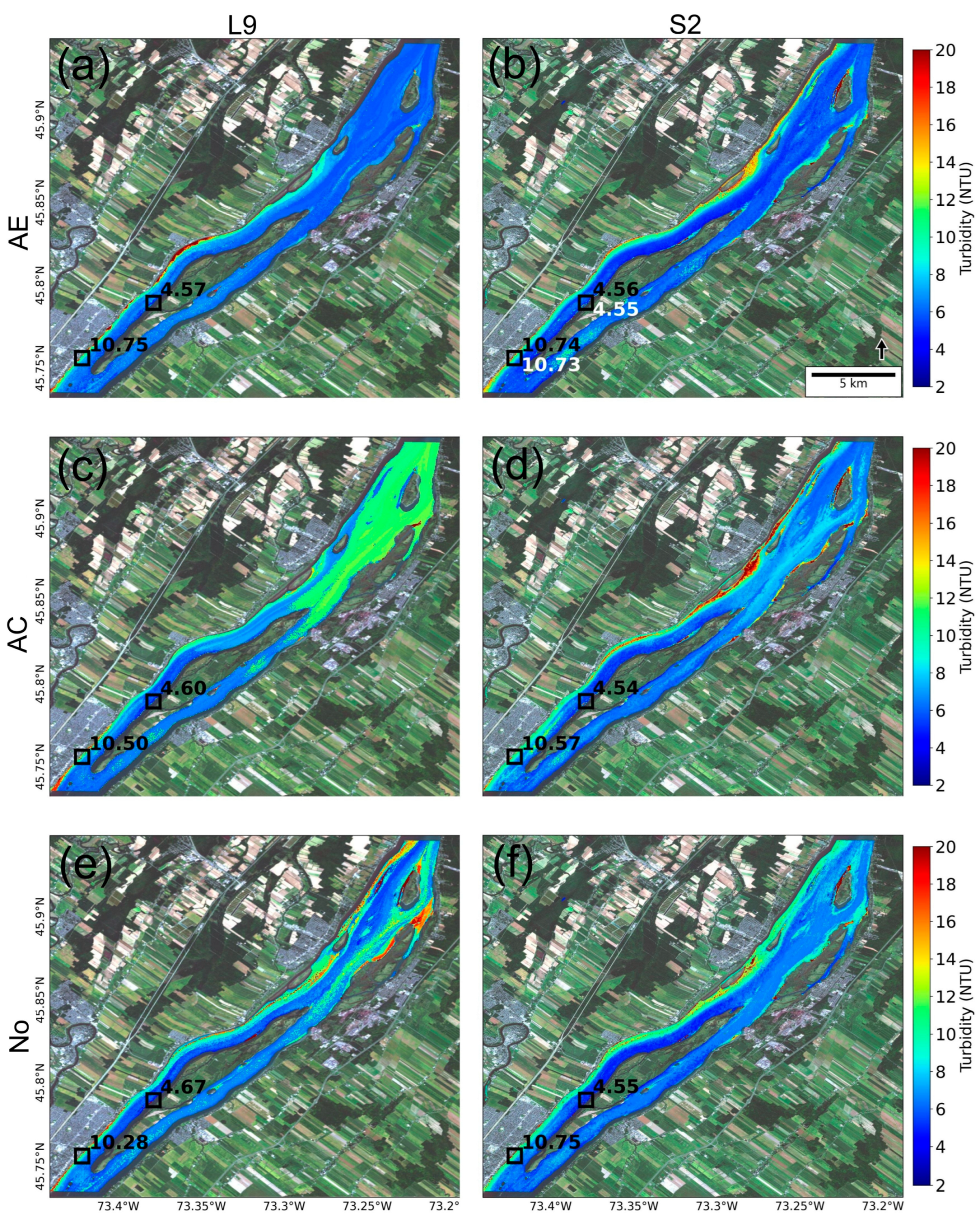
Figure 8 and Figure 9 present the turbidity maps generated using the three pre-processing options for 2 August 2024 and 11 September 2024, respectively. All maps show agreement with the field observations, capturing the overall spatial pattern of low turbidity along the southern shore (Site 1 in Figure 1a) and high turbidity along the northern shore (Site 2 in Figure 1a).

5. Discussion

5.1. Performance Comparison Among Pre-Processing Options

As shown in Figure 6a,b, for L8/9, applying DSF only (AC pre-processing) did not improve RMSE or |β| relative to TOA (No pre-processing): RMSE increased from 4.29 to 4.32 NTU, and |β| increased from 4.52% to 8.98%, corresponding to a 98.7% deterioration. However, the ε metric improved under the AC pre-processing, decreasing from 28.01% to 17.06%, which corresponds to a 39.1% reduction. Conversely, as illustrated in Figure 6b,c, introducing the AE correction with T-Mart improved performance, reducing RMSE from 4.32 to 2.21 NTU (an improvement of 48.8%) and ε from 17.06% to 13.82% (an improvement of 19.0%) compared to the AC pre-processing. Relative to the No pre-processing (Figure 6a,c), the AE pre-processing also enhanced performance: RMSE decreased by 48.5% and ε by 50.7%. Therefore, in terms of RMSE and ε, the AE pre-processing outperformed both the AC and the No pre-processing options. However, for |β|, the No pre-processing yielded the lowest value among all (β = −4.52%).

For S2, the AE pre-processing achieved the best performance in terms of RMSE and ε, followed by the AC pre-processing, while the No pre-processing exhibited the weakest performance. Specifically, RMSE and ε decreased from 2.61 NTU and 20.53% under the No pre-processing to 1.87 NTU and 10.09% under the AE pre-processing (Figure 6d,e), corresponding to improvements of approximately 28.4% and 50.8%, respectively. However, the No pre-processing yielded the lowest |β| compared to the other pre-processing options (β = 0.62%).

5.2. Variation in Scenario Performance with Shoreline Distance

As shown in Figure 7, within 0–300 m from the shoreline, where AE and turbidity levels are generally higher than those observed at 300–600 m based on mean and median values (Figure 7b,c), the AE pre-processing outperformed the other two pre-processing options. The superior performance of the AE option was most evident 200–300 m from shore, where RMSE decreased by >45% compared to the others.

From 0–300 m, RMSE increased with distance from the shoreline under all pre-processing options. However, the rate of increase was substantially lower for the AE pre-processing compared to the others. For instance, between 100 and 200 m and 200–300 m, RMSE increased by ~126% under the AC pre-processing but only by ~21% under the AE pre-processing. This indicates that model performance was more stable and consistent within 0–300 m when AE pre-processing was applied compared to when it was not.

Between 300 and 500 m, differences among the three pre-processing options become less clear, with performance varying across metrics rather than showing a single dominant approach. At distances greater than 500 m from the shoreline, the No pre-processing performed best across all metrics. However, the 500–600 m bin contained only 60 samples, which limits the strength of this conclusion. Overall, these results indicate that AE pre-processing is most important near the shoreline (0–300 m), performance becomes mixed in the middle range (300–500 m), and the No pre-processing performs best farther offshore (500–600 m).

5.3. Visual Assessment of Turbidity Maps

In Figure 8, a cloud is visible in the L8 image, which introduces noise in the turbidity maps generated by the AC and No pre-processing options (Figure 8c,e). The turbidity map derived from the AE pre-processing (Figure 8a) was less affected by this cloud, likely due to T-Mart treating clouds as reflecting surfaces and thus correcting for the AE from them in the processing. Additionally, in the lower-left part of the L8 turbidity maps, some artifacts were observed in the AC and No pre-processing options (Figure 8c,e), while the AE pre-processing remained cleaner and smoother in that region (Figure 8a).

The differences between the pre-processing options were more evident in the L9 maps shown in Figure 9. In the upper-right part of these maps, the AC and No pre-processing options (Figure 9c,e) exhibited noise, whereas the AE pre-processing (Figure 9a) produced a smoother spatial distribution. In the AC pre-processing (Figure 9c), the model appeared to fail in accurately predicting turbidity in the northeast section of the map. For S2, in Figure 8, the turbidity maps generated by the AE and AC pre-processing options (Figure 8b,d) were similar, and both performed better than the No pre-processing (Figure 8f), which showed some noise in the upper-right area. In contrast, Figure 9 clearly demonstrated that the AE pre-processing (Figure 9b) yielded a smoother and less noisy turbidity map compared to the other two pre-processing options.

6. Conclusions

This study compared three pre-processing options for turbidity estimation in the St. Lawrence River using S2 and L8/9 imagery with a LightGBM model: (1) the use of TOA reflectance data, (2) AC with DSF, and (3) AE correction using T-Mart followed by atmospheric correction with ACOLITE. The results demonstrated that the AE pre-processing improved RMSE and ε compared to the other two options, while the No pre-processing yielded the lowest |β|. Moreover, in terms of RMSE, the No and AC pre-processing options produced very similar values, whereas the AE pre-processing achieved improvements for both the S2 and L8/9 datasets. Additionally, the AE pre-processing produced smoother and more realistic turbidity maps compared to the other two pre-processing options, particularly in regions affected by cloud contamination. Performance patterns across shoreline distances further revealed that AE correction outperformed the alternatives within 0–300 m from the shore, where the AE is strong.

References

1. Ansari, M.; Knudby, A.; Amani, M.; Sawada, M. Retrieving Inland Water Quality Parameters via Satellite Remote Sensing: Sensor Evaluation, Atmospheric Correction, and Machine Learning Approaches. Remote Sens. 2025, 17, 1734. [Google Scholar] [CrossRef]
2. Cloern, J.E. Turbidity as a Control on Phytoplankton Biomass and Productivity in Estuaries. Cont. Shelf Res. 1987, 7, 1367–1381. [Google Scholar] [CrossRef]
3. Liu, W.; Wang, S.; Yang, R.; Ma, Y.; Shen, M.; You, Y.; Hai, K.; Baqa, M.F. Remote Sensing Retrieval of Turbidity in Alpine Rivers Based on High Spatial Resolution Satellites. Remote Sens. 2019, 11, 3010. [Google Scholar] [CrossRef]
4. Mishra, D.R.; Ogashawara, I.; Gitelson, A.A. Bio-Optical Modeling and Remote Sensing of Inland Waters; Elsevier: Amsterdam, The Netherlands, 2017; ISBN 978-0-12-804654-8. [Google Scholar]
5. IOCCG. Atmospheric Correction for Remotely-Sensed Ocean-Colour Products; IOCCG Report Series; International Ocean Colour Coordinating Group: Dartmouth, NS, Canada, 2010. [Google Scholar]
6. Hu, C.; Carder, K.L.; Muller-Karger, F.E. Atmospheric Correction of SeaWiFS Imagery over Turbid Coastal Waters: A Practical Method. Remote Sens. Environ. 2000, 74, 195–206. [Google Scholar] [CrossRef]
7. Ruddick, K.G.; Ovidio, F.; Rijkeboer, M. Atmospheric Correction of SeaWiFS Imagery for Turbid Coastal and Inland Waters. Appl. Opt. 2000, 39, 897–912. [Google Scholar] [CrossRef]
8. Tanré, D.; Deschamps, P.Y.; Duhaut, P.; Herman, M. Adjacency Effect Produced by the Atmospheric Scattering in Thematic Mapper Data. J. Geophys. Res. Atmos. 1987, 92, 12000–12006. [Google Scholar] [CrossRef]
9. Pahlevan, N.; Mangin, A.; Balasubramanian, S.V.; Smith, B.; Alikas, K.; Arai, K.; Barbosa, C.; Bélanger, S.; Binding, C.; Bresciani, M.; et al. ACIX-Aqua: A Global Assessment of Atmospheric Correction Methods for Landsat-8 and Sentinel-2 over Lakes, Rivers, and Coastal Waters. Remote Sens. Environ. 2021, 258, 112366. [Google Scholar] [CrossRef]
10. Vanhellemont, Q.; Ruddick, K. Atmospheric Correction of Metre-Scale Optical Satellite Data for Inland and Coastal Water Applications. Remote Sens. Environ. 2018, 216, 586–597. [Google Scholar] [CrossRef]
11. Vanhellemont, Q. Adaptation of the Dark Spectrum Fitting Atmospheric Correction for Aquatic Applications of the Landsat and Sentinel-2 Archives. Remote Sens. Environ. 2019, 225, 175–192. [Google Scholar] [CrossRef]
12. Ouma, Y.O. Modelling Reservoir Turbidity from Medium Resolution Sentinel-2A/MSI and Landsat-8/OLI Satellite Imagery. In Proceedings of the Remote Sensing for Agriculture, Ecosystems, and Hydrology XXII, SPIE, Bellingham, WA, USA, 20 September 2020; Volume 11528, pp. 111–117. [Google Scholar] [CrossRef]
13. Wang, Q.; Liu, G.; Song, K.; Wen, Z.; Shang, Y.; Li, S.; Fang, C.; Tao, H. Comparison of Machine Learning Algorithms for Estimating Global Lake Clarity With Landsat TOA Data. IEEE Trans. Geosci. Remote Sens. 2024, 62, 4206514. [Google Scholar] [CrossRef]
14. Ge, Y.; Shen, F.; Sklenička, P.; Vymazal, J.; Baxa, M.; Chen, Z. Machine Learning for Cyanobacteria Inversion via Remote Sensing and AlgaeTorch in the Třeboň Fishponds, Czech Republic. Sci. Total Environ. 2024, 947, 174504. [Google Scholar] [CrossRef] [PubMed]
15. Begliomini, F.N.; Barbosa, C.C.F.; Martins, V.S.; Novo, E.M.L.M.; Paulino, R.S.; Maciel, D.A.; Lima, T.M.A.; O’Shea, R.E.; Pahlevan, N.; Lamparelli, M.C. Machine Learning for Cyanobacteria Mapping on Tropical Urban Reservoirs Using PRISMA Hyperspectral Data. ISPRS J. Photogramm. Remote Sens. 2023, 204, 378–396. [Google Scholar] [CrossRef]
16. Hieronymi, M.; Krasemann, H.; Mueller, D.; Brockmann, C.; Ruescas, A.; Stelzer, K.; Nechad, B.; Ruddick, K.; Simis, S.; Tilstone, G.; et al. Ocean Colour Remote Sensing of Extreme Case-2 Waters. Proc. ESA Living Planet Symp. 2016, SP-740, Sco 3-1. [Google Scholar]
17. Wu, Y.; Knudby, A.; Lapen, D. Topography-adjusted Monte Carlo simulation of the adjacency effect in remote sensing of coastal and inland waters. J. Quant. Spectrosc. Radiat. Transf. 2023, 303, 108589. [Google Scholar] [CrossRef]
18. Castagna, A.; Vanhellemont, Q. A Generalised Physics-Based Correction for Adjacency Effects. Appl. Opt. 2025, 64, 2719–2743. [Google Scholar] [CrossRef]
19. Pan, Y.; Bélanger, S. Genetic Algorithm for Atmospheric Correction (GAAC) of Water Bodies Impacted by Adjacency Effects. Remote Sens. Environ. 2025, 317, 114508. [Google Scholar] [CrossRef]
20. Wu, Y.; Knudby, A.; Pahlevan, N.; Lapen, D.; Zeng, C. Sensor-Generic Adjacency-Effect Correction for Remote Sensing of Coastal and Inland Waters. Remote Sens. Environ. 2024, 315, 114433. [Google Scholar] [CrossRef]
21. Kwon, S.; Noh, H.; Seo, I.W.; Park, Y.S. Effects of Spectral Variability Due to Sediment and Bottom Characteristics on Remote Sensing for Suspended Sediment in Shallow Rivers. Sci. Total Environ. 2023, 878, 163125. [Google Scholar] [CrossRef]
22. Wu, Z.; Pang, J.; Li, J.; Wang, Y.; Ruan, J.; Zhang, X.; Yang, L.; Pang, Y.; Gao, Y. A Review of Remote Sensing-Based Water Quality Monitoring in Turbid Coastal Waters. Intell. Mar. Technol. Syst. 2025, 3, 24. [Google Scholar] [CrossRef]
23. Ansari, M.; Knudby, A.; Homayouni, S. River Salinity Mapping through Machine Learning and Statistical Modeling Using Landsat 8 OLI Imagery. Adv. Space Res. 2025, 75, 6981–7002. [Google Scholar] [CrossRef]
24. Khan, R.M.; Salehi, B.; Niroumand-Jadidi, M.; Mahdianpari, M. Mapping Water Clarity in Small Oligotrophic Lakes Using Sentinel-2 Imagery and Machine Learning Methods: A Case Study of Canandaigua Lake in Finger Lakes, New York. IEEE J. Sel. Top. Appl. Earth Obs. Remote Sens. 2024, 17, 4674–4688. [Google Scholar] [CrossRef]
25. Mamun, M.; Hasan, M.; An, K.-G. Advancing Reservoirs Water Quality Parameters Estimation Using Sentinel-2 and Landsat-8 Satellite Data with Machine Learning Approaches. Ecol. Inform. 2024, 81, 102608. [Google Scholar] [CrossRef]
26. Zhou, Y.; Li, W.; Cao, X.; He, B.; Feng, Q.; Yang, F.; Liu, H.; Kutser, T.; Xu, M.; Xiao, F.; et al. Spatial-Temporal Distribution of Labeled Set Bias Remote Sensing Estimation: An Implication for Supervised Machine Learning in Water Quality Monitoring. Int. J. Appl. Earth Obs. Geoinf 2024, 131, 103959. [Google Scholar] [CrossRef]
27. Adjovu, G.E.; Stephen, H.; James, D.; Ahmad, S. Measurement of Total Dissolved Solids and Total Suspended Solids in Water Systems: A Review of the Issues, Conventional, and Remote Sensing Techniques. Remote Sens. 2023, 15, 3534. [Google Scholar] [CrossRef]
28. Adjovu, G.E.; Stephen, H.; Ahmad, S. A Machine Learning Approach for the Estimation of Total Dissolved Solids Concentration in Lake Mead Using Electrical Conductivity and Temperature. Water 2023, 15, 2439. [Google Scholar] [CrossRef]
29. Richardson, G.; Knudby, A.; Wu, Y.; Ansari, M. A Case Study Comparing Approaches to Mask Satellite-Derived Bathymetry. Discov. Geosci. 2025, 3, 103. [Google Scholar] [CrossRef]
30. Ansari, M.; Akhoondzadeh, M. Mapping Water Salinity Using Landsat-8 OLI Satellite Images (Case Study: Karun Basin Located in Iran). Adv. Space Res. 2020, 65, 1490–1502. [Google Scholar] [CrossRef]
31. Ansari, M.; Akhoondzadeh, M. Generation of Karun River Water Salinity Map from Landsat-8 Satellite Images using Support Vector Regression, Multilayer Perceptron and Genetic Algorithm. J. Environ. Stud. 2021, 46, 581–600. [Google Scholar] [CrossRef]
32. Vachon, D. Water Quality in the Fluvial Section Physicochemical and Bacteriological Parameters, 5th ed.; Canada Water Agency: Winnipeg, MB, Canada, 2023; ISBN 978-0-660-77291-2. [Google Scholar]
33. EcoLogic LLC, St. Lawrence River Watershed Characterization Report; Franklin County Soil & Water Conservation District: Louisburg, NC, USA, 2019.
34. Merriman, J. Water Quality in the St. Lawrence River at Wolfe Island; Environment Canada: Gatineau, QC, Canada, 1997; ISBN 978978-1-100-17523-2. [Google Scholar]
35. Global Modeling and Assimilation Office (GMAO). MERRA-2 tavg1_2d_aer_Nx: 2d,1-Hourly,Time-Averaged,Single-Level,Assimilation,Aerosol Diagnostics, V5.12.4; Goddard Earth Sciences Data and Information Services Center (GES DISC): Greenbelt, MD, USA, 2015. [Google Scholar] [CrossRef]
36. Harmel, T.; Chami, M.; Tormos, T.; Reynaud, N.; Danis, P.-A. Sunglint Correction of the Multi-Spectral Instrument (MSI)-SENTINEL-2 Imagery over Inland and Sea Waters from SWIR Bands. Remote Sens. Environ. 2018, 204, 308–321. [Google Scholar] [CrossRef]
37. OBPG. Ancillary Data. Available online: https://oceancolor.gsfc.nasa.gov/resources/docs/ancillary/ (accessed on 5 September 2025).
38. Knudby, A.; Richardson, G. Incorporation of Neighborhood Information Improves Performance of SDB Models. Remote Sens. Appl. Soc. Environ. 2023, 32, 101033. [Google Scholar] [CrossRef]
39. Ke, G.; Meng, Q.; Finley, T.; Wang, T.; Chen, W.; Ma, W.; Ye, Q.; Liu, T.-Y. LightGBM: A Highly Efficient Gradient Boosting Decision Tree. In Proceedings of the Advances in Neural Information Processing Systems, Long Beach, CA, USA, 4–9 December 2017; Curran Associates, Inc.: Red Hook, NY, USA, 2017; Volume 30. [Google Scholar]
40. Akiba, T.; Sano, S.; Yanase, T.; Ohta, T.; Koyama, M. Optuna: A Next-Generation Hyperparameter Optimization Framework. In Proceedings of the 25th ACM SIGKDD International Conference on Knowledge Discovery & Data Mining, New York, NY, USA, 25 July 2019; Association for Computing Machinery: New York, NY, USA, 2019; pp. 2623–2631. [Google Scholar]
41. Morley, S.K.; Brito, T.V.; Welling, D.T. Measures of Model Performance Based On the Log Accuracy Ratio. Space Weather 2018, 16, 69–88. [Google Scholar] [CrossRef]
Figure 1. Study area: the St. Lawrence River, Montréal, QC, Canada. (a) Sampling locations where turbidity measurements were collected during four field campaigns; each campaign is shown in a different color. (b) Location of the case study area. (c) Map showing turbidity values at each measurement location. (d) Example water samples collected at Sites 1 and 2 (in panel (a)) on 7 August 2024.
Remotesensing 18 00127 g001
Figure 2. Spatial distribution of in situ turbidity measurements corresponding to L8/9 acquisitions (a) and their experimental semivariogram (b). Yellow points indicate the locations of in situ turbidity measurements, while the overlaid grid represents the spatial blocking scheme used for data splitting. Cells outlined in red denote the test dataset, those outlined in blue represent the validation dataset, and the remaining cells were assigned for model training.
Remotesensing 18 00127 g002
Figure 3. Spatial distribution of in situ turbidity measurements corresponding to S2 acquisitions (a) and their experimental semivariogram (b). Yellow points indicate the locations of in situ turbidity measurements, while the overlaid grid represents the spatial blocking scheme used for data splitting. Cells outlined in red denote the test dataset, those outlined in blue represent the validation dataset, and the remaining cells were assigned for model training.
Remotesensing 18 00127 g003
Figure 4. Ridge-density plots of in situ turbidity measurements in the training, validation, and test datasets for (a) L8/9 and (b) S2 matchups. Kernel density estimates are shown for values up to 45 NTU, with densities encoded using a continuous color scale. Samples exceeding 45 NTU are represented as aggregated bars. Summary statistics and sample counts for each dataset are provided within each subplot.
Remotesensing 18 00127 g004
Figure 5. RMSE values on the test dataset for (a) L8/9 and (b) S2, obtained from the LightGBM model trained using per-pixel and kernel-based (mean and median with 3 × 3, 5 × 5, and 7 × 7 window sizes) reflectance inputs across the three pre-processing options. The star symbol marks the kernel that achieved the lowest RMSE for each pre-processing option.
Remotesensing 18 00127 g005
Figure 6. Scatterplots comparing measured and estimated turbidity values obtained from the LightGBM model for L8/9 (top row; panels (ac)) and S2 (bottom row; panels (df)). Each column corresponds to one pre-processing option: No (first column; panels (a,d)), AC (second column; panels (b,e)), and AE (third column; panels (c,f)). Text shows RMSE, β, ε, and the number of samples for the test dataset.
Remotesensing 18 00127 g006
Figure 7. Variability of model performance metrics with distance to the shore, combining test data from L8/9 and S2 sensors. (a) Changes in RMSE with distance to the shore, where the numbers above the bars indicate the number of samples within each distance interval. (b) ε (left y-axis) alongside the minimum, maximum, and mean turbidity values (right y-axis) represented by the green shaded polygon. (c) β (left y-axis) with the interquartile range and median turbidity (right y-axis) illustrated by the blue shaded polygon.
Remotesensing 18 00127 g007
Figure 8. Spatial distribution of turbidity estimates on 2 August 2024, derived from L8/9 (left column; panels (a,c,e)) and S2 (right column; panels (b,d,f)). Each row represents a different pre-processing option: AE (top row; panels (a,b)), AC (middle row; panels (c,d)), and No (bottom row; panels (e,f)). Black labels indicate estimated turbidity values, while white labels on the upper-right map (panel (b)) show in situ turbidity measurements. The north arrow and scale bar are shown in the lower-right corner of panel (b) and are common to all panels.
Remotesensing 18 00127 g008
Figure 9. Spatial distribution of turbidity estimates on 11 September 2024, derived from L8/9 (left column; panels (a,c,e)) and S2 (right column; panels (b,d,f)). Each row represents a different pre-processing option: AE (top row; panels (a,b)), AC (middle row; panels (c,d)), and No (bottom row; panels (e,f)). Black labels indicate estimated turbidity values, while white labels on the upper-right map (panel (b)) show in situ turbidity measurements. The north arrow and scale bar are shown in the lower-right corner of panel (b) and are common to all panels.
Remotesensing 18 00127 g009